
Optimization of Water Pressure of a Distribution Network within the Water–Energy Nexus

 ,
,  ,
,  and
and
Abstract
1. Introduction
2. Materials and Methods
2.1. WDN Simulation
2.2. Water Leakage Simulation
2.3. Burst Frequency Simulation
2.4. Energy Consumption Simulation for Domestic Water Pressure Booster Systems
2.5. Optimization Method
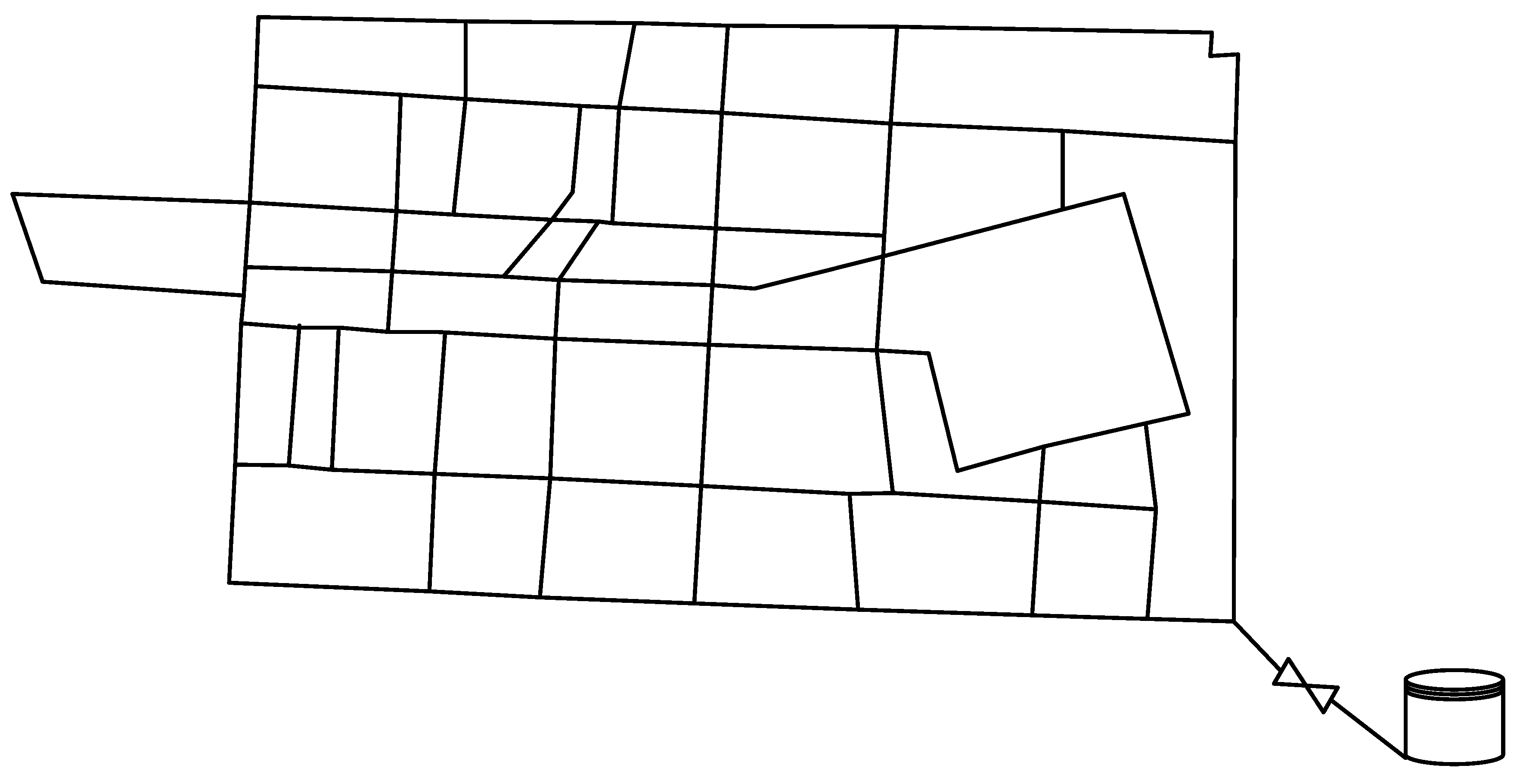
3. Case Study
- Preparation of hydraulic parameters of the existing water network (information of nodes and network pipes).
- Implementing genetic algorithm for determining the parameters with uncertainty.
- Conducting the optimization process for calibration by calculating the mean absolute percentage error (MAPE) using Equation (11).
- 4.
- Comparing the empirical and calculated results at each iteration.
- 5.
- Calculating the objective function and finally obtaining the optimal solution in which the defined conditions for calibration is satisfied.
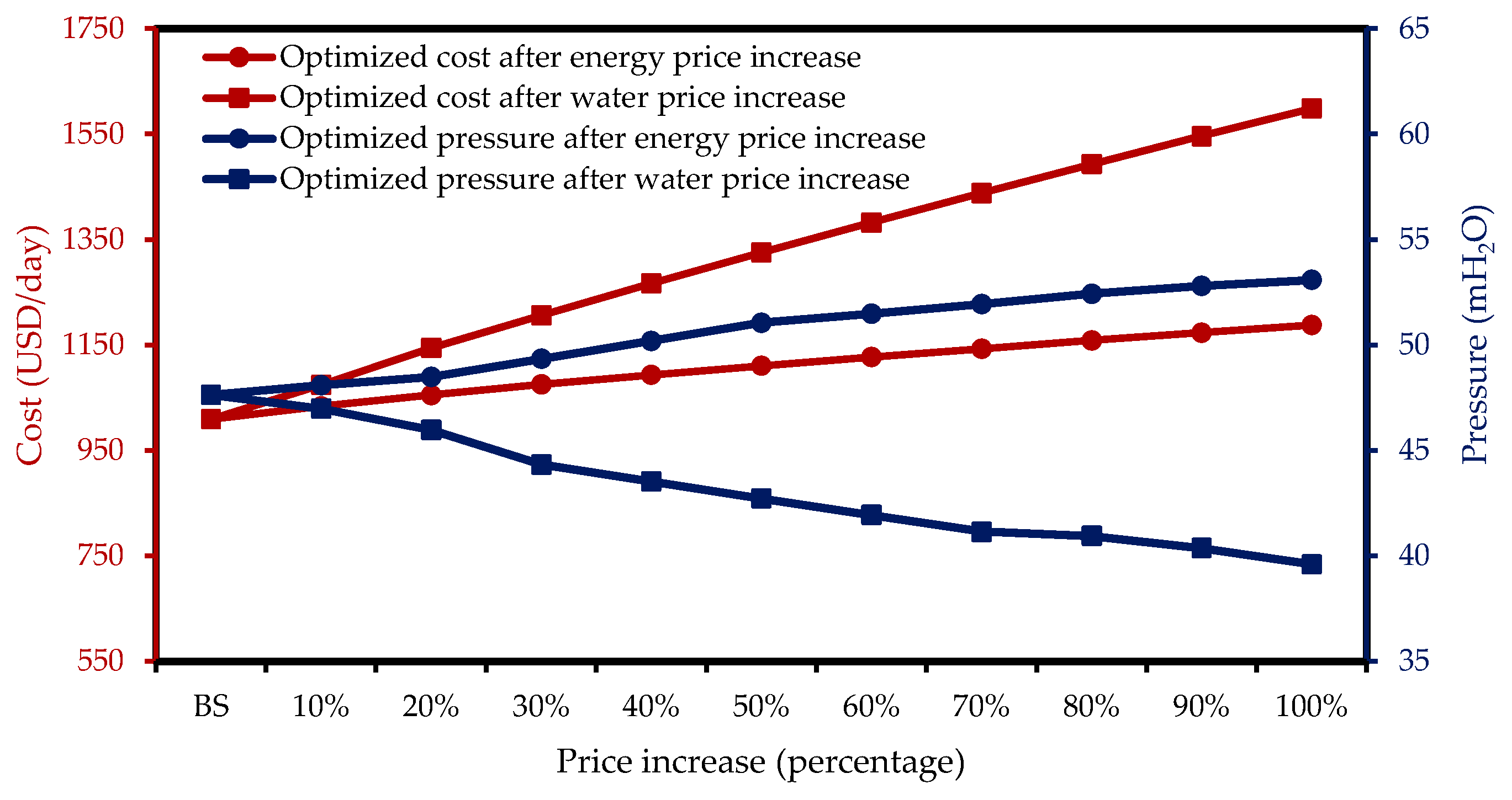
4. Results and Discussion
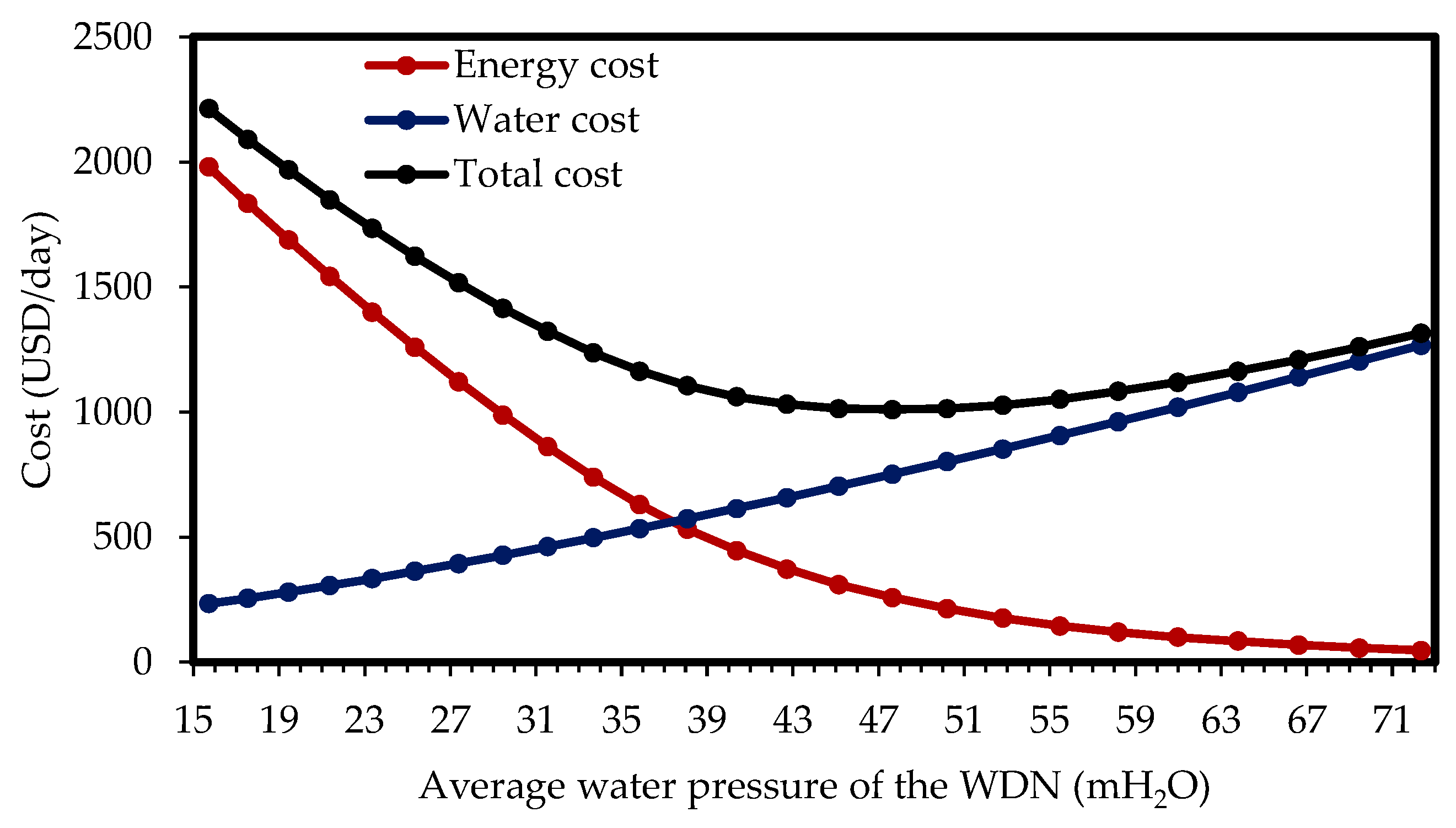
4.1. Daily Pressure Optimization
4.2. Hourly-Based Pressure Optimization
5. Conclusions
- Without an integrated approach to the water and energy sectors, choosing an optimized pressure for any WDN can be misleading.
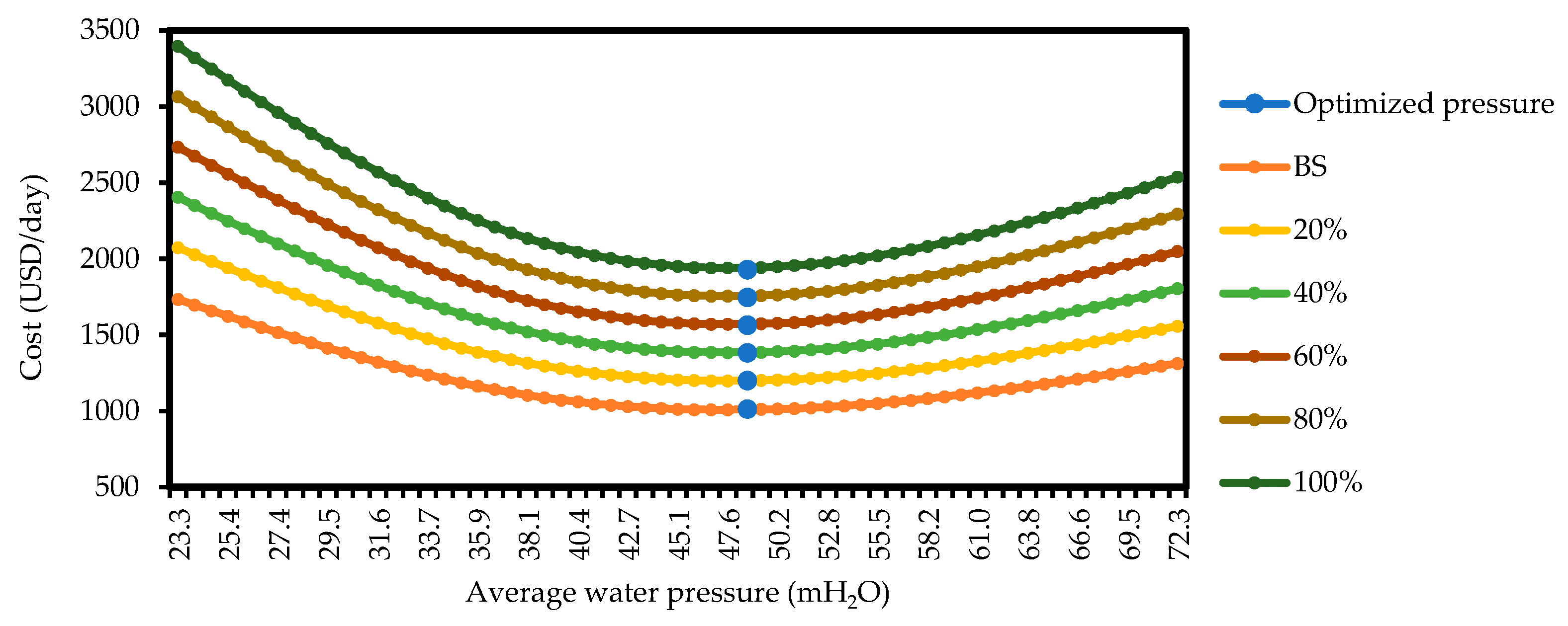
- The optimal water network pressure based on daily measurements for the case study was found to be 47.6 mH2O (total daily cost = USD 1009). The sensitivity analysis on the input variables showed that the optimized cost and optimized pressure are most sensitive to the leakage exponent and physical water loss, respectively.
- The optimal pressure can be calculated either daily or hourly. Because of the sensitivity of the model to the hourly water consumption pattern and energy prices, the average optimal pressure varied from one hour to the next. When the optimal pressure of the network was calculated based on hourly measurements, the total daily cost was reduced by about 41% (USD 598).
Author Contributions
Funding
Institutional Review Board Statement
Informed Consent Statement
Data Availability Statement
Acknowledgments
Conflicts of Interest
Nomenclature
| Symbols | |
| BF | Burst frequency |
| c | Price (USD) |
| C | Cost (USD) |
| g | Acceleration of the gravity (9.8 m s−2) |
| h | Pumping head (mH2O) |
| H | Pressure head (mH2O) |
| L | Leakage (m3) |
| n | Head exponent |
| m | Number of data for calibration |
| N1 | Leakage exponent |
| N2 | Burst exponent |
| P | Power (Kwh) |
| q | Required water flow (l s−1) |
| Q | Water discharge (l s−1) |
Abbreviations
| DDSM | Demand driven simulation method |
| HDSM | Head driven simulation system |
| FAVAD | Fixed and variable area discharges |
| RTC | Real time control |
| PRV | Pressure reducing valve |
| WPBS | Water pressure booster system |
| WDN | Water distribution network |
| Greek symbols | |
| η | Efficiency |
| Density (kg m−3) | |
| Subscripts and superscripts | |
| ave | Average |
| avl | Available |
| b | Head dependent portion |
| B | Break |
| des | Design |
| E | Energy |
| elv | Elevation |
| j | Node |
| loss | Friction loss |
| min | Minimum |
| max | Maximum |
| npd | Non-pressure dependent |
| req | Required |
| sup | Supplied |
| W | Water |
References
- Nasrollahi, H.; Ahmadi, F.; Ebadollahi, M.; Najafi Nobar, S.; Amidpour, M. The greenhouse technology in different climate conditions: A comprehensive energy-saving analysis. Sustain. Energy Technol. Assess. 2021, 47, 101455. [Google Scholar] [CrossRef]
- Andric, I.; Kamal, A.; Al-Ghamdi, S.G. Efficiency of green roofs and green walls as climate change mitigation measures in extremely hot and dry climate: Case study of Qatar. Energy Rep. 2020, 6, 2476–2489. [Google Scholar] [CrossRef]
- Nafil, A.; Bouzi, M.; Anoune, K.; Ettalabi, N. Comparative study of forecasting methods for energy demand in Morocco. Energy Rep. 2020, 6, 523–536. [Google Scholar] [CrossRef]
- Nasrollahi, H.; Shirazizadeh, R.; Shirmohammadi, R.; Pourali, O.; Amidpour, M. Unraveling the Water-Energy-Food-Environment Nexus for Climate Change Adaptation in Iran: Urmia Lake Basin Case-Study. Water 2021, 13, 1282. [Google Scholar] [CrossRef]
- Petrakopoulou, F.; Robinson, A.; Olmeda-Delgado, M. Impact of climate change on fossil fuel power-plant efficiency and water use. J. Clean. Prod. 2020, 273, 122816. [Google Scholar] [CrossRef]
- Jung, D.; Kim, J.H. Water Distribution System Design to Minimize Costs and Maximize Topological and Hydraulic Reliability. J. Water Resour. Plan. Manag. 2018, 144, 06018005. [Google Scholar] [CrossRef]
- Fan, X.Y.; Klemeš, J.J.; Jia, X.; Liu, Z.Y. An iterative method for design of total water networks with multiple contaminants. J. Clean. Prod. 2019, 240, 118098. [Google Scholar] [CrossRef]
- Meirelles Lima, G.; Brentan, B.M.; Luvizotto, E. Optimal design of water supply networks using an energy recovery approach. Renew. Energy 2018, 117, 404–413. [Google Scholar] [CrossRef]
- Marques, J.; Cunha, M.; Savić, D. Many-objective optimization model for the flexible design of water distribution networks. J. Environ. Manag. 2018, 226, 308–319. [Google Scholar] [CrossRef] [PubMed]
- Monsef, H.; Naghashzadegan, M.; Jamali, A.; Farmani, R. Comparison of evolutionary multi objective optimization algorithms in optimum design of water distribution network. Ain Shams Eng. J. 2019, 10, 103–111. [Google Scholar] [CrossRef]
- Zhang, Y.; Li, S.; Zheng, Y.; Zou, Y. Multi-model based pressure optimization for large-scale water distribution networks. Control Eng. Pract. 2020, 95, 104232. [Google Scholar] [CrossRef]
- Lambert, A. What Do We Know About Pressure:Leakage Relationships In Distribution Systems? In Proceedings of the IWA Conference on Systems Approach to Leakage Control and Water Distribution System Management, Brno, Czech Republic, 16–18 May 2001. [Google Scholar]
- Ghorbanian, V.; Guo, Y.; Karney, B. Field Data–Based Methodology for Estimating the Expected Pipe Break Rates of Water Distribution Systems. J. Water Resour. Plan. Manag. 2016, 142, 4016040. [Google Scholar] [CrossRef]
- Chang, D.E.; Yoo, D.G.; Kim, J.H. Practical head-outflow relationship definition methodology that accounts for varied water-supply methods. Sustainability 2020, 12, 4755. [Google Scholar] [CrossRef]
- Chang, D.E.; Yoo, D.G.; Kim, J.H. A study on the practical pressure-driven hydraulic analysis method considering actual water supply characteristics of water distribution network. Sustainability 2021, 13, 2793. [Google Scholar] [CrossRef]
- Fabbiano, L.; Vacca, G.; Dinardo, G. Smart water grid: A smart methodology to detect leaks in water distribution networks. Measurement 2020, 151, 107260. [Google Scholar] [CrossRef]
- Puust, R.; Kapelan, Z.; Savic, D.A.; Koppel, T. A review of methods for leakage management in pipe networks. Urban Water J. 2010, 7, 25–45. [Google Scholar] [CrossRef]
- Nicolini, M.; Zovatto, L. Optimal location and control of pressure reducing valves in water networks. J. Water Resour. Plan. Manag. 2009, 135, 178–187. [Google Scholar] [CrossRef]
- Vicente, D.J.; Garrote, L.; Sánchez, R.; Santillán, D. Pressure Management in Water Distribution Systems: Current Status, Proposals, and Future Trends. J. Water Resour. Plan. Manag. 2016, 142, 04015061. [Google Scholar] [CrossRef]
- Ferrarese, G.; Malavasi, S. Perspectives of water distribution networks with the greenvalve system. Water 2020, 12, 1579. [Google Scholar] [CrossRef]
- Rajakumar, A.G.; Cornelio, A.A.; Mohan Kumar, M.S. Leak management in district metered areas with internal-pressure reducing valves. Urban Water J. 2020, 17, 714–722. [Google Scholar] [CrossRef]
- Mosetlhe, T.C.; Hamam, Y.; Du, S.; Monacelli, E. A survey of pressure control approaches in water supply systems. Water 2020, 12, 1732. [Google Scholar] [CrossRef]
- Campisano, A.; Modica, C.; Reitano, S.; Ugarelli, R.; Bagherian, S. Field-Oriented Methodology for Real-Time Pressure Control to Reduce Leakage in Water Distribution Networks. J. Water Resour. Plan. Manag. 2016, 142, 04016057. [Google Scholar] [CrossRef]
- Araujo, L.S.; Ramos, H.; Coelho, S.T. Pressure control for leakage minimisation in water distribution systems management. Water Resour. Manag. 2006, 20, 133–149. [Google Scholar] [CrossRef]
- Thornton, J.; Lambert, A. Progress in practical prediction of pressure: Leakage, pressure: Burst frequency and pressure: Consumption relationships. In Proceedings of the IWA Special Conferences’ Leakage, Halifax, NS, Canada, 12–14 September 2005; pp. 12–14. [Google Scholar]
- Kanakoudis, V.K.; Tolikas, D.K. The role of leaks and breaks in water networks: Technical and economical solutions. J. Water Supply Res. Technol. 2001, 50, 301–311. [Google Scholar] [CrossRef]
- Mann, E.; Frey, J. Optimized pipe renewal programs ensure cost-effective asset management. In Pipelines 2011: A Sound Conduit for Sharing Solutions; Proc. Pipelines 2011 Conf.; American Society of Civil Engineers: Reston, VA, USA, 2011; pp. 44–54. [Google Scholar] [CrossRef]
- Creaco, E.; Walski, T. Economic Analysis of Pressure Control for Leakage and Pipe Burst Reduction. J. Water Resour. Plan. Manag. 2017, 143, 04017074. [Google Scholar] [CrossRef]
- Filion, Y.R.; MacLean, H.L.; Karney, B.W. Life-Cycle Energy Analysis of a Water Distribution System. J. Infrastruct. Syst. 2004, 10, 120–130. [Google Scholar] [CrossRef]
- Menke, R.; Kadehjian, K.; Abraham, E.; Stoianov, I. Investigating trade-offs between the operating cost and green house gas emissions from water distribution systems. Sustain. Energy Technol. Assess. 2017, 21, 13–22. [Google Scholar] [CrossRef]
- Cabrera, E.; Cobacho, R.; Soriano, J. Towards an energy labelling of pressurized water networks. Procedia Eng. 2014, 70, 209–217. [Google Scholar] [CrossRef]
- Sharif, M.N.; Haider, H.; Farahat, A.; Hewage, K.; Sadiq, R. Water–energy nexus for water distribution systems: A literature review. Environ. Rev. 2019, 27, 519–544. [Google Scholar] [CrossRef]
- Menke, R.; Abraham, E.; Parpas, P.; Stoianov, I. Demonstrating demand response from water distribution system through pump scheduling. Appl. Energy 2016, 170, 377–387. [Google Scholar] [CrossRef]
- Hashemi, S.S.; Tabesh, M.; Ataeekia, B. Ant-colony optimization of pumping schedule to minimize the energy cost using variable-speed pumps in water distribution networks. Urban Water J. 2014, 11, 335–347. [Google Scholar] [CrossRef]
- Giustolisi, O.; Berardi, L.; Laucelli, D. Supporting decision on energy vs. asset cost optimization in drinking water distribution networks. Procedia Eng. 2014, 70, 734–743. [Google Scholar] [CrossRef][Green Version]
- Abdallah, M.; Kapelan, Z. Fast Pump Scheduling Method for Optimum Energy Cost and Water Quality in Water Distribution Networks with Fixed and Variable Speed Pumps. J. Water Resour. Plan. Manag. 2019, 145, 04019055. [Google Scholar] [CrossRef]
- Colombo, A.F.; Karney, B.W. Energy and costs of leaky pipes: Toward comprehensive picture. J. Water Resour. Plan. Manag. 2002, 128, 441–450. [Google Scholar] [CrossRef]
- Shao, Y.; Yu, Y.; Yu, T.; Chu, S.; Liu, X. Leakage Control and Energy Consumption Optimization in the Water Distribution Network Based on Joint Scheduling of Pumps and Valves. Energies 2019, 12, 2969. [Google Scholar] [CrossRef]
- Todini, E.; Pilati, S. A gradient algorithm for the analysis of pipe networks. In Computer Applications in Water Supply: Vol. 1—Systems Analysis and Simulation; John Wiley & Sons: London, UK, 1988; pp. 1–20. [Google Scholar]
- Tabesh, M.; Doulatkhah, A. Effects of pressure dependent analysis on quality performance assessment of water distribution networks. Iran. J. Sci. Technol. Trans. 2006, 30, 119–128. [Google Scholar]
- Gupta, R.; Bhave, P.R. Comparison of Methods for Predicting Deficient-Network Performance. J. Water Resour. Plan. Manag. 1996, 122, 214–217. [Google Scholar] [CrossRef]
- Tabesh, M. Implications of the Pressure Dependency of Outflows of Data Management, Mathematical Modelling and Reliability Assessment of Water Distribution Systems; University of Liverpool: Liverpool, UK, 1998. [Google Scholar]
- Wu, Z.Y.; Wang, R.H.; Walski, T.M.; Yang, S.Y.; Bowdler, D.; Baggett, C.C. Extended Global-Gradient Algorithm for Pressure-Dependent Water Distribution Analysis. J. Water Resour. Plan. Manag. 2009, 135, 13–22. [Google Scholar] [CrossRef]
- Tabesh, M.; Shirzad, A.; Arefkhani, V.; Mani, A. A comparative study between the modified and available demand driven based models for head driven analysis of water distribution networks. Urban Water J. 2014, 11, 221–230. [Google Scholar] [CrossRef]
- Shirzad, A.; Tabesh, M. Study of pressure-discharge relations in water distribution networks using field measurements. In Proceedings of the IWA World Water Congress and Exhibition, Busan, Korea, 16–21 September 2012; Volume 8328. [Google Scholar]
- Gorev, N.B.; Kodzhespirova, I.F. Noniterative Implementation of Pressure-Dependent Demands Using the Hydraulic Analysis Engine of EPANET 2. Water Resour. Manag. 2013, 27, 3623–3630. [Google Scholar] [CrossRef]
- Rasekh, A.; Brumbelow, K. Drinking water distribution systems contamination management to reduce public health impacts and system service interruptions. Environ. Model. Softw. 2014, 51, 12–25. [Google Scholar] [CrossRef]
- Abdy Sayyed, M.A.H.; Gupta, R.; Tanyimboh, T.T. Noniterative Application of EPANET for Pressure Dependent Modelling Of Water Distribution Systems. Water Resour. Manag. 2015, 29, 3227–3242. [Google Scholar] [CrossRef][Green Version]
- Awad, H.; Kapelan, Z.; Savić, D. Analysis of pressure management economics in water distribution systems. In Proceedings of the 10th Annual Water Distribution Systems Analysis Conference WDSA 2008; American Society of Civil Engineers: Reston, VA, USA, 2009; pp. 520–531. [Google Scholar] [CrossRef]
- Sousa, J.; Martinho, N.; Muranho, J.; Marques, A.S. Leakage Calibration in Water Distribution Networks with Pressure-Driven Analysis: A Real Case Study. Environ. Sci. Proc. 2020, 2, 59. [Google Scholar] [CrossRef]
- Berardi, L.; Giustolisi, O. Calibration of Design Models for Leakage Management of Water Distribution Networks. Water Resour. Manag. 2021, 35, 2537–2551. [Google Scholar] [CrossRef]
- Fantozzi, M.; Lambert, A. Including the effects of pressure management in calculations of Short-Run Economic Leakage Levels. In Proceedings of the IWA Conference “Water Loss 2007”, Bucharest, Romania, 23–26 September 2007. [Google Scholar]
- Deyi, M.; van Zyl, J.; Shepherd, M. Applying the FAVAD Concept and Leakage Number to Real Networks: A Case Study in Kwadabeka, South Africa. Procedia Eng. 2014, 89, 1537–1544. [Google Scholar] [CrossRef]
- Van Zyl, J.E.; Clayton, C.R.I. The effect of pressure on leakage in water distribution systems. In Proceedings of the Institution of Civil Engineers—Water Management; Thomas Telford Ltd.: London, UK, 2007; Volume 160, pp. 109–114. [Google Scholar]
- Lambert, A.; Fantozzi, M.; Thornton, J. Practical approaches to modeling leakage and pressure management in distribution systems–progress since 2005. In Proceedings of the 12th International Conference on Computing and Control for the Water Industry—CCWI2013, London, UK, 2–4 September 2013. [Google Scholar]
- Diaz, C.; Ruiz, F.; Patino, D. Modeling and control of water booster pressure systems as flexible loads for demand response. Appl. Energy 2017, 204, 106–116. [Google Scholar] [CrossRef]
- Grundfos. GRUNDFOS Water Pressure Boosting. Domest. Build. Serv. 2017, 1, 1–12. [Google Scholar]
- Emiliawati, A. A study of water pump efficiency for household water demand at Lubuklinggau. In Proceedings of the AIP Conference Proceedings; AIP Publishing LLC: Melville, NY, USA, 2017; Volume 1903, p. 100003. [Google Scholar]
- Shankar, V.K.A.; Umashankar, S.; Paramasivam, S.; Hanigovszki, N. A comprehensive review on energy efficiency enhancement initiatives in centrifugal pumping system. Appl. Energy 2016, 181, 495–513. [Google Scholar] [CrossRef]
- Olszewski, P. Genetic optimization and experimental verification of complex parallel pumping station with centrifugal pumps. Appl. Energy 2016, 178, 527–539. [Google Scholar] [CrossRef]
- Augustyn, T. Energy efficiency and savings in pumping systems—The holistic approach. In Proceedings of the 2012 Southern African Energy Efficiency Convention (SAEEC), Johannesburg, South Africa, 14–15 November 2012; IEEE: Piscataway Township, NJ, USA, 2012; pp. 1–7. [Google Scholar]
- Tabesha, M.; Jamasbb, M.; Moeini, R. Calibration of water distribution hydraulic models: A comparison between pressure dependent and demand driven analyses. Urban Water J. 2011, 8, 93–102. [Google Scholar] [CrossRef]
- Supervision, I.R. of I.V.P. for S.P. and Guidelines for Design of Urban and Rural Water Supply and Destribuion Systems. 2013. Available online: http://waterstandard.wrm.ir/cs/WRMResearch/278/220 (accessed on 23 July 2021). (In Persian).
- Statistical Center of Iran. The Report of Population General Census in Iran; Statistical Center of Iran: Tehran, Iran, 2019. (In Persian) [Google Scholar]


| Node | Elevation (m) | Base Demand (L/s) | Node | Elevation (m) | Base Demand (L/s) | Node | Elevation (m) | Base Demand (L/s) |
|---|---|---|---|---|---|---|---|---|
| 1 | 1592 | 8 | 25 | 1551 | 8 | 49 | 1565 | 4 |
| 2 | 1575 | 3 | 26 | 1556 | 16 | 50 | 1571 | 2 |
| 3 | 1583 | 8 | 27 | 1566 | 15 | 51 | 1573 | 2 |
| 4 | 1572 | 7 | 28 | 1570 | 6 | 52 | 1585 | 4 |
| 5 | 1585 | 1 | 29 | 1569 | 8 | 53 | 1586 | 2 |
| 6 | 1585 | 8 | 30 | 1566 | 13 | 54 | 1556 | 4 |
| 7 | 1592 | 7 | 31 | 1563 | 10 | 55 | 1555 | 4 |
| 8 | 1588 | 7 | 32 | 1566 | 5 | 56 | 1559 | 4 |
| 9 | 1588 | 7 | 33 | 1565 | 5 | 57 | 1559 | 3 |
| 10 | 1584 | 5 | 34 | 1562 | 9 | 58 | 1571 | 4 |
| 11 | 1569 | 7 | 35 | 1554 | 10 | 59 | 1573 | 1 |
| 12 | 1568 | 12 | 36 | 1596 | 4 | 60 | 1576 | 4 |
| 13 | 1562 | 12 | 37 | 1598 | 4 | 61 | 1557 | 1 |
| 14 | 1553 | 13 | 38 | 1561 | 3 | 62 | 1586 | 5 |
| 15 | 1590 | 2 | 39 | 1563 | 4 | 63 | 1586 | 4 |
| 16 | 1559 | 3 | 40 | 1589 | 4 | 64 | 1567 | 4 |
| 17 | 1552 | 7 | 41 | 1586 | 1 | 65 | 1567 | 5 |
| 18 | 1550 | 4 | 42 | 1574 | 9 | 66 | 1556 | 2 |
| 19 | 1552 | 7 | 43 | 1572 | 9 | 67 | 1554 | 1 |
| 20 | 1566 | 4 | 44 | 1563 | 3 | 68 | 1561 | 6 |
| 21 | 1584 | 8 | 45 | 1563 | 10 | 69 | 1561 | 2 |
| 22 | 1554 | 8 | 46 | 1568 | 5 | 70 | 1579 | 2 |
| 23 | 1551 | 12 | 47 | 1569 | 2 | 71 | 1579 | 4 |
| 24 | 1565 | 5 | 48 | 1563 | 5 |
| Pipe | Length (m) | Diameter (mm) | Pipe | Length (m) | Diameter (mm) | Pipe | Length (m) | Diameter (mm) |
|---|---|---|---|---|---|---|---|---|
| 1 | 675 | 180 | 37 | 407 | 140 | 73 | 132 | 280 |
| 2 | 657 | 500 | 38 | 400 | 180 | 74 | 130 | 140 |
| 3 | 657 | 280 | 39 | 393 | 100 | 75 | 113 | 450 |
| 4 | 657 | 500 | 40 | 390 | 450 | 76 | 111 | 140 |
| 5 | 638 | 250 | 41 | 387 | 100 | 77 | 91 | 125 |
| 6 | 620 | 250 | 42 | 380 | 100 | 78 | 85 | 560 |
| 7 | 618 | 100 | 43 | 379 | 355 | 79 | 60 | 630 |
| 8 | 618 | 450 | 44 | 363 | 140 | 80 | 1 | 225 |
| 9 | 544 | 355 | 45 | 353 | 315 | 81 | 604 | 560 |
| 10 | 539 | 280 | 46 | 349 | 450 | 82 | 1324 | 500 |
| 11 | 534 | 250 | 47 | 321 | 630 | 83 | 1023 | 400 |
| 12 | 528 | 280 | 48 | 316 | 280 | 84 | 875 | 180 |
| 13 | 524 | 100 | 49 | 305 | 125 | 85 | 846 | 500 |
| 14 | 519 | 280 | 50 | 275 | 100 | 86 | 829 | 500 |
| 15 | 515 | 100 | 51 | 274 | 125 | 87 | 781 | 500 |
| 16 | 515 | 125 | 52 | 269 | 225 | 88 | 729 | 630 |
| 17 | 514 | 450 | 53 | 262 | 100 | 89 | 727 | 280 |
| 18 | 513 | 355 | 54 | 262 | 100 | 90 | 727 | 225 |
| 19 | 512 | 225 | 55 | 262 | 500 | 91 | 726 | 500 |
| 20 | 511 | 140 | 56 | 257 | 100 | 92 | 718 | 500 |
| 21 | 510 | 450 | 57 | 250 | 315 | 93 | 714 | 100 |
| 22 | 508 | 100 | 58 | 248 | 560 | 94 | 709 | 280 |
| 23 | 508 | 280 | 59 | 243 | 160 | 95 | 706 | 100 |
| 24 | 505 | 500 | 60 | 239 | 125 | 96 | 698 | 355 |
| 25 | 500 | 100 | 61 | 223 | 100 | 97 | 693 | 280 |
| 26 | 498 | 315 | 62 | 219 | 280 | 98 | 1010 | 140 |
| 27 | 496 | 400 | 63 | 216 | 125 | 99 | 2156 | 160 |
| 28 | 492 | 315 | 64 | 209 | 125 | 100 | 422 | 180 |
| 29 | 479 | 100 | 65 | 205 | 100 | 101 | 704 | 225 |
| 30 | 470 | 560 | 66 | 199 | 630 | 102 | 629 | 160 |
| 31 | 464 | 450 | 67 | 195 | 225 | 103 | 633 | 140 |
| 32 | 438 | 180 | 68 | 191 | 500 | 104 | 625 | 125 |
| 33 | 438 | 630 | 69 | 185 | 125 | 105 | 619 | 100 |
| 34 | 435 | 100 | 70 | 177 | 200 | 106 | 620 | 180 |
| 35 | 432 | 500 | 71 | 161 | 100 | 107 | 622 | 280 |
| 36 | 429 | 140 | 72 | 143 | 125 |
| Value | Unit | |
|---|---|---|
| Input data for EPANET | ||
| Total base demand | 407 | L/s |
| Total pipes length | 511 | km |
| Material of pipes | Polyethylene | - |
| Hazen–Williams coefficient | 130 | - |
| Input data for calculating Qjavl in HDSM | ||
| Hjmin | 0 | mH2O |
| Hjdes | 30 | mH2O |
| Hjmax | 100 | mH2O |
| n | 2.08 | - |
| Input data for calculating leakage cost | ||
| L0 (have,0 = 45 m) | 0.2 × Qjavl | L/s |
| N1 | 1.4 | - |
| cw | 0.05 | $/m3 |
| Input data for calculating burst cost | ||
| BF0 (have,0 = 45 m) | 4 | Number/day |
| BFnpd | 1 | Number/day |
| N2 | 3 | - |
| cB | 80 | $/burst |
| Input data for optimization function | ||
| Hmin | 10 | mH2O |
| Hmax | 100 | mH2O |
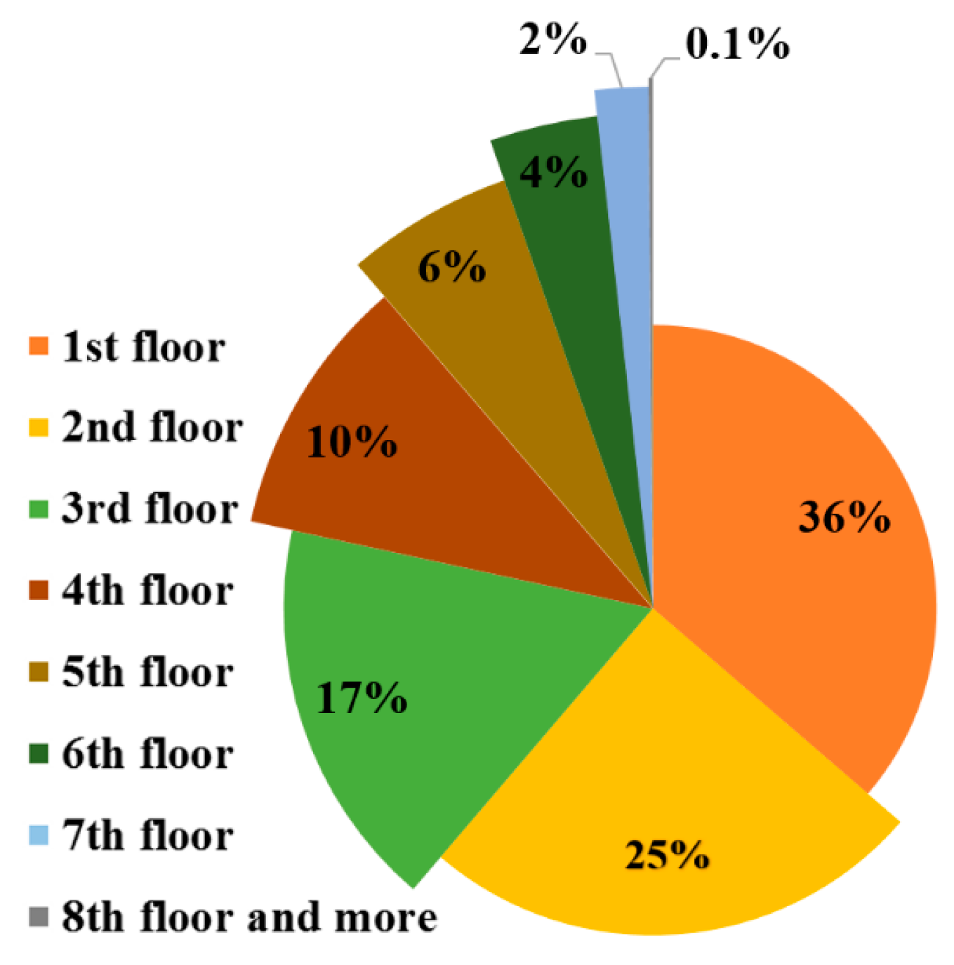
| Value | Unit | |
|---|---|---|
| Input data for calculating power consumed by WPBS | ||
| Population | 79,023 | - |
| Housing census | 25,118 | - |
| Number of buildings | 11,081 | - |
| floor to floor height of buildings | 3.2 | m |
| η | 20 | % |
| Input data for calculating the energy cost | ||
| cE | 0.0064 (23 p.m.–8 a.m.) | $/KWh |
| 0.0080 (8 a.m.–16 p.m.) | $/KWh | |
| 0.1040 (16 p.m.–23 p.m.) | $/KWh | |
Publisher’s Note: MDPI stays neutral with regard to jurisdictional claims in published maps and institutional affiliations. |
© 2021 by the authors. Licensee MDPI, Basel, Switzerland. This article is an open access article distributed under the terms and conditions of the Creative Commons Attribution (CC BY) license (https://creativecommons.org/licenses/by/4.0/).
Share and Cite
Nasrollahi, H.; Safaei Boroujeni, R.; Shirmohammadi, R.; Najafi Nobar, S.; Aslani, A.; Amidpour, M.; Petrakopoulou, F. Optimization of Water Pressure of a Distribution Network within the Water–Energy Nexus. Appl. Sci. 2021, 11, 8371. https://doi.org/10.3390/app11188371
Nasrollahi H, Safaei Boroujeni R, Shirmohammadi R, Najafi Nobar S, Aslani A, Amidpour M, Petrakopoulou F. Optimization of Water Pressure of a Distribution Network within the Water–Energy Nexus. Applied Sciences. 2021; 11(18):8371. https://doi.org/10.3390/app11188371
Chicago/Turabian StyleNasrollahi, Hossein, Reza Safaei Boroujeni, Reza Shirmohammadi, Shima Najafi Nobar, Alireza Aslani, Majid Amidpour, and Fontina Petrakopoulou. 2021. "Optimization of Water Pressure of a Distribution Network within the Water–Energy Nexus" Applied Sciences 11, no. 18: 8371. https://doi.org/10.3390/app11188371
APA StyleNasrollahi, H., Safaei Boroujeni, R., Shirmohammadi, R., Najafi Nobar, S., Aslani, A., Amidpour, M., & Petrakopoulou, F. (2021). Optimization of Water Pressure of a Distribution Network within the Water–Energy Nexus. Applied Sciences, 11(18), 8371. https://doi.org/10.3390/app11188371