Optimized Sensors Network and Dynamical Maps for Monitoring Traffic Noise in a Large Urban Zone

Abstract

We review a Dynamap European Life project whose main scope was the design, commissioning, and actual implementation of “real-time” acoustic maps in a district of the city of Milan (District 9, or Z9, composed of about 2000 road stretches), by employing a small number of noise monitoring stations within the urban zone. Dynamap is based on the idea of finding suitable sets of roads displaying similar daily traffic noise behavior, so that one can group them together into single dynamical noise maps. The Dynamap sensor network has been built upon twenty-four monitoring stations, which have been permanently installed in appropriate locations within the pilot zone Z9, by associating four sensors to each one of the six group of roads considered. In order to decide which road stretches belong to a group, a non-acoustic parameter is used, which is obtained from a traffic flow model of the city, developed and tested over the years by the “Enviroment, Mobility and Territory Agency” of Milan (EMTA). The fundamental predictive equation of Dynamap, for the local equivalent noise level at a given site, can be built by using real-time data provided by the monitoring sensors. In addition, the corresponding contributions of six static traffic noise maps, associated with the six group of roads, are required. The static noise maps can be calculated from the Cadna noise model, based on EMTA road traffic data referred to the ‘rush-hour’ (8:00–9:00 a.m.), when the road traffic flow is maximum and the model most accurate. A further analysis of road traffic noise measurements, performed over the whole city of Milan, has provided a more accurate description of road traffic noise behavior by using a clustering approach. It is found that essentially just two mean cluster hourly noise profiles are sufficient to represent the noise profile at any site location within the zone. In order words, one can use the 24 monitoring stations data to estimate the local noise variations at a single site in real time. The different steps in the construction of the network are described in detail, and several validation tests are presented in support of the Dynamap performance, leading to an overall error of about 3 dB. The present work ends with a discussion of how to improve the design of the network further, based on the calculation of the cross-correlations between monitoring stations’ noise data.

1. Introduction

Noise mapping is becoming a necessary tool for evaluating the noise exposure of citizens in large cities, as it has been recognized by the strict dose–harmful effect relationships reported both in the European Directive 2002/49/EC (Environmental Noise Directive, END) [1] and the 2018 WHO Environmental noise guidelines [2]. Strategic noise maps have been implemented to enable effective diagnostics of the acoustic environment, providing useful information for local intervention measures and policy-making decisions [3]. They evaluate the overall exposure to noise in a given area due to different sources and, together with Action Plans, provide a framework to manage environmental noise and its effects. Thus, they represent the standard approach for noise prevention and control. The deployment of distributed acoustic monitoring stations in urban and suburban areas started about a decade ago, in concomitance with the lowering costs of electronic components and the availability of efficient hardware for data transfer. Such extended monitoring technique has continuously grown in popularity since the publication of the END by the recognition that acoustic maps represent a powerful tool for determining the exposure of population to environmental noise.

Until recently, noise maps were normally obtained by using mean vehicle flows, averaged over a period of one year, but this simple approach clearly lacks accuracy when dealing with varying noise on a daily basis. As a result, noise maps had been evolving towards a multi-source predictive approach [4,5,6,7,8]. It then became clear that instead ‘dynamical’ (i.e., time dependent) noise maps should be developed for obtaining realistic and accurate noise predictions over shorter time scales. In other words, the introduction of dynamic noise maps constitutes a further evolution in the direction of better representing the actual noise exposure.

The Dynamap project, dubbed ‘Dynamic Acoustic Mapping: Development of low cost sensors networks for real-time noise mapping’ [9,10,11,12], is a LIFE project (ref. LIFE13 ENV/IT/001254), aimed at developing a dynamic noise mapping system, enabling to detect and represent the acoustic impact of road infrastructures in real time. Since the update of noise maps using a standard approach requires the collection and processing of a huge amount of data, such a procedure would be very time consuming and costly, having a significant impact on the financial statements of the authorities responsible for providing noise maps. Therefore, more elaborated solutions are required in order to reduce the cost of noise mapping activities.

To meet such requirements, and the growing demand of information about noise pollution, the Dynamap project foresees the development of an automated noise mapping system delivering real-time (short-term) noise maps, as well as long-term noise assessments. Despite real-time noise maps not being explicitly required by END (see Appendix A), their automated generation is estimated to lower the cost of noise mapping conspicuously (see DYNAMAP—Development of low cost sensor networks for real time noise mapping, LIFE Projects 2013, Environment Policy, and Governace—July 2014: Publications [12]), with added significant benefits for noise managers and receivers. As a result, the Dynamap system is expected to lead to a significant reduction in the resources needed to update the noise maps (time, costs, and dedicated personnel), and to improve and facilitate the dissemination of information to the public through appropriate web tools and/or the opportunity to abate noise with alternative measures based on traffic control and management. The system is aimed at providing easy and handy information, which can be complemented with additional information regarding multiple environmental data dynamically, such as air quality, meteorological conditions, etc. [12].

The paper is organized as follows. In Section 2, we present a brief review of the state of the art on noise mapping relevant to Dynamap. Section 3 is devoted to the Dynamap approach, describing the theory and its fundamental equations: The Dynamap traffic noise sensors network is discussed in Section 3.1, the group traffic noise variations of each dynamical map are defined in Section 3.2 and Section 3.3, the implementation, location of the Dynamap sensor network, and its operation are reported. The results are presented in Section 4, including additional measurement sites to assess the group components in Section 4.1, the validation of Dynamap in Section 4.2, the correlations between sensor locations and how to optimize the network in Section 4.3, and the correlations of Dynamap predictions with measurements in Section 4.4. Finally, Section 5 is devoted to the Conclusions.

2. State of the Art

In Section 2.1, we present a brief summary of the state of the art on road traffic noise mapping, referring to some of the relevant works to our review published within the last two decades. In Section 2.2, we discuss the generalities of the Dynamap system with a particular emphasis on its innovative characteristics, and in Section 2.3, the spatial and temporal structure of road traffic noise in large urban zones.

2.1. Related Works Relevant to the Dynamap Project

The classification of streets plays an important role for Dynamap. Different attempts are known, and we refer to a few of them. A street categorization has been developed for the city of Valladolid (Spain) [13], and an urban noise functional stratification has been studied for estimating average annual sound level [14]. Closely related to this issue is the problem of identifying the type of vehicle producing the noise, e.g., vehicle sound signature recognition by frequency vector principal component analysis [15], a dimensionality reduction approach for detection of moving vehicles [16], techniques of acoustic feature extraction for detection and classification of ground vehicles [17], noise source identification with Beamforming in the pass-by of a car [18], a scaling model for a speed-dependent vehicle noise spectrum [19], and a vehicle speed recognition from noise spectral patterns [20].

Health related issues due to traffic and environmental noise has attracted a great deal of attention over the years. Annoyance issues due to the transportation and their relationships with exposure metrics have been studied [21]. A study of some effects of aircraft noise on cognitive performance in schoolchildren has been reported [22], as well as the relation between ambient noise and cognitive processes among primary schoolchildren [23]. Noise and mental performance quantified by personality attributes and noise sensitivity have been considered [24], in addition to the important issue of traffic noise and risk of myocardial infarction [25]. Of prime importance is also the relation between environmental noise, sleep, and health, as discussed in [26]. Long-term road traffic noise exposure is also associated with an increase in morning tiredness [27]; in addition, transportation noise resulted in increased blood pressure in adults [28]. Further work includes the exposure modifiers of the relationships of transportation noise with high blood pressure and noise annoyance [29], the quantitative relationship between road traffic noise and hypertension from the point of view of meta-analysis [30]. A recent, updated study on health-related issues of noise has been published by the WHO [2].

From a larger geographical perspective, there is interest in the environmental burden of disease in Europe by assessing risk factors in some countries [31], also yielding an international scale implementation of the CNOSSOS-EU road traffic noise prediction model for epidemiological studies [32]. This can be extended to a global noise score indicator for classroom evaluation of acoustic performances in the LIFE GIOCONDA project, allowing a comparison between different classrooms or schools, based on their acoustic performances, and a homogeneous evaluation of the priority for planning noise mitigation actions in Italian schools [33]. Research has been performed to suggest a selection of suitable alternatives to reduce the environmental impact of road traffic noise using a fuzzy multi-criteria decision model [34]. Annoyance evaluation has been performed due to overall railway noise and vibration in Pisa (Italy) urban areas, showing the limitations of traditional noise mapping for railway epidemiological studies based exclusively on ordinary transits, thus confirming the role of vibrations as enhancing factor for disturbance [35]. A laboratory study has been reported on noise annoyance assessment of various urban road vehicle pass-by noises in isolation and combined with industrial noise [36]. A survey on exposure–response relationships for road, rail, and aircraft noise annoyance, and the differences between continuous and intermittent noise have been considered [37]. The application of the intermittency ratio (IR) metric for the classification of urban sites based on road traffic noise events has been studied and proved to be a useful supplementary metric to the equivalent level, which measures only the energy content of the noise exposure [38]. Finally, a classification of urban road traffic noise based on sound energy and eventfulness indicators, such as the IR, have been considered recently by taking into account measured sound fluctuations in a large urban zone [39].

The important issue of the assessment of transportation noise due to railways, airports, and high-noise plants have been discussed extensively. Examples include an assessment of railway noise in an urban setting, pointing to the problems the nearby living population experiences due to the railway noise pollution [40], the ADS-B (Automatic Dependent Surveillance-Broadcast) system, which has proved to be a useful tool for testing and redrawing noise management strategies at Pisa airport, producing cost-effective solutions for the airport noise management in urban areas, particularly when the radar tracks are not available [41], and a novel method to determine multiexposure priority indices tested for the Pisa action plan has been developed, called Multi Annoyance Building Prioritisation Score (MABPS), which takes into account the annoyance due to the exposure from different sources (multiexposure), showing significant differences with standard methods [42]. Of related interest is the transportation planning for quiet natural areas preservation based on aircraft overflights’ noise assessment in a National Park [43]. This is connected to the more technical issue of wind turbine noise, for which a technical procedure has been suggested to simultaneously estimate the emmission and the residual noise components measured nearby a wind farm when the residual noise is mainly generated by wind, thus allowing the evaluation of the noise impact produced by operational wind farms, without requiring the farm shut down [44]. In addition, the exposure to wind turbine noise has been evaluated by means of perceptual responses and reported health effects [45]. In addition, a metric reflecting short-term temporal variations of transportation noise exposure has been discussed [46]. As a way to restore some mitigation to the environment, the so-called green wall has been studied as a sustainable tool in Mediterranean cities, such as of Limassol (Cyprus) [47]. A case study in Malaysia residential streets has been reported [48], while the impact of the ring road conclusion to the city of Guimaraes (Portugal) has been analyzed from the point of view of traffic flow variations and accessibilities [49].

Noise mapping has a long history, and we report some related recent works. In [50], the authors consider a context sensitive noise impact mapping, while, in [51], the spatial sampling for night levels estimation in urban environments is studied. The development of a practical framework for strategic noise mapping is considered in [52], while, in [4], a noise mapping in the EU is studied using models and procedures. An analysis of road traffic noise propagation is reported in [5], and strategic noise maps and action plans in Navarre (Spain) are presented in [6]. Advances in the development of common noise assessment methods in Europe, within the CNOSSOS-EU framework for strategic environmental noise mapping, is discussed in [53]. A measurement network for urban noise assessment, reporting a comparison of mobile measurements and spatial interpolation approaches, is discussed in [54]. Questions on the soundscapes of a built environment are considered in [7]. A Probabilistic modeling framework for multisource sound mapping is studied in [8]. Strategic noise maps and action plans for the reduction of population exposure in a Mediterranean port city are discussed in [55]. Kriging-based spatial interpolation from measurements for sound level mapping in urban areas is studied in [56], and dynamic traffic noise maps based on noise monitoring and traffic speed data are presented in [57]. An interesting approach regards the construction of density kernel maps on geo-crowdsourced sound level data in support of community facilities’ planning [58], and the application of machine learning techniques to include honking effects in vehicular traffic noise prediction [59].

Finally, there are several studies on the statistical analysis of noise which we briefly refer to. A basic reference is the book by Cohen [60] discussing statistical power analysis for the behavioral sciences. A model for the perception of environmental sound based on notice-events is discussed in [61], while, in [62], an analysis of nocturnal noise stratification is presented. In [63], Licitra et al. review ways of prioritizing process in action plans, while a statistical analysis of noise levels in urban areas is discussed in [64].

2.2. Innovative Characteristics of the Dynamap System

The usual approach to real-time noise mapping consists of implementing a network of fixed sensors that collect noise data continuously, transmitting them to a data center for the analysis. The latter is performed by using a traffic noise model software (Cadna) which rescales some pre-computed partial noise maps according to the measured data. Each monitoring station can, in principle, identify each relevant single noise source such as road, railway, etc. Then, the new rescaled partial maps are summed up together in order to build a new noise map of the whole area, which is periodically updated on a web site. Thanks to this approach, it is possible to achieve a clear and understandable real-time graphic picture of the noise distribution in the monitored area, thus building up a kind of acoustic ‘consciousness’ in the citizens.

Unfortunately, the application of such real-time noise mapping is limited to small areas because of the high cost of both: the monitoring stations (implementing expensive features not needed for the main scope of the network) and noise model software (which should run continuously to obtain real-time maps). Moreover, the available systems compute and publicly update only noise maps, but no other environmental parameters such as vibrations, temperature, humidity, UV, CO, NOx, PM10, etc., with no possibility to drive any real-time action to control unhealthy situations in the form of variable road message panels, dynamic speed limits, etc.

In view of this situation, the Dynamap real-time mapping approach [65,66,67], which uses purposely developed low cost monitoring stations and does not require a continuously running complex software, can be considered as the missing link between a well consolidated technology and the need for a cheaper and scalable system to map noise and other environmental pollution parameters.

Specifically, the Dynamap network is built on a reduced number (few dozens) of noise stations, distributed appropriately within the monitored urban zone, continuously recording noise data at 1 s resolution [68,69,70]. The system has a recognition algorithm for the removal of spurious noise and easy to read updated noise maps on a website endowed with a geographic information system (GIS). Therefore, the project confirms its compliance with END requirements for both noise map production and information to citizens.

Moreover, anomalous sound events have to be detected and eliminated from the recording signals in order to build up a robust system where the measured levels used for maps scaling are not affected by occasionally or external events that could lead to unreliable results. The intrinsic complexity of the environmental sound recognition problem has been approached with novel techniques and tested successfully in many different circumstances. Indeed, environmental sounds present a structure and characteristics very different from those of, say, speech and music to name the two types of sound sources for which recognition techniques have been mostly developed. For this reason, trying to recognize environmental sounds by just adapting well-established approaches to music or speech recognition is a suboptimal way to proceed. On the contrary, it becomes necessary to devise specific recognition strategies to tackle this kind of problem [71,72,73,74,75,76].

2.3. The Spatial and Temporal Structure of Road Traffic Noise in Large Urban Zones

Monitoring road traffic noise has become a widespread technique to assess the impact of noise on public health in large cities, drawing a great deal of attention to researchers in this field. For example, the temporal and spatial variability of road traffic noise in the city of Toronto (Canada) has been studied in quite a lot of detail [77]. Real-time measurements of road traffic noise at about 600 locations across the city have been collected over a period of six months. It was observed that noise variability was predominantly spatial in nature, rather than temporal, accounting for 60% of the total observed variations in traffic noise. Traffic volume, length of road stretch, and industrial area were identified as the three most important factors explaining such spatial variability of noise. This suggests that there is a well defined spatial structure of noise associated with different types of roads.

An efficient noise control approach has been discussed, leading to a classification of given locations, in particular in sensitive areas, according to the different prevailing traffic conditions. An expert system, based on machine learning type of algorithms, is developed aimed at classifying urban locations based on their traffic composition. The procedure was tested on a full database from the city of Granada (Spain) [78], including urban locations with road traffic as the dominant noise source, suggesting useful tools for addressing problems related to traffic noise, and also how to mitigate them.

It has been also shown that categorization is a powerful method for describing urban sound environments within a district of the city of Marseille (France) [79]. The method is based on a statistical clustering analysis selecting relevant noise indicators for a better classification of sound environments. The clustering analysis shows that a limited number of indicators is sufficient to discriminate between sound environments. Such theoretical studies, relying on noise monitoring data, have been used to construct urban noise maps as an attempt to estimate the actual population exposure to environmental noise, and, eventually, being able to identify the most appropriate mitigation actions. Furthermore, automatic sound recognition (ASR) techniques have been reviewed [80], showing that, similarly to speech recognition systems, the robustness of ASR largely depends on the choice of feature(s) and classifier(s). The review provides an overview of its past and recent applications such as sound event recognition, audio surveillance, and environmental sound recognition.

A model-based interpolation method to calculate dynamic noise maps, for medium-density noise monitoring networks, has been proposed [81]. The model is able to track varying sound powers over time, and can also account for temporal variations in the sound propagation conditions. Both equivalent levels and percentile noise levels are considered, and the basic assumption is that there is a reasonably good model for predicting sound indicators in the area under study. The model is, however, not very accurate for instantaneous level prediction, as inaccuracies may occur in the emission of the source but also in the calculated propagation path. The interpolation tunes the source and propagation properties on the basis of measurements, and in that way one may improve the predictions at locations where no measurements are available.

2.3.1. Classification of Roads in Large Urban Zones by Their Road Traffic Noise

It is well known that on a given road stretch traffic noise is strongly dependent on the type of traffic flow along it. The relationship between noise and flow is rather complex, and several models have been employed to understand it. In particular, the dependence of noise on the speed of vehicles is an issue (see, e.g., [19,20]), and the classification of roads can be more complex than official records based on just standard considerations. Indeed, a careful study shows that, in the case of the official Italian roads classification, a more fundamental approach is required [65,66,67].

Based on these studies, and on those mentioned in the introductory discussion of Section 2.3, we develop a spatio-temporal method for road traffic noise based on the fact that vehicular flow forms a rather robust network, in the sense that its structure, and thereby the local road traffic flow, does not change significantly from day to day for working days. This allows us to classify the road stretches according to their mean daily traffic flows, while treating the traffic variations as a kind of perturbation from the mean values. In particular, we consider as noise sources just the road traffic noise in the form of both light and heavy vehicles, discarding all non-traffic-related noises (see the procedure described in Section 3.3.1).

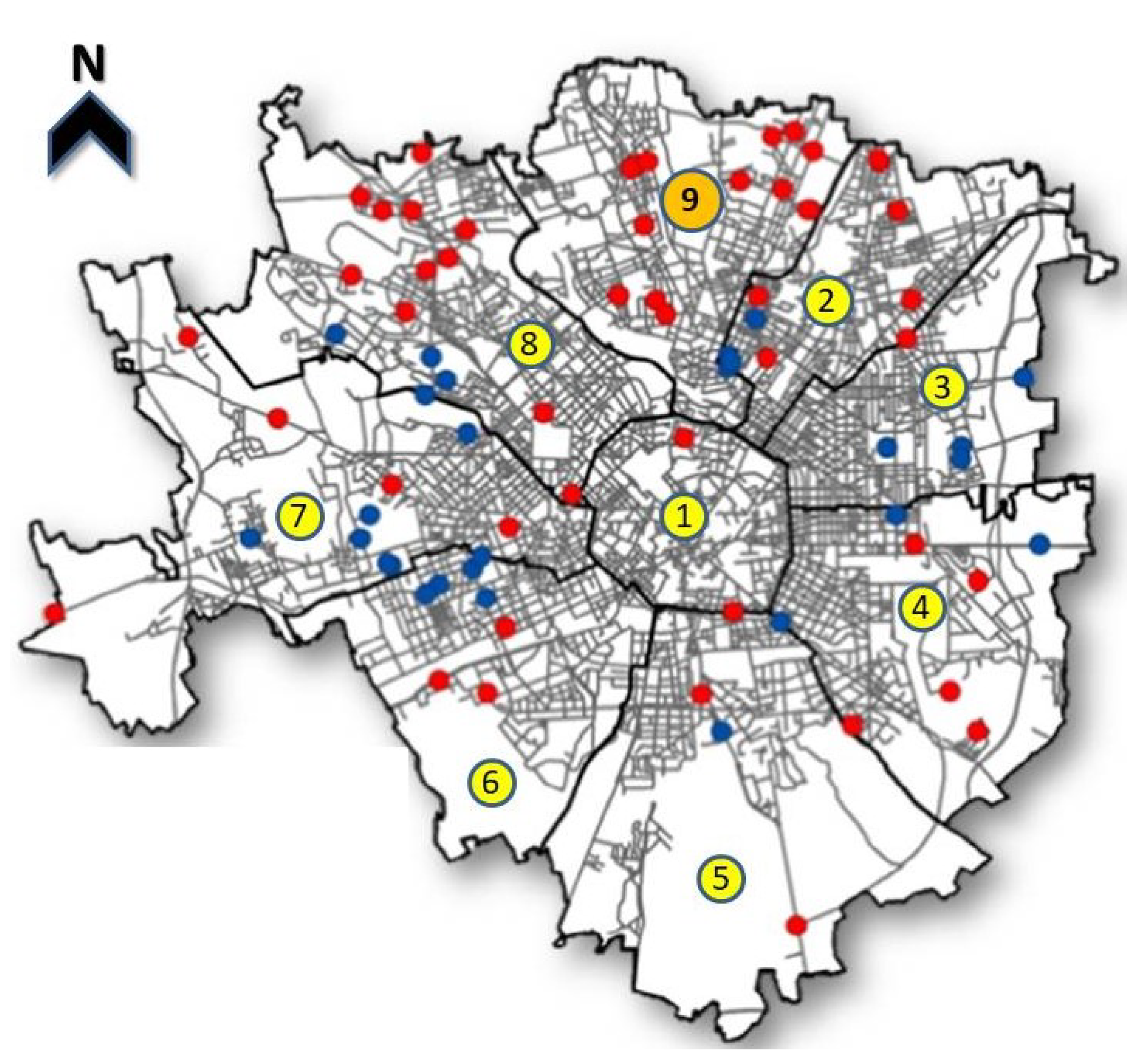
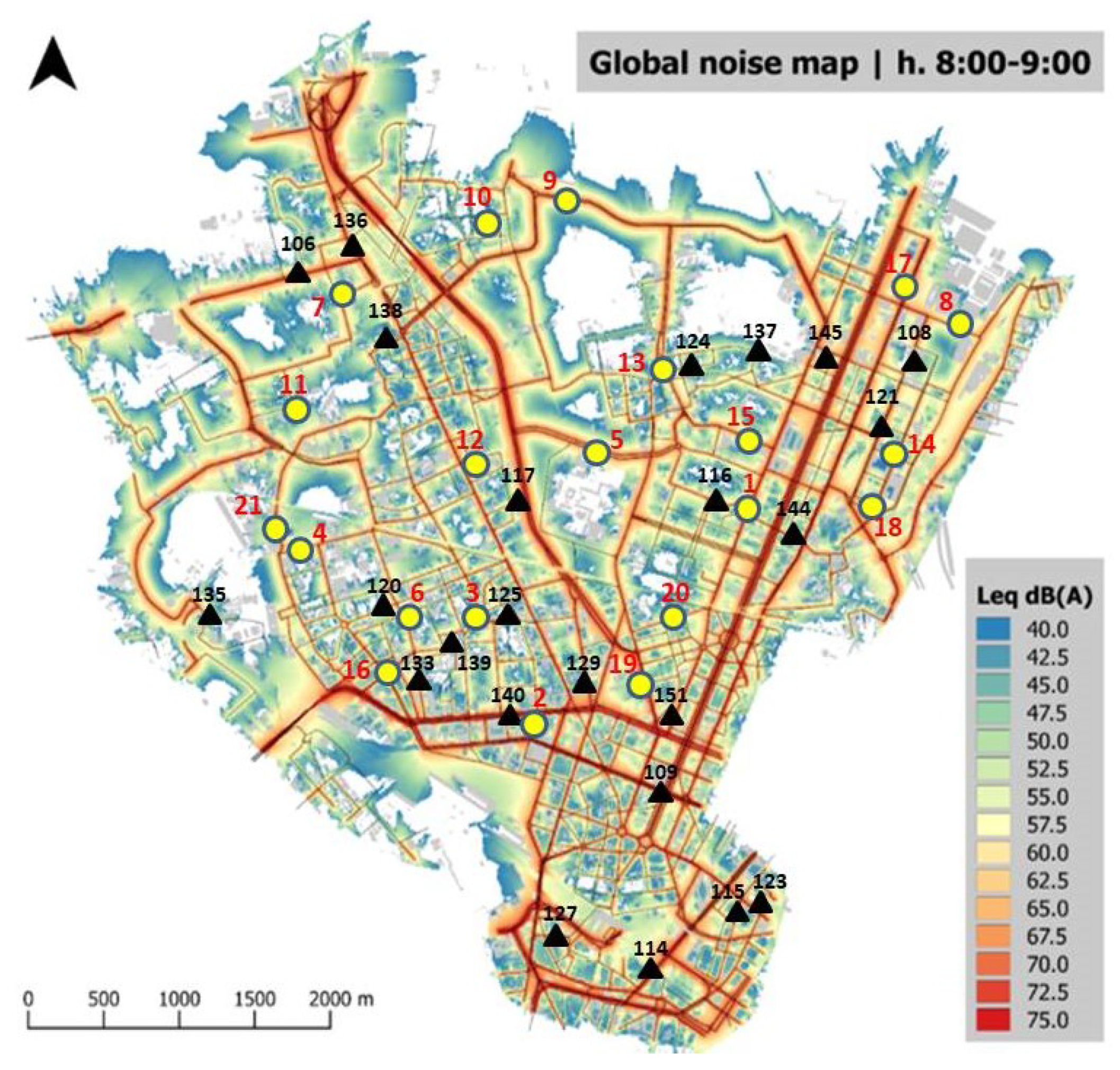
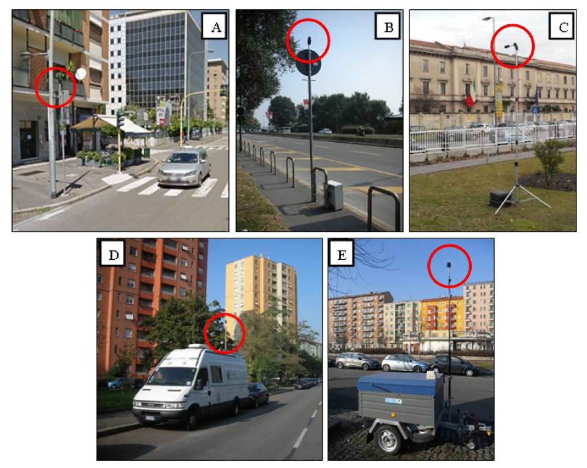
In order to build the method, we rely on measurements of both traffic noise and flow within a large urban zone, in our case the city of Milan [68]. The measurement locations, chosen more or less at random, cover the whole city quite uniformly (see Figure 1). Later, we will describe an optimized procedure to find suitable locations for the measurements, but a random choice is a good one to start with. The type of noise monitoring stations used are illustrated in Figure 2.

The measured signals at 1 s resolution [68] were integrated to obtain the equivalent levels $L_{\mathrm{eq}}^{\left(\tau \right)}(t,s_i)$, where $\tau$ is the temporal interval of interest, $t=n\tau$ ($n\ge 1$) is the time within the day at resolution $\tau$, and $s_i$ (with $i=1,N_m$) is the ith measurement site. In our case, we have a total of $N_m=93$ measurement sites. Regarding the time intervals, we consider $\tau =$ (5, 15, 60) min for most of our analysis.

Since different sites $s_i$ have different traffic noise environments, yielding different absolute $L_{\mathrm{eq}}^{\left(\tau \right)}(t,s_i)$ values, it is convenient to consider the deviations, ${\delta }^{\left(\tau \right)}(t,s_i)$, of the latter with respect to some reference value, $L_{\mathrm{eq}}^{\left({\tau }_0\right)}(t_{\mathrm{ref}},s_i)$, typical of the site location $s_i$, given by

$${\delta }^{\left(\tau \right)}(t,s_i)=L_{\mathrm{eq}}^{\left(\tau \right)}(t,s_i)-L_{\mathrm{eq}}^{\left({\tau }_0\right)}(t_{\mathrm{ref}},s_i).$$

(1)

In this way, we can study traffic noise behavior at different sites by studying the associated deviations along the whole day, which we denote as a normalized noise profile. In our preliminary studies, we take the reference time interval to be ${\tau }_0=1$ h. As a reference level, we considered for each site $s_i$ the daily equivalent level calculated over the period (6:00–10:00 p.m.) [68].

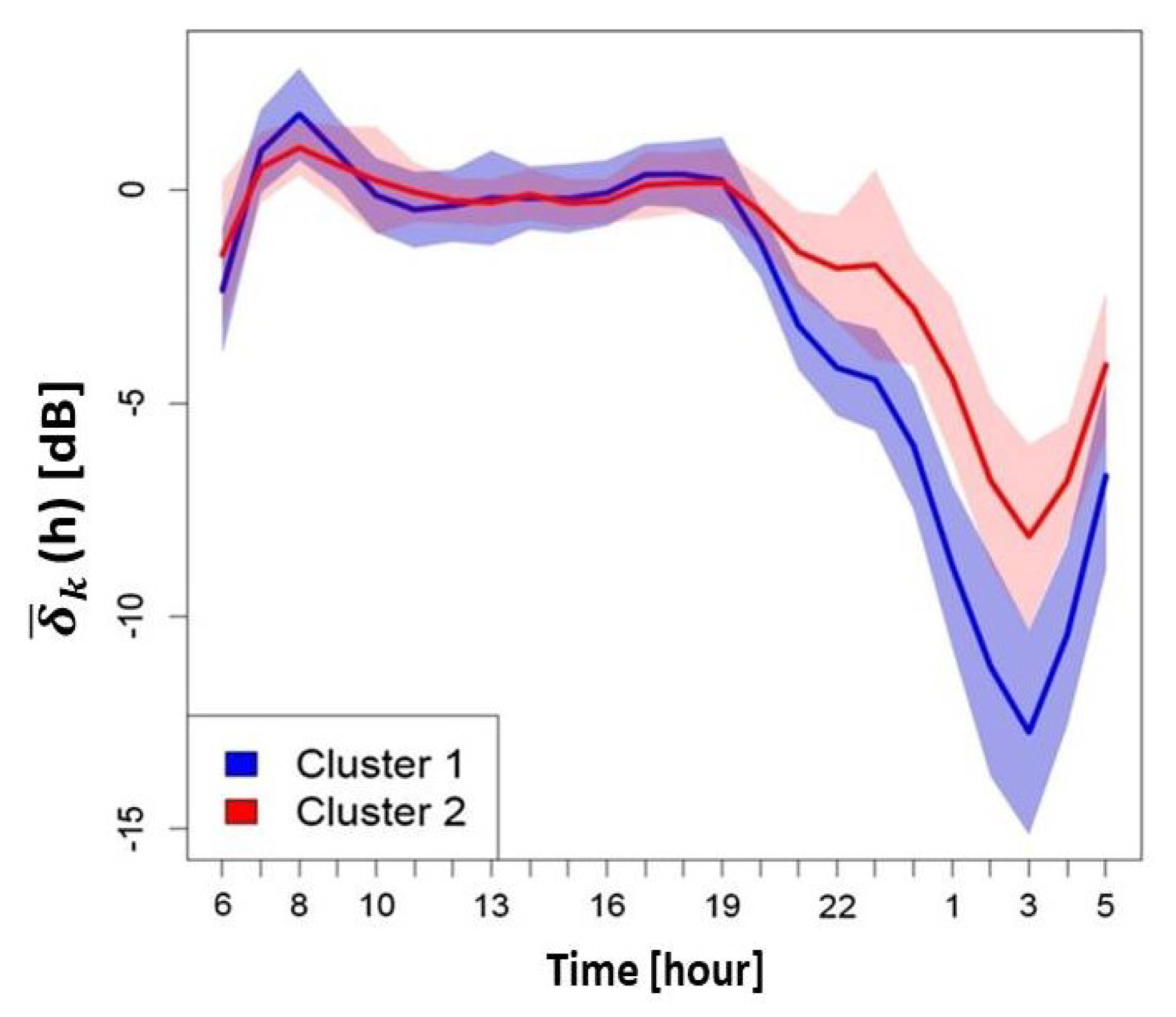
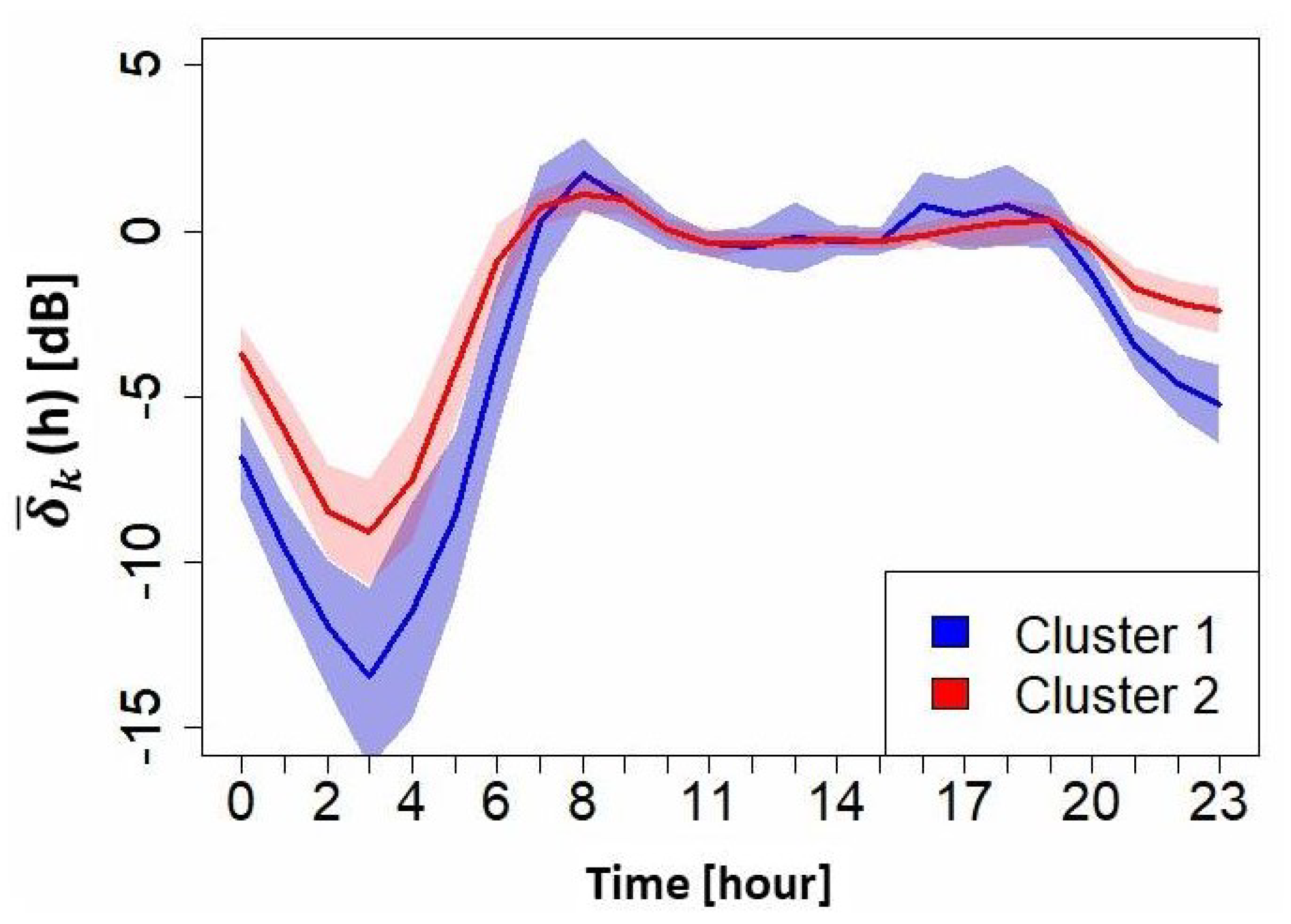
Once the noise profiles have been obtained, a visual analysis shows that strong similarities among profiles occur, suggesting an underlying organization into groups of sites. This organization is different from the standard legislative categorization of roads, as analyzed in some studies [13,14]. For this reason, an unsupervised clustering algorithm was applied to disclose the internal structure of the measurement sites in terms of their normalized noise profiles. The clustering analysis is described in detail in [65,68], where a description in terms of only two clusters is found to be satisfactory. The clusters are labeled with the index $k=1,2$, and the mean hourly cluster profiles denoted as $\overline{{\delta }_k}\left(h\right)$. The results are shown in Figure 3.

Although both clusters display similar mean profiles, they are statistically different [65,68]. Roughly speaking, they differ during the night, as manifested by the larger drop in $\overline{{\delta }_1}\left(h\right)$ with respect to $\overline{{\delta }_2}\left(h\right)$ in Figure 3. Qualitatively, this is due to the fact that traffic flow on road stretches belonging to cluster 1 diminishes much more than on road stretches in cluster 2 during night hours. In other words, cluster 1 roads are lower traffic stretches whose flows decrease more prominently during night periods. On the contrary, road stretches in cluster 2 possess a relatively large traffic flow even during the night. The former represent secondary streets in predominantly residential areas, while the latter main city arteries. In order to characterize the traffic flow of roads, we need to address the issue of vehicles flow within the urban zone. This will require us to define a non-acoustic parameter associated with each road stretch.

2.3.2. Classification of Roads in Large Urban Zones by Their Traffic Flow

Mean hourly values of traffic flow in a given road stretch within the city of Milan are available thanks to the data provided by the EMTA, which is in charge of the traffic mobility management of the city (see [11,65] for further details). The simulation model provides the traffic flow rate, or mean number of vehicles per hour, $F^{\left(1\mathrm{h}\right)}(t,s)$, at hour t of the day and road stretch location s. We have found that it most convenient to take the mean daily total traffic flow, $T_T$, as our candidate to classify traffic flow on road stretches. Specifically, we define our non-acoustic parameter, denoted simply as x, according to

$$x={log}_{10}\left(T_T\right).$$

(2)

It is interesting to observe that one can also apply a clustering method, as we did for the noise in Section 2.3.1, to the traffic flow using the mean daily hourly flow rates produced by the Cadna-EMTA model. We will not discuss this possibility here, but, for details, we refer to [65]. In addition, other issues related to this model can be found in the literature [69,70,82].

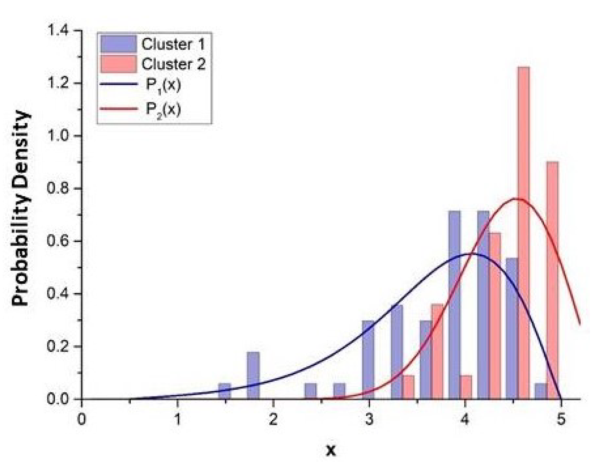
The knowledge of the non-acoustic parameter for each road stretch within the urban zone allows us, in particular, to associate a value of x with each road within the two clusters, denoted as $C_1$ and $C_2$, found from the analysis of traffic noise in Section 2.3.1. Therefore, we are in the position of obtaining the distribution functions, $P_1\left(x\right)$ and $P_2\left(x\right)$, within each cluster. The results are shown in Figure 4.

Since the distribution functions are strongly overlapping, it is more appropriate to consider the probability that a given x value belongs to either $C_1$ or $C_2$, denoted as ${\beta }_1$ and ${\beta }_2$, respectively, i.e.,

$${\beta }_1\left(x\right)=\frac{P_1\left(x\right)}{P_1\left(x\right)+P_2\left(x\right)},{\beta }_2\left(x\right)=\frac{P_2\left(x\right)}{P_1\left(x\right)+P_2\left(x\right)}.$$

(3)

The idea behind this representation is that one can ‘interpolate’ between the normalized mean cluster profiles, $\overline{{\delta }_k}\left(t\right)$, $t=n\tau$, in order to estimate the profile, $\delta (t,x)$, on a road stretch at site s characterized by a non-acoustic parameter $x=x\left(s\right)$, which is given by the relation,

$$\delta (t,x)={\beta }_1\left(x\right)\overline{{\delta }_1}\left(t\right)+{\beta }_2\left(x\right)\overline{{\delta }_2}\left(t\right).$$

(4)

2.3.3. Groups of Roads Defined by Their Daily Total Traffic Flow $T_T$

For building the Dynamap network upon a finite number of dynamical maps, and in particular within the pilot zone 9, it is convenient to define groups of road stretches, denoted as $g_i$, according to their x values, Equation (2). We consider six groups ($i=1,6$) for Z9, which are defined in such a way to contain approximately the same number of road stretches in each group. They are reported in

Table 1. Definition of the six groups of roads, $g_i$ ($i=1,6$), in terms of the non-acoustic parameter, $x={log}_{10}\left(T_T\right)$. Each group has x values within the range indicated in the second row (cf. Figure 4). The corresponding mean values: ${\overline{\beta }}_1\left(g_i\right)=P_1\left(\overline{x}\left[g_i\right]\right)$ and ${\overline{\beta }}_2\left(g_i\right)=P_2\left(\overline{x}\left[g_i\right]\right)=1-{\overline{\beta }}_1\left(g_i\right)$ are indicated in the 3rd and 4th rows, respectively.

Group	${\mathit{g}}_1$	${\mathit{g}}_2$	${\mathit{g}}_3$	${\mathit{g}}_4$	${\mathit{g}}_5$	${\mathit{g}}_6$
$\left[x\right]$	0.0–3.0	3.0–3.5	3.5–3.9	3.9–4.2	4.2–4.5	4.5–5.2
${\overline{\beta }}_1$	0.99	0.81	0.63	0.50	0.41	0.16
${\overline{\beta }}_2$	0.01	0.19	0.37	0.50	0.59	0.84

[83]. Thus, Dynamap [83,86] generalizes the standard categorization of roads discussed in Section 2.3.

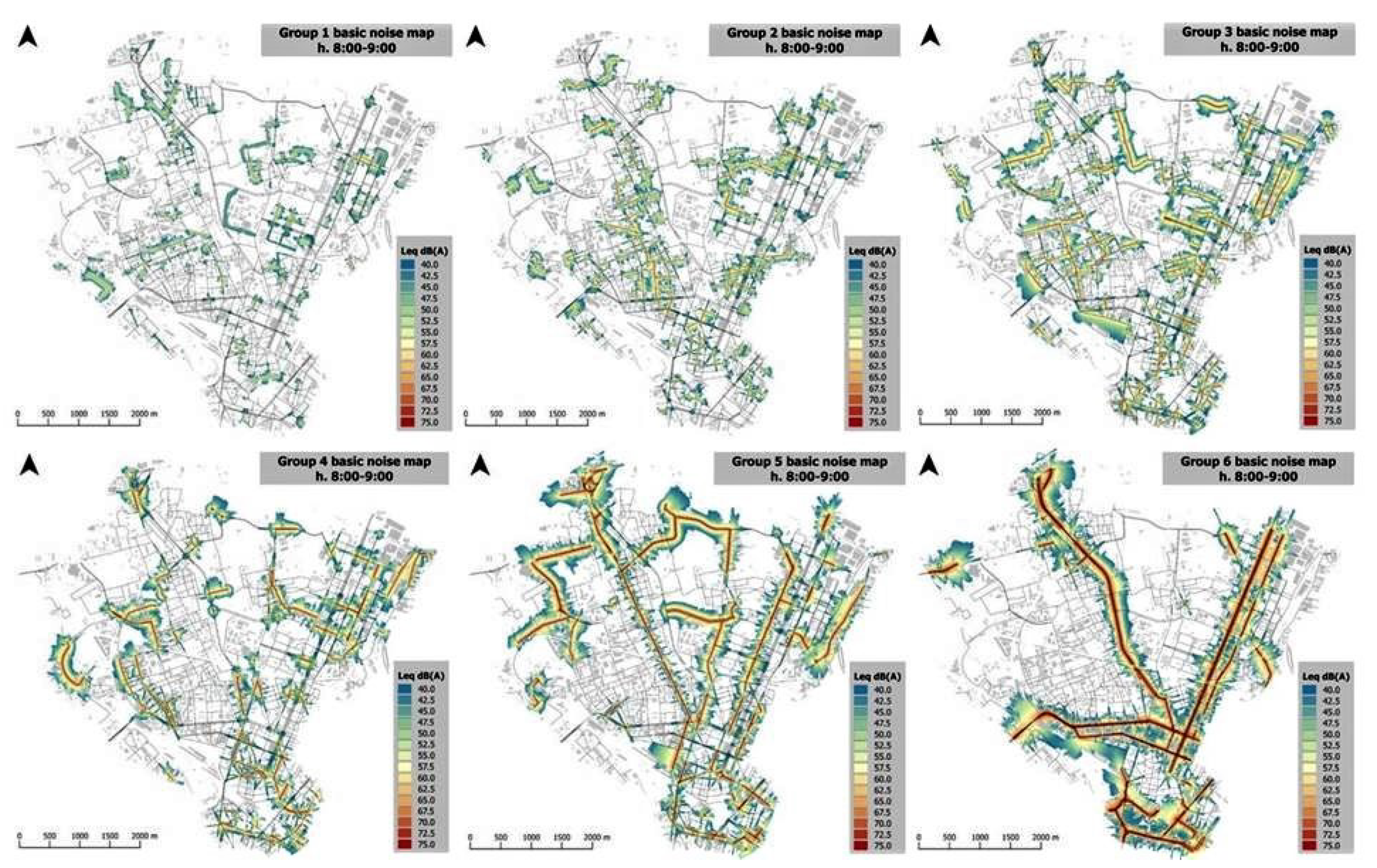
Using the values of traffic noise calculated from the modeled traffic flows (see [86] for details), we display the equivalent noise levels at each road stretch s in zone 9 of the city of Milan, $L_{\mathrm{eq}}^{\left(1\mathrm{h}\right)}(t_{\mathrm{ref}},s)$, obtained at the ‘rush hour’ $t_{\mathrm{ref}}\in$ (8:00–9:00) a.m., for each one of the six groups $g_i$ ($i=1,6$), denoted as the basic traffic noise maps (see Figure 5).

3. Dynamap Approach

The ultimate goal for deploying a network of noise sensors inside an urban zone is the prediction of traffic noise at time t at any road stretch s within the zone. As an attempt to fulfill this goal, we discuss the Dynamap approach, which is illustrated for the pilot zone of the city of Milan, Z9. Therefore, we will assume to have sorted the whole road stretches within Z9 into six groups, as discussed in Section 2.3.3. Each group has associated a dynamical map which can be updated in real time, as illustrated in what follows.

The absolute level $L_{\mathrm{eq}}^{\left(\tau \right)}(t,s)$ at time $t=n\tau$, for the time interval $\tau$, at an arbitrary location s within Z9, can formally be written using the relation [86]

$${\displaystyle L_{\mathrm{eq}}^{\left(\tau \right)}(t,s)=10·{log}_{10}\sum _{i=1}^6{10}^{L_{\mathrm{eq}}^{\left(\tau \right)}(t,s\left(g_i\right))/10},}$$

(5)

where $L_{\mathrm{eq}}^{\left(\tau \right)}(t,s\left(g_i\right))$ represents the contribution of the traffic noise sources on site s from all the road arches within group $g_i$ (not to be confused with the BTNM shown in Figure 5, although we may also refer to these contributions as BTNMs). For our purposes, it is convenient to specify the above relation in the particular case $t=t_{\mathrm{ref}}$ and $\tau =1$ h, where $t_{\mathrm{ref}}\in$ (8:00–9:00) a.m., yielding the reference acoustic equivalent levels,

$${\displaystyle L_{\mathrm{eq}}^{\left(1h\right)}(t_{\mathrm{ref}},s)=10·{log}_{10}\sum _{i=1}^6{10}^{L_{\mathrm{eq}}^{\left(1h\right)}(t_{\mathrm{ref}},s\left(g_i\right))/10},}$$

(6)

for each site s in Z9, in terms of the reference equivalent noise levels contributions from the groups $g_i$ at position s, $L_{\mathrm{eq}}^{\left(1h\right)}(t_{\mathrm{ref}},s\left(g_i\right))$. These quantities can be used back in Equation (5), which now takes the form,

$${\displaystyle L_{\mathrm{eq}}^{\left(\tau \right)}(t,s)=10·{log}_{10}\sum _{i=1}^6{10}^{[{\delta }^{\left(\tau \right)}(t,s\left(g_i\right))+L_{\mathrm{eq}}^{\left(1h\right)}(t_{\mathrm{ref}},s\left(g_i\right))]/10},}$$

(7)

where

$${\delta }^{\left(\tau \right)}(t,s\left(g_i\right))=L_{\mathrm{eq}}^{\left(\tau \right)}(t,s\left(g_i\right))-L_{\mathrm{eq}}^{\left(1h\right)}(t_{\mathrm{ref}},s\left(g_i\right)).$$

(8)

Thus, Equation (8) provides the dynamic counterpart to the stationary map represented by Equation (6).

3.1. The Dynamap Traffic Noise Sensors Network

The main issue of Dynamap is to accurately estimate the variations ${\delta }^{\left(\tau \right)}(t,s\left(g_i\right))$ (Equation (8)) in real time, by relying on the assumption that they do not depend, in a first approximation, on the location s but only on the group $g_i$, i.e., ${\delta }^{\left(\tau \right)}(t,s\left(g_i\right))\cong {\delta }^{\left(\tau \right)}(t,g_i)$. This is based on the empirical fact that the variations ${\delta }^{\left(\tau \right)}(t,s\left(g_i\right))$ do not change appreciably from site to site inside a given group. This means that the group variations ${\delta }^{\left(\tau \right)}(t,g_i)$ can be estimated from a mean value taken over a ‘reduced’ number of sites $s_j\left(g_i\right)$ within $g_i$, i.e.,

$${\delta }^{\left(\tau \right)}(t,g_i)\cong \frac{1}{N\left(g_i\right)}\sum _{j=1}^{N\left(g_i\right)}{\delta }^{\left(\tau \right)}(t,s_j\left(g_i\right)),$$

(9)

where $N\left(g_i\right)$ is the number of road stretches in group $g_i$ considered. In practical circumstances, $N\left(g_i\right)$ can be taken to be much smaller than the total number of sites in $g_i$, allowing us to employ a rather small number of noise sensors to directly measure the noise level variations in real time, where now the sites $s_j\left(g_i\right)$ represent the locations of the Dynamap noise sensors. Finally, the Dynamap prediction for the local equivalent noise level becomes

$${\displaystyle L_{\mathrm{eq}}^{\left(\tau \right)}(t,s)=10·{log}_{10}\sum _{i=1}^6{10}^{[{\delta }^{\left(\tau \right)}(t,g_i)+L_{\mathrm{eq}}^{\left(1h\right)}(t_{\mathrm{ref}},s\left(g_i\right))]/10}.}$$

(10)

For simplicity, we take the same number of sensors within each group, i.e., $N\left(g_i\right)=N_g$, so that the whole Dynamap network is built upon $N_D=6N_g$ noise sensors. In our case, we use $N_g=4$ so that our Dynamap network has just $N_D=24$ fixed stations, which amounts to about 1.2% of the total number of road stretches in Z9 [69,70,82,83]. The problem that arises is how to find a suitable set of locations so that the network can work more efficiently. This question will be considered later below.

3.2. The Group Traffic Noise Variations: ${\delta }^{\left(\tau \right)}(t,g_i)$

3.2.1. Standard Method

This case corresponds to the straightforward use of Equation (9), that is,

$${\delta }^{\left(\tau \right)}(t,g_i)\cong \frac{1}{N_g}\sum _{j=1}^{N_g}{\delta }^{\left(\tau \right)}(t,s_j\left(g_i\right)),$$

(11)

where $N_g=4$ in our case. This simple approach has proved useful to start the Dynamap operations, and it has been found to be accurate in most of the cases studied [69,70,82,83,84,85,86].

3.2.2. The Two Cluster Method: The $\beta$-Model

A little more involved method for estimating ${\delta }^{\left(\tau \right)}(t,g_i)$ consists of the use of all $N_D$ noise stations in the network, instead of only those belonging to group $g_i$ [83,86]. Following the approach discussed in Section 2.3.1, one can classify the measured traffic noise profiles of the noise stations into two clusters, $C_1$ and $C_2$. For both clusters, $k=(1,2)$, one obtains the mean variations ${\overline{\delta }}^{\left(\tau \right)}(t,C_k)$, defined as

$${\overline{\delta }}^{\left(\tau \right)}(t,C_k)=\frac{1}{N_k}\sum _{j=1}^{N_k}{\delta }^{\left(\tau \right)}(t,s_j\left(C_k\right)),$$

(12)

where $N_k$ is the number of stations belonging to cluster $C_k$. Based on Equation (12), one can calculate the mean variations, ${\delta }^{\left(\tau \right)}(t,g_i)$, associated with group $g_i$, as follows:

$${\delta }^{\left(\tau \right)}(t,g_i)={\overline{\beta }}_1\left(g_i\right){\overline{\delta }}^{\left(\tau \right)}(t,C_1)+{\overline{\beta }}_2\left(g_i\right){\overline{\delta }}^{\left(\tau \right)}(t,C_2).$$

(13)

The values of ${\overline{\beta }}_k\left(g_i\right)$ can be obtained from Table 1. The actual implementation of the noise variations, ${\delta }^{\left(\tau \right)}(t,s_j\left(C_k\right))$, measured by the sensors $s_j\left(C_k\right)$ in cluster k, is specified in the next Section 3.3.

3.3. The Dynamap Network for Z9: Implementation, Location, and Operation

We specify next how to implement the noise sensors data acquisition (Section 3.3.1), location (Section 3.3.2), and operation (Section 3.3.3).

3.3.1. The Sensors Implementation and ANED

The basic equation for predicting the traffic noise level at a site s is given by Equation (10), where the group noise variations, ${\delta }^{\left(\tau \right)}(t,g_i)$, are a function of the single sensors acquired data, ${\delta }^{\left(\tau \right)}(t,s_j\left(g_i\right))$, as discussed in Section 3.2. In the realm of Dynamap, we define the latter as follows:

$${\delta }^{\left(\tau \right)}(t,s_j\left(g_i\right))=L_{\mathrm{eq}}^{\left(\tau \right)}{(t,s_j\left(g_i\right))}_{\mathrm{meas}}-L_{\mathrm{eq}}^{\left(1h\right)}{(t_{\mathrm{ref}},s_j\left(g_i\right))}_{\mathrm{calc}},$$

(14)

where $L_{\mathrm{eq}}^{\left(\tau \right)}{(t,s_j\left(g_i\right))}_{\mathrm{meas}}$ are the measured acoustic levels by the sensor at the location $s_j\left(g_i\right)$, and $L_{\mathrm{eq}}^{\left(1h\right)}{(t_{\mathrm{ref}},s_j\left(g_i\right))}_{\mathrm{calc}}$ the calculated reference acoustic levels obtained at the rush hour $t_{\mathrm{ref}}\in$ (8:00–9:00) a.m. (see Figure 5 for details). These variations, which are of the same form as in Equation (8), can be used then either in Equation (11), or in Equations (12) and (13), to obtain the group variations ${\delta }^{\left(\tau \right)}(t,g_i)$.

Due to the complexity of the urban noise scenario, both in space and time, an automated update of the noise maps is required. This is essentially the whole idea of the Dynamap system. One of the issues of the automated system is the content of the detected noise level that can include, in addition to the main noise source, i.e., the road traffic, the contribution of additional noise sources present in the mapping area. If these additional sources of noise are not filtered out, the resulting maps would not constitute a faithful reflection of the acoustic impact of road infrastructures. For this reason, it is necessary to endow the Dynamap system with the ability to discern between road traffic noise and other types of acoustic events (e.g., aircrafts, industries, works on the road, people talking, etc.), to exclude the latter from the noise level computation. To this end, an anomalous noise event detection (ANED) algorithm was developed [71,76,84,85]. This algorithm operates on the audio stream captured by the acoustic sensors and identifies the presence of acoustic events unrelated to road traffic, activating an alert signal to exclude the corresponding audio passages from the computation of noise levels.

The design of the ANED algorithm follows a “detection-by-classification” approach, consisting of the binary classification of sequential audio segments as either “road traffic noise” or “anomalous noise event”. The algorithm is able to discern three main signal categories: road traffic noise, background city noise, and anomalous events. This latter class is further divided into 18 subtypes of events, such as people talking, music in car or in the street, or noise caused by tramways or trains, etc. The ANED algorithm is trained, validated, and tested using a data set containing samples of both road traffic and anomalous noise events taken from real environmental contexts [71,72,73,74,75,76,85].

3.3.2. The Sensor Locations in Z9

As mentioned in Section 3.1, we have at our disposal 24 sensor stations which need to be distributed within Z9 in an optimized fashion. The natural choice is to get an equal number of sensors per group that is $N_g=4$, and somehow well separated from each other. To this end, we have first plotted all road groups, $g_i$ (shown separately in Figure 5), together in Figure 6, so that one can get a full picture on the spatial distribution of equivalent levels, $L_{\mathrm{eq}}^{\left(1\mathrm{h}\right)}(t_{\mathrm{ref}},s)$, in the pilot zone Z9 [86,87,88,89,90]. The selection of sensor locations is shown in Figure 6 by the full black triangles, and the corresponding addresses are reported in

Table 2. Location of the 24 Dynamap noise monitoring stations (cf. Figure 6). For each sensor, the code number, group index $g_i$ (within parenthesis), and name of the street are reported [91].

Code (${\mathit{g}}_{\mathit{i}}$)	Address	Code (${\mathit{g}}_{\mathit{i}}$)	Address
135   (1)	Via Lambruschini	121   (4)	Via Piero e Alberto Pirelli
137   (1)	Via Maestri del Lavoro	127   (4)	Via Quadrio
139   (1)	Via Bruni	129   (4)	Via Crespi
144   (1)	Via D’Intignano	138   (4)	Via Novaro
108   (2)	Via Piero e Alberto Pirell i	106   (5)	Via Litta Modignani
124   (2)	Via Grivola	123   (5)	Via Galvani
125   (2)	Via Abba	136   (5)	Via Comasina
145   (2)	Via Fratelli Grimm	151   (5)	Via Veglia
115   (3)	Via Fara	109   (6)	Viale Stelvio
116   (3)	Via Moncalieri	114   (6)	Via Melchiorre Gioia
120   (3)	Via Baldinucci	117   (6)	Viale Fermi
133   (3)	Via Maffucci	140   (6)	Viale Jenner

, while the yellow circles correspond to the sites where additional measurements have been performed for validation purposes (see Section 4.1).

3.3.3. The Network Operation: Standard Method and the $\beta$-Model

The Dynamap network is expected to work continuously [12], yielding integrated equivalent noise levels at intervals $\tau =(5,15,60)$ min. Extensive hourly data have been downloaded and the 24 time series analyzed according to the clustering procedure discussed in Section 2.3.1. The corresponding mean normalized hourly cluster profiles, $\overline{{\delta }_k}\left(h\right)$, $k=1,2$ (see Equation (12)), are displayed in Figure 7.

The cluster compositions are reported in

Table 3. Monitoring sensors information: Code, group membership, non-acoustic parameter $x=log\left(T_T\right)$, and cluster membership. The cluster compositions are: (Cluster 1) 12 sensors; (Cluster 2) 12 sensors [91]. Note that sensors in groups: $g_2$, $g_3$, $g_4$, are shared among the two clusters.

Sensor Code	Group ${\mathit{g}}_{\mathit{i}}$	x	Cluster	Sensor Code	Group ${\mathit{g}}_{\mathit{i}}$	x	Cluster
135	1	2.89	1	108	2	3.06	2
137	1	1.90	1	120	3	3.74	2
139	1	1.13	1	121	4	4.06	2
144	1	2.94	1	129	4	3.94	2
124	2	3.50	1	106	5	3.90	2
125	2	2.69	1	123	5	4.30	2
145	2	3.42	1	136	5	4.21	2
115	3	3.58	1	151	5	4.40	2
116	3	3.60	1	109	6	4.75	2
133	3	3.75	1	114	6	4.58	2
127	4	3.90	1	117	6	4.85	2
138	4	4.19	1	140	6	4.70	2

, together with the sensor codes, groups $g_i$, and values of the local non-acoustic parameter x. As one can see from these results, Cluster 1 is built predominantly upon groups 1, 2, and 3, while Cluster 2 on groups 5 and 6. Stations located within group 4 are present with equal numbers in both clusters. This is a consequence of the partial overlap of the two main clusters, as we already found in Figure 4. The strong similarity of both results is noteworthy, Figure 3 and Figure 7, suggesting that the 24 sensors yield an accurate representation of the two mean noise cluster behaviors. Once these mean variations are known, one can apply Equation (13) in order to obtain the mean group noise variations, ${\delta }^{\left(\tau \right)}(t,g_i)$. In principle, one can run the network based on the standard approach using Equation (11), which is also useful in the preliminary stages of operation.

4. Results

In Section 4.1, we discuss additional measurements for the assessment of the group components. The validation of Dynamap predictions is discussed in Section 4.2, followed by the issue of cross-correlations between sensors noise data in Section 4.3. The latter is an attempt to provide a guideline for optimizing the choice of sensor locations within the urban zone. Finally, in Section 4.4, results of correlations of Dynamap predictions with measurements are presented.

4.1. Additional Measurements Sites: Assessment of the Group Components

Measurements of both traffic noise and vehicle flow have been performed in randomly chosen locations within Z9 in order to validate the Dynamap predictions. The analysis is also aimed at determining absolute values of the errors involved in the predictions, and from the detail comparison with the measurements being able to evaluate the limitations of the method. The locations and the corresponding groups are reported in

Table 4. Location of the measurement sites (cf. Figure 6). The group index $g_i$ is indicated in parentheses [91].

Site	Address	Site	Address	Site	Address
1 (5)	Via Suzzani	8 (3)	Via Chiese	15 (4)	Via Gregorovius
2 (2)	Via Bernina	9 (5)	Via Moro	16 (4)	Via Catone
3 (3)	Via Ciaia	10 (1)	Via Marchionni	17 (6)	V.le Sarca
4 (3)	Via Cosenz	11 (1)	Via Gabbro	18 (1)	Via Boschi Di Stefano
5 (5)	Via Majorana	12 (2)	Via Pastro	19 (6)	Via Murat
6 (3)	Via Maffucci	13 (4)	Via Bauer	20 (1)	Via Sarzana
7 (2)	Via Ippocrate	14 (2)	Via Polvani	21 (3)	Via Cosenz

.

In

Table 5. The calculated total reference levels (BTNM), $L_{\mathrm{eq}}^{\left(1h\right)}(t_{\mathrm{ref}},s)$, at 13 arbitrarily chosen sites s of pilot Zone 9 (cf. Table 4). The level contributions from each group, $L_{\mathrm{eq}}^{\left(1h\right)}(t_{\mathrm{ref}},s\left(g_i\right))$, are reported in columns (4th–9th) [86]. All levels are expressed in dB. The underscored values correspond to the largest contribution to each reference level. Here, the number $0.0$ stands for vanishingly small values.

Site	${\mathit{g}}_{\mathit{i}}$	${\mathit{L}}_{\mathbf{eq}}^{\left(1\mathit{h}\right)}$	$\mathit{s}\left({\mathit{g}}_1\right)$	$\mathit{s}\left({\mathit{g}}_2\right)$	$\mathit{s}\left({\mathit{g}}_3\right)$	$\mathit{s}\left({\mathit{g}}_4\right)$	$\mathit{s}\left({\mathit{g}}_5\right)$	$\mathit{s}\left({\mathit{g}}_6\right)$
1	5	64.0	21.7	44.9	54.3	55.0	62.7	37.7
2	2	65.8	12.0	64.6	15.0	15.0	15.0	59.6
3	3	63.6	0.0	56.1	62.7	0.0	0.0	0.0
4	3	60.8	17.3	25.4	59.9	49.2	51.5	0.0
5	5	68.0	29.7	25.9	32.3	29.4	68.0	33.8
6	3	64.3	38.8	45.4	64.2	34.2	26.9	28.0
7	2	59.2	24.1	58.1	51.4	17.8	42.2	45.6
8	3	55.4	21.8	22.0	54.1	49.6	30.4	30.1
9	5	62.6	8.5	32.0	34.7	43.0	62.5	0.0
10	1	45.2	38.1	43.6	26.6	25.6	33.0	28.3
11	1	55.5	55.1	20.8	32.0	37.8	43.0	0.0
12	2	62.1	42.3	61.8	24.1	20.4	48.3	41.0
13	4	68.2	41.2	53.0	38.2	68.0	41.2	38.5

, we report calculations of the contributions from different groups, $L_{\mathrm{eq}}^{\left(1h\right)}(t_{\mathrm{ref}},s\left(g_i\right))$, to the local equivalent level, $L_{\mathrm{eq}}^{\left(1h\right)}(t_{\mathrm{ref}},s)$, at selected locations s corresponding to some of the measurements sites listed in Table 4. These results have been obtained by setting ${\delta }^{\left(\tau \right)}(t,g_i)=0$ in Equation (10), since we are dealing with the static maps (BTNMs) at the reference time $t=t_{\mathrm{ref}}$.

As one can see from Table 5, the major contribution to the local site level comes from the group $g_i$ which the site belongs to. This can be clearly seen by comparing the values of $L_{\mathrm{eq}}^{\left(1h\right)}(t_{\mathrm{ref}},s\left(g_i\right))$ for different groups. For example, for Site 1, which belongs to group $g_5$, the most significant contribution comes from $L_{\mathrm{eq}}^{\left(1h\right)}(t_{\mathrm{ref}},s\left(g_5\right))$. However, each local site level is subject to the influence of nearby streets through other groups, as it is apparent from Table 5. In particular, for Site 10, the maximum contribution is due to $L_{\mathrm{eq}}^{\left(1h\right)}(t_{\mathrm{ref}},s\left(g_2\right))$, although the site belongs to group $g_1$. This is the result of the complex noise environment around Site 10, and it may be expected to have further consequences regarding the model predictions.

4.2. Validation of Dynamap: Sites 10 and 12

For the validation of Dynamap predictions, we have studied all the 21 measurement sites reported in Table 4. As an illustration, we discuss here only the cases of Sites 10 and 12. The former belongs to group $g_1$ and the latter to $g_2$. Before discussing traffic noise results, we present a comparison between traffic flow measurements, at these two locations, and the predictions from the traffic flow model (see [86] for more details on the EMTA traffic flow model). The reason for testing the traffic flow model is because it plays a prominent role in the Dynamap approach through the BTNMs, as one can see from Equation (10). The two chosen sites (10 and 12) provide examples of the difficulties that one finds in this approach (see Figure 8), and also suggest ways of improving Dynamap predictions.

In Figure 8, we see the two possible behaviors typically found from our validation analysis. In Site 10 (Figure 8a), one can see that the traffic model drastically underestimates the actual traffic flow. This is because Site 10 belongs to the lowest flow group in Z9, where the model is less accurate. The latter is indeed ‘tuned’ to work better for high traffic flow road stretches. The model predictions for Site 12 (Figure 8b) are, in contrast, in very good agreement with the measurements. We will see below the consequences these outcomes have on the local traffic noise predictions.

In Figure 9a (upper and lower parts), we compare the Dynamap predictions, Equation (10), for Sites 10 and 12 with the actual measurements. We find in both cases that the absolute noise levels, $L_{\mathrm{eq}}^{\left(1h\right)}(t,s)$, as a function of hour of day, depart from the measured ones essentially by a constant amount. For Site 10, the prediction underestimates the experimental values, while, for Site 12, Dynamap overestimates it. For both sites, the discrepancies are higher during the day time than during night hours. Notice also the wild variation in the statistical errors (shown as the color bands in Figure 9), as a function of hour of the day. In particular, during the day time (7:00–9:00 p.m.), the statistical error is rather small, i.e., ∼1 dB, after averaging over all sites in the group, whereas in the evening-night time (9:00 p.m.–7:00 a.m.), the error bands are much larger, i.e., ∼(2–4) dB on average, due to the high variability of traffic flow and associated noise during night hours.

These considerations led us to study the presence of systematic errors inherent in the Dynamap approach. For instance, it is clear from our basic definition of the variations in Equation (14), ${\delta }^{\left(\tau \right)}(t,s)$, that a small error in the reference level, $L_{\mathrm{eq}}^{\left(1h\right)}(t_{\mathrm{ref}},s)$, may result in a shift of the total equivalent level prediction by quite an amount. This discrepancy can have two origins: one may be a poor estimation of the traffic flow at site s at time $t_{\mathrm{ref}}$ by the traffic model, and a second, an inaccurate determination of the noise contributions from the different groups at site s.

In order to elucidate these issues further, one can calculate the deviations of the predictions from the measured ones, for both the equivalent hourly noise levels, $L_{\mathrm{eq}}^{\left(1h\right)}(t_{\mathrm{ref}},s)$, and the logarithm of hourly traffic flows, $log{F}^{\left(1h\right)}(t_{\mathrm{ref}},s)$, at time $t_{\mathrm{ref}}$ at different sites s. These are defined, respectively, as,

$$\begin{array}{ccc}\hfill {\epsilon }_{\mathrm{Leq}}(t_{\mathrm{ref}},s)& =& \frac{L_{\mathrm{eq}}^{\left(1h\right)}{(t_{\mathrm{ref}},s)}_{\mathrm{calc}}-L_{\mathrm{eq}}^{\left(1h\right)}{(t_{\mathrm{ref}},s)}_{\mathrm{meas}}}{L_{\mathrm{eq}}^{\left(1h\right)}{(t_{\mathrm{ref}},s)}_{\mathrm{meas}}},\hfill \end{array}$$

(15)

$$\begin{array}{ccc}\hfill {\epsilon }_{\mathrm{Flw}}(t_{\mathrm{ref}},s)& =& \frac{log{F}^{\left(1h\right)}{(t_{\mathrm{ref}},s)}_{\mathrm{calc}}-log{F}^{\left(1h\right)}{(t_{\mathrm{ref}},s)}_{\mathrm{meas}}}{log{F}^{\left(1h\right)}{(t_{\mathrm{ref}},s)}_{\mathrm{meas}}}.\hfill \end{array}$$

(16)

The above values for ${\epsilon }_{\mathrm{Leq},\mathrm{Flw}}(t_{\mathrm{ref}},s)$ can be averaged over all sites s belonging to the same group $g_i$, and, in addition, an average can be performed over different hours of the day. In the latter case, we will denote the resulting mean values as ${〈{ϵ}_{\mathrm{Leq}}〉}_{\mathrm{X}}$, where the subscript X indicates the type of average employed. A preliminary analysis of correlations between values of ${\epsilon }_{\mathrm{Leq}}(t,s)$ and ${\epsilon }_{\mathrm{Flw}}(t,s)$ have been performed [86], from which empirical ‘corrections’, denoted with the subscript C, have been obtained in order to improve the performance of Dynamap. The results are shown in Figure 9b, for both Sites 10 and 12, suggesting that some improvement can be obtained in this way.

Despite the presence of significant deviations from the measured values still observed in Figure 9, the analysis extended to other available sites, belonging to groups ($g_1-g_6$), yields a more optimistic picture. This can be appreciated from the results reported in

Table 6. Mean local deviations (in dB) of Dynamap predictions from measurements at different sites. The codes of the measurement sites (first column) are indicated by single numbers (see Table 4). The group index $g_i$ is given for each site (second column). The remaining three columns report the mean deviations: ${〈{ϵ}_{\mathrm{Leq}}〉}_{\mathrm{N}}$ obtained without systematic error corrections, ${〈{ϵ}_{\mathrm{Leq}}〉}_{\mathrm{C}}$ obtained after systematic error corrections have been applied, and ${〈{ϵ}_{\mathrm{Leq}}〉}_{\mathrm{M}}$ corresponding to the median average of the corrected predictions [91].

Site	${\mathit{g}}_{\mathit{i}}$	${〈{\mathit{ϵ}}_{\mathbf{Leq}}〉}_{\mathbf{N}}$	${〈{\mathit{ϵ}}_{\mathbf{Leq}}〉}_{\mathbf{C}}$	${〈{\mathit{ϵ}}_{\mathbf{Leq}}〉}_{\mathbf{M}}$
10	1	5.0	5.2	5.2
11	1	4.5	4.0	4.1
18	1	6.4	6.1	6.1
20	1	5.3	5.5	5.6
7	2	1.9	4.0	2.9
12	2	7.8	2.5	3.8
14	2	2.8	3.1	1.6
3	3	1.8	2.3	2.5
4	3	2.1	1.5	2.0
6	3	4.2	4.5	5.9
21	3	1.8	1.5	0.7
13	4	4.1	2.0	0.8
15	4	3.3	2.6	1.3
16	4	8.4	2.6	4.2
1	5	4.5	3.0	4.4
5	5	1.9	2.4	1.2
9	5	1.4	1.9	1.0
19	6	3.4	1.3	1.3

. Quite illustrative are the mean group values reported in

Table 7. Mean group deviations (in dB) of Dynamap predictions from measurements, for groups ($g_1-g_6$). Here, ${〈{ϵ}_{\mathrm{Leq}}〉}_{\mathrm{N}}$ are the deviations obtained without systematic error corrections, ${〈{ϵ}_{\mathrm{Leq}}〉}_{\mathrm{C}}$ those obtained with systematic error corrections, and ${〈{ϵ}_{\mathrm{Leq}}〉}_{\mathrm{M}}$ the median of the corrected group predictions [91].

${\mathit{g}}_{\mathit{i}}$	${〈{\mathit{ϵ}}_{\mathbf{Leq}}〉}_{\mathbf{N}}$	${〈{\mathit{ϵ}}_{\mathbf{Leq}}〉}_{\mathbf{C}}$	${〈{\mathit{ϵ}}_{\mathbf{Leq}}〉}_{\mathbf{M}}$
1	5.3	5.1	5.2
2	4.2	3.2	2.8
3	2.5	2.5	2.8
4	5.3	2.4	2.1
5	2.6	2.4	2.2
6	3.4	1.3	1.3

, yielding mean deviations below 3 dB in most cases. Again, the largest discrepancies occur for $g_1$, as expected.

4.3. Correlations between Sensor Locations: How to Optimize the Network

Thus far, we have discussed how the Dynamap network can be constructed, presenting detailed discussions of its design, and how its predictions can be assessed by reporting a number of tests for its validation. The general question arises, a posteriori, of how the design of the network can be optimized further. The way to do it is closely related to the concept of correlations among the noise station measurements. The idea is rather simple: one wishes to reduce to a minimum the amount of redundant information registered by the different stations. In other words, their locations should be identified such that they can collect as much distinct information as possible about the traffic noise within the urban zone.

To this end, we study the sensor variations, ${\delta }^{\left(\tau \right)}(t,s_j\left(g_i\right))$ (Equation (14)), at different time intervals $\tau =(5,10,15,30,60)$ min, over a period of five consecutive working days, thus creating 24 contemporary times series for each value of $\tau$. To determine the degree of correlation between, say, sensors $s_j$ and $s_{j^{\prime }}$, we calculate the Pearson’s correlation coefficient (see, e.g., [60]), given by

$$\rho (j,j^{\prime })=\frac{\mathrm{cov}(j,j^{\prime })}{{\sigma }_j{\sigma }_{j^{\prime }}},$$

(17)

where cov($j,j^{\prime }$) is the covariance between times series j and $j^{\prime }$, defined in the standard fashion as the mean value of the product of the deviations from their mean values, and ${\sigma }_{j,j^{\prime }}$ are the corresponding standard deviations of the time series. In this way, we can study both intragroup correlations (same sensor group indexes $g_i$) or intergroup ones (different $g_i$’s).

To study the noise correlations among the 24 sensors using Equation (17), we employ two normalization procedures:

• (P1) From each time series, we remove the hourly median value. In this way, we obtain what we called a de-trended time series.
• (P2) From each time series, we remove the mean level, $〈L_{\mathrm{eq}}^{\left(1h\right)}(t,s)〉$, calculated between 6:00–10:00 p.m. This normalization procedure retains both high and low frequency fluctuations.

An illustrative example of each procedure is shown in Figure 10, for the noise station $s136$ at time interval $\tau =5$ min. To be noted is that, for P1, the resulting profile is quite flat over the day, while, for P2, it clearly retains the typical shape observed in the original noise profiles (see, e.g., Figure 7).

The median correlation coefficients obtained for P1 and P2 are shown in Figure 11, as a function of time interval $\tau$. The reported ‘error’ bands correspond to the median absolute deviation, MAD $=\mid x_i-\tilde{X}\mid$, where $\tilde{X}=$ median $\left(X\right)$ and $X\equiv \left(x_1,\cdots ,x_n\right)$ is a generic time series.

As one can see from Figure 11 in the case of P1, the median correlation coefficients over all stations $s_j$ are quite small (∼0.1–0.2). This is because procedure P1 removes all long period fluctuations, thus only high frequency fluctuations remain (see [92,93], where a power-spectrum analysis in the frequency domain has been performed). These results suggest that, on average, short time (high frequency) correlations among stations are low, as we expect from a ‘well-designed’ network. The situation changes a bit if one looks in more detail to intra-group correlations separately. They can be seen in the lower panel of Figure 11 (P1). Now, all groups behave similarly as the global mean, except for group $g_5$. This is an indication that one or more stations inside $g_5$ need to be moved to other more suitable locations. Such analysis remains to be performed.

The situation for procedure P2 is quite different (see Figure 11 (P2)), providing useful information on Dynamap performance. Since P2 retains long-time fluctuations, we can actually observe that sensors remain quite correlated on long-times, a feature that is at the basis of the good performance of Dynamap. In particular, the upper panel shows that the median correlation coefficient grows to 0.8 for $\tau =60$ min, suggesting that all noise sensors respond similarly to fluctuations around the mean hourly noise profiles. This result supports a posteriori our approach based on the two-cluster mean profiles discussed in previous sections. The lower panel of Figure 11 (P2) confirms that all groups behave the same at all time intervals $\tau$.

4.4. Correlations of Dynamap Predictions with Measurements

In the following, we discuss the tests performed to evaluate Dynamap predictions based on Equation (10). The locations of the measurement sites are reported in Table 4, and have been shown by the filled yellow circles within Z9 in Figure 6. The measurement sites have been selected in order to test the system in complex scenarios where the noise from roads belonging to different groups may contribute to the local noise level. We have used the updating times: $\tau =(5,10,15,30,60)$ min, and all time series have been normalized according to procedure P2. The validation of Dynamap predictions are based on the calculation of the associated correlation coefficients, Equation (17), between predictions and measurements. The calculations have been performed between

• Case 1: A single measurement at site $s_j$ with the corresponding Dynamap prediction.
• Case 2: The mean group values, $〈L_{\mathrm{eq}}^{\left(\tau \right)}(t,s\left(g_i\right))〉$, for the measurements and the mean Dynamap predictions, for all groups $g_i$.

The results are shown in Figure 12.

As one can see, the correlation coefficients systematically increase with the integration time $\tau$, but, at low times, such as for $\tau =5$ min and $\tau =10$ min in Case 1, the correlations are quite low. However, as it is apparent from Figure 12, Dynamap predictions present good correlation results with measurements, especially at higher integration times ($\tau >10$ min). This result can be expected since high updating times $\tau$ reduce high frequency fluctuations letting low frequency periodicities emerge. Furthermore, correlation performance is enhanced at all integration times when, within each group, one computes the correlation coefficient between mean Dynamap predictions and corresponding mean values of measurements. This is consistent with the fact that Dynamap noise description has a statistically-based approach and, therefore, its performance is enhanced when averaging over a sufficient number of observations.

The results shown in Figure 12 are quite illustrative as they indicate a typical range of variability of Dynamap predictions from the real measurements. It can be used as a starting point also for the search of better site locations of the fixed noise stations within Z9. An attempt can also be made to connect these correlation results with the mean noise level deviations reported in Table 6 and Table 7. This remains to be investigated.

5. Conclusions

Dynamap is the first automatic monitoring system, based on customized low cost sensors and a software tool implemented on a general purpose GIS platform, performing the update of noise maps in real time (dynamic noise maps) on a large urban area. The update of noise maps is accomplished by scaling pre-calculated basic noise maps. The latter are selected and scaled using the information retrieved from low cost sensors continuously measuring the sound pressure levels of the primary noise sources present in the mapping area. A complete basic noise map covering the entire survey area is calculated and saved for each source. Scaled basic noise maps of each primary source are then energetically summed up to provide the overall noise map of the area. In this way, the need for several and expensive software license is extremely reduced and limited only to the preparation of the basic noise maps.

The proposed method of noise mapping is essentially a statistically-based approach, whose predictive power over the entire road network relies on the assignment of a non-acoustic parameter to each road stretch. This is an essential requirement that must be complied to generalize Dynamap project to other cities. The non-acoustic parameter must show a high degree of correlation with the road traffic noise level. In the case of the District 9 (Z9) of the city of Milan, the correlation was about (60–65)%. In terms of accuracy, the predictive capability of the Dynamap scheme is mainly associated with the related accuracy of the chosen non-acoustic parameter. For this reason, a poor accuracy in the latter is directly reflected on the noise prediction error. For example, in the case in which the non-acoustic parameter is provided by a road traffic flow model (here taken as the total daily traffic flow), eventual errors in the traffic noise predictions can be traced back to a discrepancy between the measured and the model predicted hourly traffic flows. As a by-product of Dynamap, the use of the non-acoustic parameter generalizes the standard concept of road categorization, which has been used so far in most applications.

The overall mean prediction error of Dynamap for Z9 is estimated to be about 3 dB, which can be seen as a very promising result for most practical applications. Specifically, Dynamap predicts real-time traffic noise at any site within the pilot zone, by relying on the noise measurements of 24 monitoring stations properly located within the zone. For practical purposes, the whole set of roads has been divided into six groups, within which the constituting roads display similar traffic noise dynamics. Therefore, the process generates six dynamic acoustic maps. The predicted noise level at a generic location is given by a combination of the six dynamically updated maps. The error associated with such prediction can be assessed by performing local road traffic noise and flow measurements.

In a complex system such as an urban zone, traffic noise can extend well beyond the local region where it is generated. In other words, the recorded data at a noise station not only represent the local noise but also the noise from a broader area. Therefore, as a general rule in statistically-based noise maps, like Dynamap, each sensor should be positioned in a site which is mostly uncorrelated with other sensors at short-time scales (few minutes), especially inside its own group. This should be done in order to minimize spurious sensors cross-correlations due to local perturbations. On the contrary, we expect highly correlated behavior between sensors over long-time scales to maintain the similarities within the groups. Indeed, Dynamap predictions are well correlated with the corresponding noise measurements, even at short integration times, when averages over both measurements and predictions inside each group are performed.

Regarding the operation of single noise stations, it has become clear that particular attention is needed to take into account the effects of unpredictable situations like accidents or temporary works in progress on the roads. The latter can heavily affect measured data and lead to mistakes in the Dynamap resulting maps scaling and their contributions, especially inside agglomerations, where one single measuring point is used to update many roads belonging to the same group of roads. To reduce such mistakes, it seems advisable to provide the system with an algorithm able to eliminate or at least dramatically reduce the influence of anomalous events, which can be done using Equation (13). The sensitivity of the system to spurious events can also be attenuated by widening the integrating temporal window to a reasonable time span.

We suggest that the Dynamap scheme [94,95,96,97] can be applied to large urban conglomerates in general, thus becoming a useful tool for monitoring road traffic noise accurately and efficiently in large cities.

References

1. Directive EU. Directive 2002/49/EC of the European Parliament and the Council of 25 June 2002 Relating to the Assessment and Management of Environmental Noise. Off. J. Eur. Commun. 2002, 18.7.2002, L189/12. Available online: https://eur-lex.europa.eu/LexUriServ/LexUriServ.do?uri=OJ:L:2002:189:0012:0025:EN:PDF (accessed on 8 September 2021).
2. WHO Environmental Noise Guidelines for the European Region; World Health Organization: Geneva, Switzerland, 2018; ISBN 9789289053563. Available online: https://www.euro.who.int/en/health-topics/environment-and-health/noise/publications (accessed on 8 September 2021).
3. COM/2017/0151 Final. European Commission 2017. Report from the Commission to the European Parliament and the Council on the Implementation of the Environmental Noise Directive in Accordance with Article 11 of Directive 2002/49/EC. Available online: https://op.europa.eu/en/publication-detail/-/publication/2982a384-1525-11e7-808e-01aa75ed71a1 (accessed on 8 September 2021).
4. Licitra, G. Noise Mapping in the EU: Models and Procedures; CRC Press: Boca Raton, FL, USA, 2012. [Google Scholar]
5. Guarnaccia, C.; Quartieri, J. Analysis ofRoad Traffic Noise Propagation. Int. J. Math. Models Methods Appl. Sci. 2012, 6, 926–933. [Google Scholar]
6. Arana, M.; San Martin, R.; Nagore, I.; Perez, D. Main results of strategic noise maps and action plansin Navarre (Spain). Environ. Monit. Assess. 2013, 185, 4951–4957. [Google Scholar] [CrossRef] [PubMed]
7. Kang, J.; Aletta, F.; Gjestland, T.T.; Brown, L.A.; Botteldooren, D.; Schulte-Fortkamp, B.; Lercher, P.; van Kamp, I.; Genuit, K.; Fiebig, A.; et al. Ten questions on the soundscapes of the built environment. Build. Environ. 2016, 108, 284–294. [Google Scholar] [CrossRef] [Green Version]
8. Aumond, P.; Jacquesson, L.; Can, A. Probabilistic modeling framework for multisource sound mapping. Appl. Acoust. 2018, 139, 34–43. [Google Scholar] [CrossRef] [Green Version]
9. Zambon, G.; Angelini, F.; Benocci, R.; Bisceglie, A.; Radaelli, S.; Coppi, P.; Bellucci, P.; Giovannetti, A.; Grecco, R. Dynamap: A new approach to real-time noise mapping. In Proceedings of the EuroNoise 2015, Maastricht, The Netherlands, 31 May–3 June 2015. [Google Scholar]
10. Sevillano, X.; Socoró, J.C.; Alías, F.; Bellucci, P.; Peruzzi, L.; Radaelli, S.; Coppi, P.; Nencini, L.; Cerniglia, A.; Bisceglie, A.; et al. Dynamap: Development of low cost sensors networks for real-time noise mapping. Noise Mapp. 2016, 3, 172–189. [Google Scholar] [CrossRef]
11. Radaelli, S. Basic noise maps calculation in Milan pilot area. In Proceedings of the INTER-NOISE and NOISE-CON Congress and Conference Proceedings, InterNoise16, Hamburg, Germany, 21–24 August 2016; pp. 6401–6409. [Google Scholar]
12. Dynamap. 2014. Available online: http://www.life-dynamap.eu/ (accessed on 13 December 2019).
13. del Río, F.J.C.; Escobar, V.G.; Carmona, J.T.; Vílchez-Gómez, R.; Sierra, J.A.M.; Gozalo, G.R.; Barrigón Morillas, J.M. A street categorization method to study urban noise: The Valladolid (Spain) study. Environ. Eng. Sci. 2011, 28, 811–817. [Google Scholar] [CrossRef]
14. Rey Gozalo, G.; Barrigón Morillas, J.M.; Prieto Gajardo, C. Urban noise functional stratification for estimating average annual sound level. J. Acoust. Soc. Am. 2015, 137, 3198–3208. [Google Scholar] [CrossRef] [PubMed]
15. Wu, H.; Siegel, M.; Khosla, P. Vehicle sound signature recognition by frequency vector principal component analysis. IEEE Trans. Instrum. Meas. 1999, 48, 1005–1009. [Google Scholar]
16. Averbuch, A.; Rabin, N.; Schclar, A.; Zheludev, V. Dimensionality reduction for detection of moving vehicles. Pattern Anal. Appl. 2012, 15, 19–27. [Google Scholar] [CrossRef] [Green Version]
17. Kakar, V.K.; Kandpal, M. Techniques of acoustic feature extraction for detection and classification of ground vehicles. Int. J. Emerg. Technol. Adv. Eng. 2013, 3, 419–426. [Google Scholar]
18. Ballesteros, J.A.; Sarradj, E.; Fernandez, M.D.; Geyer, T.; Ballesteros, M.J. Noise source identification with Beamforming in the pass-by of a car. Appl. Acoust. 2015, 93, 106–119. [Google Scholar] [CrossRef]
19. Zambon, G.; Roman, H.E.; Benocci, R. Scaling model for a speed-dependent vehicle noise spectrum. J. Traffic Transp. Eng. (Engl. Ed.) 2017, 4, 230–239. [Google Scholar] [CrossRef]
20. Zambon, G.; Roman, H.E.; Benocci, R. Vehicle Speed Recognition from Noise Spectral Patterns. Int. J. Environ. Res. 2017, 11, 449–459. [Google Scholar] [CrossRef]
21. Miedema, H.M.E.; Oudshoorn, C.G.M. Annoyance from transportation noise: Relationships with exposure metrics DNL and DENL and their confidence intervals. Environ. Health Perspect. 2001, 109, 409–416. [Google Scholar] [CrossRef]
22. Hygge, S.; Evans, G.W.; Bullinger, M. A prospective study of some effects of aircraft noise on cognitive performance in schoolchildren. Psychol. Sci. 2002, 13, 469–474. [Google Scholar] [CrossRef]
23. Lercher, P.; Evans, G.W.; Meis, M. Ambient noise and cognitive processes among primary schoolchildren. Environ. Behav. 2003, 35, 725–735. [Google Scholar] [CrossRef]
24. Belojevic, G.; Jakovljevic, B.; Slepcevic, V. Noise and mental performance: Personality attributes and noise sensitivity. Noise Health 2003, 6, 77–89. [Google Scholar] [PubMed]
25. Babisch, W.; Beule, B.; Schust, M.; Kersten, N.; Ising, H. Traffic noise and risk of myocardial infarction. Epidemiology 2005, 16, 33–40. [Google Scholar] [CrossRef] [PubMed]
26. Muzet, A. Environmental noise, sleep and health. Sleep Med. Rev. 2007, 11, 135–142. [Google Scholar] [CrossRef]
27. de Kluizenaar, Y.; Janssen, S.A.; van Lenthe, F.J.; Miedema, H.M.; Mackenbach, J.P. Long-term road traffic noise exposure is associated with an increase in morning tiredness. J. Acoust. Soc. Am. 2009, 126, 626–633. [Google Scholar] [CrossRef] [PubMed]
28. Dratva, J.; Phuleria, H.C.; Foraster, M.; Gaspoz, J.M.; Keidel, D.; Künzli, N.; Liu, L.J.; Pons, M.; Zemp, E.; Gerbase, M.W.; et al. Transportation noise and blood pressure in a population-based sample of adults. Environ. Health Perspect. 2012, 120, 50–55. [Google Scholar] [CrossRef] [PubMed]
29. Babisch, W.; Swart, W.; Houthuijs, D.; Selander, J.; Bluhm, G.; Pershagen, G.; Dimakopoulou, K.; Haralabidis, A.S.; Katsouyanni, K.; Davou, E.; et al. Exposure modifiers of the relationships of transportation noise with high blood pressure and noise annoyance. J. Acoust. Soc. Am. 2012, 132, 3788–3808. [Google Scholar] [CrossRef]
30. Van Kempen, E.; Babisch, W. The quantitative relationship between road traffic noise and hypertension: A meta-analysis. J. Hypertens. 2012, 30, 1075–1086. [Google Scholar] [CrossRef] [PubMed] [Green Version]
31. Hänninen, O.; Knol, A.B.; Jantunen, M.; Lim, T.A.; Conrad, A.; Rappolder, M.; Carrer, P.; Fanetti, A.C.; Kim, R.; Buekers, J.; et al. Environmental burden of disease in Europe: Assessing nine risk factors in six countries. Environ. Health Perspect. 2014, 122, 439–446. [Google Scholar] [CrossRef] [PubMed] [Green Version]
32. Morley, D.W.; De Hoogh, K.; Fecht, D.; Fabbri, F.; Bell, M.; Goodman, P.S.; Elliott, P.; Hodgson, S.; Hansell, A.L.; Gulliver, J. International scale implementation of the CNOSSOS-EU road traffic noise prediction model for epidemiological studies. Environ. Pollut. 2015, 206, 332–341. [Google Scholar] [CrossRef]
33. Chetoni, M.; Ascari, E.; Bianco, F.; Fredianelli, L.; Licitra, G.; Cori, L. Global noise score indicator for classroom evaluation of acoustic performances in LIFE GIOCONDA project. Noise Mapp. 2016, 3, 157–171. [Google Scholar] [CrossRef]
34. Ruiz-Padillo, A.; Ruiz, D.P.; Torija, A.J.; Ramos-Ridao, A. Selection of suitable alternatives to reduce the environmental impact of road traffic noise using a fuzzy multi-criteria decision model. Environ. Impact Assess. Rev. 2016, 61, 8–18. [Google Scholar] [CrossRef] [Green Version]
35. Licitra, G.; Fredianelli, L.; Petri, D.; Vigotti, M.A. Annoyance evaluation due to overall railway noise and vibration in Pisa urban areas. Sci. Total Environ. 2016, 568, 1315–1325. [Google Scholar] [CrossRef]
36. Morel, J.; Marquis-Favre, C.; Gille, L.A. Noise annoyance assessment of various urban road vehicle pass-by noises in isolation and combined with industrial noise: A laboratory study. Appl. Acoust. 2016, 101, 47. [Google Scholar] [CrossRef]
37. Brink, M.; Schäffer, B.; Vienneau, D.; Foraster, M.; Pieren, R.; Eze, I.C.; Cajochen, C.; Probst-Hensch, N.; Röösli, M.; Wunderli, J.M. A survey on exposure-response relationships for road, rail, and aircraft noise annoyance: Differences between continuous and intermittent noise. Environ. Int. 2019, 125, 277–290. [Google Scholar] [CrossRef] [PubMed]
38. Brambilla, G.; Confalonieri, C.; Benocci, R. Application of the intermittency ratio metric for the classification of urban sites based on road traffic noise events. Sensors 2019, 19, 5136. [Google Scholar] [CrossRef] [Green Version]
39. Brambilla, G.; Benocci, R.; Confalonieri, C.; Roman, H.E.; Zambon, G. Classification of Urban Road Traffic Noise based on Sound Energy and Eventfulness Indicators. Appl. Sci. 2020, 10, 2451. [Google Scholar] [CrossRef] [Green Version]
40. Bunn, F.; Trombetta-Zannin, P.H. Assessment of railway noise in an urban setting. Appl. Acoust. 2016, 104, 16–23. [Google Scholar] [CrossRef]
41. Gagliardi, P.; Fredianelli, L.; Simonetti, D.; Licitra, G. ADS-B System as a Useful Tool for Testing and Redrawing Noise Management Strategies at Pisa Airport. Acta Acust. United Acust. 2017, 103, 543–551. [Google Scholar] [CrossRef]
42. Licitra, G.; Gallo, P.; Rossi, E.; Brambilla, G. A novel method to determine multiexposure priority indices tested for Pisa action plan. Appl. Acoust. 2011, 72, 505–510. [Google Scholar] [CrossRef]
43. Iglesias-Merchan, C.; Diaz-Balteiro, L.; Soliño, M. Transportation planning and quiet natural areas preservation: Aircraft overflights noise assessment in a National Park. Transp. Res. Part D Transp. Environ. 2015, 41, 1–12. [Google Scholar] [CrossRef]
44. Gallo, P.; Fredianelli, L.; Palazzuoli, D.; Licitra, G.; Fidecaro, F. A procedure for the assessment of wind turbine noise. Appl. Acoust. 2016, 114, 213–217. [Google Scholar] [CrossRef]
45. Michaud, D.S.; Feder, K.; Keith, S.E.; Voicescu, S.A.; Marro, L.; Than, J.; Guay, M.; Denning, A.; McGuire, D.A.; Bower, T.; et al. Exposure to wind turbine noise: Perceptual responses and reported health effects. J. Acoust. Soc. Am. 2016, 139, 1443–1454. [Google Scholar] [CrossRef] [Green Version]
46. Wunderli, J.M.; Pieren, R.; Habermacher, M.; Vienneau, D.; Cajochen, C.; Probst-Hensch, N.; Röösli, M.; Brink, M. Intermittency ratio: A metric reflecting short-term temporal variations of transportation noise exposure. J. Expo. Sci. Environ. Epidemiol. 2015, 26, 575–585. [Google Scholar] [CrossRef]
47. Tzortzi, N.; Georgi, J.; Sophocleous, J. The Green Wall as sustainable tool in Mediterranean cities: The case study of Limassol, Cyprus. WSEAS Trans. Environ. Dev. 2018, 14, 270–284. [Google Scholar]
48. Zainuddin, N.I.; Min, Y.H.; Shah, S.M.R.; Sakdun, N.S.M.; Adnan, M.A. Speed Hump Model: A Case Study in Malaysia Residential Streets. WSEAS Trans. Environ. Dev. 2018, 14, 519–525. [Google Scholar]
49. Gonçalves, L.A.P.J.; Ribeiro, P.J.G. The Impact of the Ring Road Conclusion to the City of Guimaraes, Portugal: Analysis of Variations of Traffic Flows and Accessibilities. WSEAS Trans. Environ. Dev. 2020, 16, 11–22. [Google Scholar] [CrossRef]
50. Klaeboe, R.; Engelien, E.; Steinnes, M. Context sensitive noise impact mapping. Appl. Acoust. 2006, 67, 620–642. [Google Scholar] [CrossRef]
51. Romeu, J.; Jiménez, S.; Genescà, M.; Pàmies, T.; Capdevila, R. Spatial sampling for night levels estimation in urban environments. J. Acoust. Soc. Am. 2006, 120, 791–800. [Google Scholar] [CrossRef] [PubMed]
52. King, E.A.; Rice, H.J. The development of a practical framework for strategic noise mapping. Appl. Acoust. 2009, 70, 1116–1127. [Google Scholar] [CrossRef]
53. Kephalopoulos, S.; Paviotti, M.; Anfosso-Lédée, F.; Van Maercke, D.; Shilton, S.; Jones, N. Advances in the development of common noise assessment methods in Europe: The CNOSSOS-EU framework for strategic environmental noise mapping. Sci. Total Environ. 2014, 482–483, 400–410. [Google Scholar] [CrossRef] [PubMed]
54. Can, A.; Dekoninck, L.; Botteldooren, D. Measurement network for urban noise assessment: Comparison of mobile measurements and spatial interpolation approaches. Appl. Acoust. 2014, 83, 32–39. [Google Scholar] [CrossRef] [Green Version]
55. Paschalidou, A.K.; Kassomenos, P.; Chonianaki, F. Strategic Noise Maps and Action Plans for the reduction of population exposure in a Mediterranean port city. Sci. Total Environ. 2019, 654, 144–153. [Google Scholar] [CrossRef]
56. Aumond, P.; Can, A.; Mallet, V.; De Coensel, B.; Ribeiro, C.; Botteldooren, D.; Lavandier, C. Kriging-based spatial interpolation from measurements for sound level mapping in urban areas. J. Acoust. Soc. Am. 2018, 143, 2847–2857. [Google Scholar] [CrossRef] [Green Version]
57. Lan, Z.; Cai, M. Dynamic traffic noise maps based on noise monitoring and traffic speed data. Transp. Res. Part D Transp. Environ. 2021, 94, 102796. [Google Scholar] [CrossRef]
58. Graziuso, G.; Mancini, S.; Francavilla, A.B.; Grimaldi, M.; Guarnaccia, C. Geo-crowdsourced sound level data in support of the community facilities planning: A methodological proposal. Sustainability 2021, 13, 5486. [Google Scholar] [CrossRef]
59. Singh, D.; Francavilla, A.B.; Mancini, S.; Guarnaccia, C. Application of machine learning to include honking effect in vehicular traffic noise prediction. Appl. Sci. 2021, 11, 6030. [Google Scholar] [CrossRef]
60. Cohen, J. Statistical Power Analysis for the Behavioral Sciences, 2nd ed.; Lawrence Erlbaum Associates: Hillsdale, NJ, USA, 1988. [Google Scholar]
61. De Coensel, B.; Botteldooren, D.; De Muer, T.; Berglund, B.; Nilsson, M.E.; Lercher, P. A model for the perception of environmental sound based on notice-events. J. Acoust. Soc. Am. 2009, 126, 656–665. [Google Scholar] [CrossRef]
62. Rey Gozalo, G.; Barrigón Morillas, J.M.; Gómez Escobar, V. Analyzing nocturnal noise stratification. Sci. Total Environ. 2014, 479–480, 39–47. [Google Scholar] [CrossRef] [PubMed]
63. Licitra, G.; Ascari, E.; Fredianelli, L. Prioritizing process in action plans: A review of approaches. Curr. Pollut. Rep. 2017, 3, 151–161. [Google Scholar] [CrossRef]
64. Garcia, A.; Faus, L.J. Statistical analysis of noise levels in urban areas. Appl. Acoust. 1991, 34, 227–247. [Google Scholar] [CrossRef]
65. Smiraglia, M.; Benocci, R.; Zambon, G.; Roman, H.E. Predicting Hourly Traffic Noise from Traffic Flow Rate Model: Underlying Concepts for the Dynamap Project. Noise Mapp. 2016, 3, 130–139. [Google Scholar]
66. Zambon, G.; Benocci, R.; Brambilla, G. Statistical Road Classification Applied to Stratified Spatial Sampling of Road Traffic Noise in Urban Areas. Int. J. Environ. Res. 2016, 10, 411–420. [Google Scholar]
67. Zambon, G.; Benocci, R.; Brambilla, G. Cluster categorization of urban roads to optimize their noisemonitoring. Environ. Monit. Assess. 2016, 188, 26. [Google Scholar] [CrossRef] [Green Version]
68. Zambon, G.; Benocci, R.; Bisceglie, A.; Roman, H.E.; Bellucci, P. The LIFE Dynamap project: Towards a procedure for dynamic noise mapping in urban areas. Appl. Acoust. 2017, 124, 52–60. [Google Scholar] [CrossRef]
69. Zambon, G.; Benocci, R.; Bisceglie, A.; Roman, H.E.; Smiraglia, M. Dynamap project: Procedure for noise mapping updating in urban area. In Proceedings of the INTER-NOISE and NOISE-CON Congress and Conference Proceedings, InterNoise17, Hong Kong, China, 27–30 August 2017; pp. 5490–5496. [Google Scholar]
70. Zambon, G.; Benocci, R.; Roman, H.E.; Smiraglia, M. Error Analysis of Real-time Acoustic Maps for Dynamap. In Proceedings of the INTER-NOISE and NOISE-CON Congress and Conference Proceedings, InterNoise17, Hong Kong, China, 27–30 August 2017; pp. 3657–3664. [Google Scholar]
71. Orga, F.; Socoró, J.C.; Alías, F.; Alsina-Pagès, R.M.; Zambon, G.; Benocci, R.; Bisceglie, A. Anomalous Noise Events Considerations for the Computation of Road Traffic Noise Levels: The Dynamap’s Milan Case Study. In Proceedings of the 24th International Congress on Sound and Vibration, London, UK, 23–27 July 2017. [Google Scholar]
72. Socoró, J.C.; Alías, F.; Alsina-Pagès, R.M. An anomalous noise events detector for dynamic road traffic noise mapping in real-life urban and suburban environments. Sensors 2017, 17, 2323. [Google Scholar] [CrossRef]
73. Alías, F.; Socoró, J.C. Description of anomalous noise events for reliable dynamic traffic noise mapping in real-life urban and suburban sound scapes. Appl. Sci. 2017, 7, 146. [Google Scholar] [CrossRef]
74. Orga, F.; Alías, F.; Alsina-Pagès, R.M. On the impact of anomalous noise events on road traffic noise mapping in urban and suburban environments. Int. J. Environ. Res. Public Health 2018, 15, 13. [Google Scholar] [CrossRef] [Green Version]
75. Alsina-Pagès, R.M.; Socoró, J.C.; Alías, F. Detecting Anomalous Noise Events on Low-Capacity Acoustic Sensor in Dynamic Road Traffic Noise Mapping. Multidiscip. Digit. Publ. Inst. Proc. 2018, 2, 4897. [Google Scholar] [CrossRef] [Green Version]
76. Alsina-Pagès, R.M.; Alías, F.; Socoró, J.C.; Orga, F.; Benocci, R.; Zambon, G. Anomalous events removal for automated traffic noise maps generation. Appl. Acoust. 2019, 151, 183–192. [Google Scholar] [CrossRef]
77. Zuo, F.; Li, Y.; Johnson, S.; Johnson, J.; Varughese, S.; Copes, R.; Liu, F.; Wu, H.J.; Hou, R.; Chen, H. Temporal and spatial variability of traflc-related noise in the City of Toronto, Canada. Sci. Total Environ. 2014, 472, 1100–1107. [Google Scholar] [CrossRef]
78. Torija, A.J.; Ruiz, D.P. Automated classification of urban locations for environmental noise impact assessment on the basis of road-traflc content. Expert Syst. Appl. 2016, 53, 1–13. [Google Scholar] [CrossRef] [Green Version]
79. Can, A.; Gauvreau, B. Describing and classifying urban sound environments with a relevant set of physical indicators. J. Acoust. Soc. Am. 2015, 137, 208–218. [Google Scholar] [CrossRef]
80. Sharan, R.V.; Moir, T.J. An overview of applications and advancements in automatic sound recognition. Neurocomputing 2016, 200, 22–34. [Google Scholar] [CrossRef] [Green Version]
81. Wei, W.; Van Renterghem, T.V.; De Coensel, B.; Botteldooren, D. Dynamic noise mapping: A map-based interpolation between noise measurements with high temporal resolution. Appl. Acoust. 2016, 101, 127–140. [Google Scholar] [CrossRef] [Green Version]
82. Zambon, G.; Angelini, F.; Cambiaghi, M.; Roman, H.E.; Benocci, R. Initial verification measurements of Dynamap predictive model. In Proceedings of the EuroNoise 2018, Heraklion, Crete, Greece, 27–31 May 2018; pp. 705–710. [Google Scholar]
83. Zambon, G.; Roman, H.E.; Smiraglia, M.; Benocci, R. Monitoring and Prediction of Traffic Noise in Large Urban Areas. Appl. Sci. 2018, 8, 251. [Google Scholar] [CrossRef] [Green Version]
84. Benocci, R.; Angelini, F.; Cambuaghi, M.; Bisceglie, A.; Roman, H.E.; Alsina-Pagès, R.M.; Socoró, J.C.; Alías, F.; Orgab, F.; Zambon, G. Preliminary results of Dynamap noise mapping operations. In Proceedings of the INTER-NOISE and NOISE-CON Congress and Conference Proceedings, InterNoise18, Chicago, IL, USA, 26–29 August 2018; pp. 5707–5717. [Google Scholar]
85. Benocci, R.; Angelini, F.; Bisceglie, A.; Zambon, G.; Bellucci, P.; Peruzzi, L.; Alsina-Pagès, R.M.; Socoró, J.C.; Alías, F.; Orga, F. Initial verification of Dynamic Acoustic Mapping along the motorway surrounding the city of Rome. In Proceedings of the INTER-NOISE and NOISE-CON Congress and Conference Proceedings, InterNoise18, Chicago, IL, USA, 26–29 August 2018; pp. 5718–5729. [Google Scholar]
86. Benocci, R.; Molteni, A.; Cambiaghi, M.; Angelini, F. Roman, H.E.; Zambon, G. Reliability of Dynamap traffic noise prediction. Appl. Acoust. 2019, 156, 142–150. [Google Scholar] [CrossRef]
87. Benocci, R.; Roman, H.E. Comparison of different clustering techniques for traffic noise analysis in the city of Milan. In Proceedings of the INTER-NOISE and NOISE-CON Congress and Conference Proceedings, InterNoise19, Madrid, Spain, 16–19 June 2019; pp. 1728–1737. [Google Scholar]
88. Zambon, G.; Cambiaghi, M.; Confalonieri, C.; Coppolino, C.; Roman, H.E.; Angelini, F.; Bisceglie, A. Uncertainty of noise mapping prediction related to Dynamap project. In Proceedings of the INTER-NOISE and NOISE-CON Congress and Conference Proceedings, InterNoise19, Madrid, Spain, 16–19 June 2019; pp. 4058–4069. [Google Scholar]
89. Benocci, R.; Roman, H.E. Optimization of Dynamap noise mapping predictive scheme in Milan urban area. In Proceedings of the INTER-NOISE and NOISE-CON Congress and Conference Proceedings, InterNoise19, Madrid, Spain, 16–19 June 2019; pp. 1658–1666. [Google Scholar]
90. Benocci, R.; Bellucci, P.; Peruzzi, L.; Bisceglie, A.; Angelini, F.; Confalonieri, C.; Zambon, G. Dynamic Noise Mapping in the Suburban Area of Rome (Italy). Environments 2019, 6, 79. [Google Scholar] [CrossRef] [Green Version]
91. Benocci, R.; Confalonieri, C.; Roman, H.E.; Angelini, F.; Zambon, G. Accuracy of the Dynamic Acoustic Map in a Large City Generated by Fixed Monitoring Units. Sensors 2020, 20, 412. [Google Scholar] [CrossRef] [Green Version]
92. Benocci, R.; Roman, H.E.; Confalonieri, C.; Zambon, G. Temporal correlations in an urban noise monitoring network. J. Phys. Conf. Ser. 2020, 1603, 012028. [Google Scholar] [CrossRef]
93. Benocci, R.; Roman, H.E.; Confalonieri, C.; Zambon, G. Study of temporal correlations in the urban noise monitoring network of Milan, Italy. Int. J. Circuits Syst. Signal Process. 2020, 14, 533–541. [Google Scholar]
94. Benocci, R.; Roman, H.E.; Confalonieri, C.; Zambon, G. Investigation on clusters stability in Dynamap’s monitoring network during Covid-19 outbreak. Noise Mapp. 2020, 7, 276–286. [Google Scholar] [CrossRef]
95. Benocci, R.; Confalonieri, C.; Roman, H.E.; Zambon, G. Study of temporal correlations in dynamic noise mapping. In Forum Acusticum; Hal Archives-Ouvertes: Lyon, France, 2020; pp. 707–713. Available online: https://hal.archives-ouvertes.fr/hal-03233640 (accessed on 8 September 2021).
96. Zambon, G.; Confalonieri, C.; Roman, H.E.; Angelini, F.; Benocci, R. Achievements of Dynamap project. In Forum Acusticum; Hal Archives-Ouvertes: Lyon, France, 2020; pp. 1685–1690. Available online: https://hal.archives-ouvertes.fr/hal-03233773 (accessed on 8 September 2021).
97. Zambon, G.; Confalonieri, C.; Angelini, F.; Benocci, R. Effects of COVID-19 outbreak on the soundenvironment of the city of Milan, Italy. Noise Mapp. 2021, 8, 116–128. [Google Scholar] [CrossRef]
Figure 1. The nine urban zones in the city of Milan (numbered within circles). The zone of interest in this work that is our pilot zone is the 9th Zone (Z9). The red and blue full circles indicate the locations of traffic noise measurements performed during two different measurement campaigns [68].
Applsci 11 08363 g001
Figure 2. The monitoring stations used during the noise measurement campaigns (red circles). (A) Fixed monitoring stations; (B,C) Semi-permanent monitoring stations; (D,E) Monitoring stations placed on cart or on mobile laboratory. All monitoring stations must be equipped with at least a class 2 sound level meter, which is able to produce the main noise indexes and the spectral trends in third-octave bands with a temporal resolution of 1 s. The monitoring activity is sized on a minimum measurement time of 24 h, starting at 6:00 a.m. and possibly extended on several days [68].
Applsci 11 08363 g002
Figure 3. Mean normalized hourly cluster profiles, δ k ¯ ( h ) [dB], vs. day hour h, for the two clusters of index k = 1 , 2 , obtained from the 93 preliminary measurements over the whole city of Milan (see e.g., [68]). The standard deviations of the profiles are indicated by the colored bands. (With permission from Elsevier).
Applsci 11 08363 g003
Figure 4. Distribution functions P 1 ( x ) and P 2 ( x ) vs. x, for Clusters 1 and 2 [83,84,85,86]. Here, x = log 10 ( T T ) is the non-acoustic index, with T T representing the mean daily traffic flow of the given road stretch. The clusters C 1 and C 2 correspond to those obtained from the analysis of traffic noise displayed in Figure 3.
Applsci 11 08363 g004
Figure 5. Calculated noise levels within Z9, L eq ( 1 h ) ( t ref , s ) , for all road stretches s belonging to each group g i ( i = 1 , 6 ), yielding the basic traffic noise maps (BTNM) [86]. Here, t ref (8:00–9:00) a.m. The colors indicate the L eq values on a scale from 40 db (blue) to 75 dB (red). The length scale of 2 km is indicated on the map.
Applsci 11 08363 g005
Figure 6. Calculated static map (basic noise map) for all roads belonging to Milan urban Zone 9 [86] (see Figure 5). The colors represent the L e q values, according to the scale indicated in the inset, obtained during the ‘rush hour’ hour (8:00–9:00) a.m. The latter is the hour with the highest traffic flow in the day, where the basic noise map is most accurate. The black triangles give the position of the 24 Dynamap noise sensors (numbered in the range 106–151, see Table 2 and Table 3), and the yellow circles the locations of the test measurements for validation (numbered 1–21, see Table 4).
Applsci 11 08363 g006
Figure 7. Mean normalized hourly cluster profiles, δ k ¯ ( h ) [dB], vs. day hour h, from the 24 Dynamap sensors (see Equation (12)). Here, k = 1 , 2 indicates the cluster index. The corresponding ± standard deviations are indicated by the colored bands [91]. Notice the shift of the time axis with respect to Figure 3.
Applsci 11 08363 g007
Figure 8. Comparison of traffic flow measurements (black lines) with the model predictions (red lines) for: (a) Site 10 ( g 1 ), (b) Site 12 ( g 2 ) [86]. (With permission from Elsevier).
Applsci 11 08363 g008
Figure 9. Comparison of equivalent noise levels L eq ( 1 h ) ( t , s ) vs hour t of the day for: (a) Traffic noise measurements and ‘non-corrected’ Dynamap predictions for Site 10 (upper panel), and Site 12 (lower panel). The bands correspond to the statistical errors. (b) Traffic noise measurements and ‘corrected’ Dynamap predictions for the same sites. The bands correspond to the total errors [86]. (With permission from Elsevier).
Applsci 11 08363 g009
Figure 10. Normalized L eq ( 1 h ) ( t , s ) profiles for the monitoring station s 136 on a typical day, for the integration time τ = 5 min [92,93]: (a) P1 procedure; (b) P2 procedure.
Applsci 11 08363 g010
Figure 11. Median correlation coefficients among all stations (upper panels) and within groups (lower panels), for the two normalization procedures: P1 and P2. Upper panels: The reported bands correspond to the median absolute deviation (MAD). Lower panel: The dashed lines are the median correlations among all stations (taken from the corresponding upper panels) and are included for comparison [92,93].
Applsci 11 08363 g011
Figure 12. Correlation coefficients between Dynamap predictions and some field measurements vs. update time τ [min], obtained within the six groups ( g 1 g 6 ), according to normalization procedure P2 (see Figure 10). The black lines illustrate the cross-correlations between the mean group equivalent noise level measurements and respective mean Dynamap predictions, L eq ( τ ) ( t , s ( g i ) ) [93]. The location of the site measurements, (s1–s21) is displayed in Figure 6 (see also Table 4).
Applsci 11 08363 g012