Soft Computing Techniques for Appraisal of Potentially Toxic Elements from Jalandhar (Punjab), India

Abstract

The contamination of potentially toxic elements (PTEs) in agricultural soils is a serious concern around the globe, and modelling approaches is imperative in order to determine the possible hazards linked with PTEs. These techniques accurately assess the PTEs in soil, which play a pivotal role in eliminating the weaknesses in determining PTEs in soils. This paper aims to predict the concentration of Cu, Co and Pb using neural networks (NNs) based on multilayer perceptron (MLP) and boosted regression trees (BT). Statistical performance estimation factors were rummage-sale to measure the performance of developed models. Comparison of the coefficient of correlation and root mean squared error suggest that MLP-established models perform better than BT-based models for predicting the concentration of Cu and Pb, whereas BT models perform better than MLP established models at predicting the concentration of Co.

1. Introduction

Contamination by potentially toxic elements (PTEs) is one of the key worldwide environmental concerns due to their implications on all kinds of environments, the food chain, soil organisms, and humans through direct or indirect exposure [1,2,3,4]. The increasing urbanization, historical and recent industrial/mining activities, military activities, and agricultural practices owing to the usage of organic or inorganic fertilizers and agrichemicals are some of the most important sources of soil contamination by PTEs (e.g., [4,5,6,7,8,9,10]). However, contamination by PTEs is not confined to the localized point where it occurs, since there is a diffuse and generally poorly studied contamination that affects all ecosystems, including groundwater systems. In this sense, information about the ability of PTEs to affect other nearby ecosystems, and thus to be more available to terrestrial organisms, is controlled by soil properties, such as pH, organic matter, exchange cations, Fe/Mn oxides, etc. [7,8,9,10,11]. Furthermore, to manage and regulate the metal contamination in soils is to be needed to assess the origin of contamination [12,13]. The diverse distribution of PTEs in soils, the widespread causes of contamination, and inappropriate monitoring knowledge are the key concerns for scientists in assessing the multi-source of PTEs in soils at a regional level; exploring suitable strategies to handle this problem is necessary imperative. Therefore, understanding all these aspects, modelling techniques are an imperative approach to assess the PTEs’ origin and their interface with soil properties [14,15].

Different modelling techniques have emerged to help assess the origin of PTEs and their possible interaction with soil properties quickly and cost-effectively. Traditionally, geostatistical and mapping/GIS techniques have been used (e.g., [12,13]); however, linear regression techniques, comprising principal component analysis–multiple linear regression (PCA–MLR), and neural networks have been successfully applied in recent years for soil mapping and contamination prediction, since there are simple methods to source identification of soil contaminants that require relatively few samples and reduced workload [15,16,17,18,19,20]. Various researchers used these techniques to predict the concentration of PTEs; for example, Deng et al. [21] predicted the As, Pb, Cr, Cd and Hg content, with total Cd content and pH as covariates and R² varies from 0.109 to 0.456. Gholami et al. [22] also projected the content of Fe and Ni. Different researchers all over the globe have studied further, numerous explorations using machine learning techniques in diverse areas of environmental engineering [23,24,25,26,27,28,29]. Machine learning techniques such as neural networks (NNs), dependent on multilayer perceptron (MLP) and boosted regression trees (BT) and stepwise regression, can predict non-linear associations amid diverse parameters. These techniques give information about the significance of variables in the method that may assist in controlling the PTEs contamination in soil environs and diminishes the health perils of PTE revelation [30,31].

In India, extensive fertilizers, pesticides, and rapid growth of industrial and urban growth development have a great impact on soil contamination, but there is no suitable dataset regarding agricultural roadside soils and standard methodologies about modelling strategies [2,32,33]. To achieve this goal, we have applied different modeling approaches such as neural networks (NNs) based on multilayer perceptron (MLP) and boosted regression trees (BT) to predict the concentration of Pb, Co and Cu in roadside agricultural soils in Punjab (India). The outcomes of this study will help in controlling and regulating the pollution of PTEs in soil.

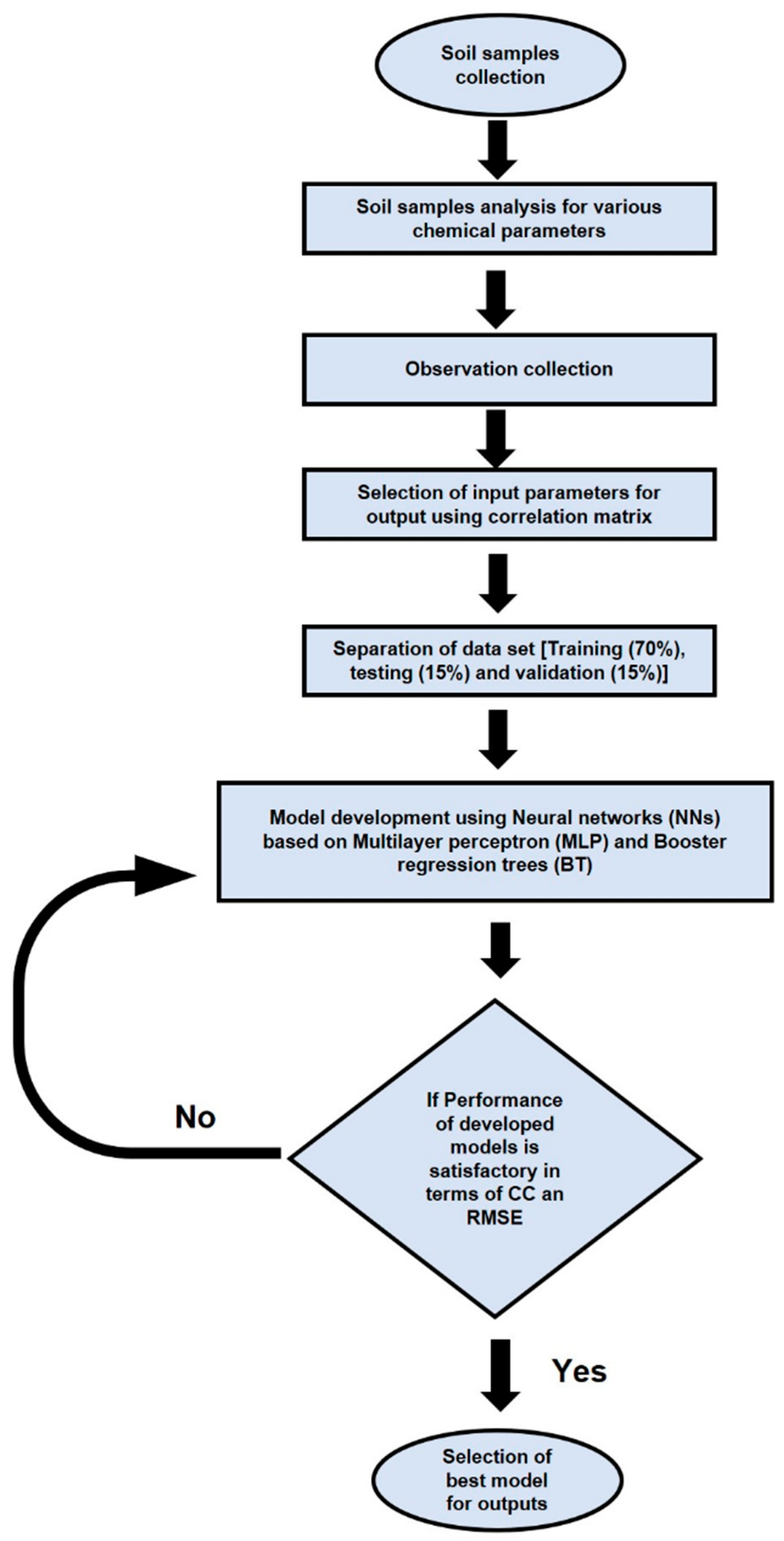
2. Materials and Methods

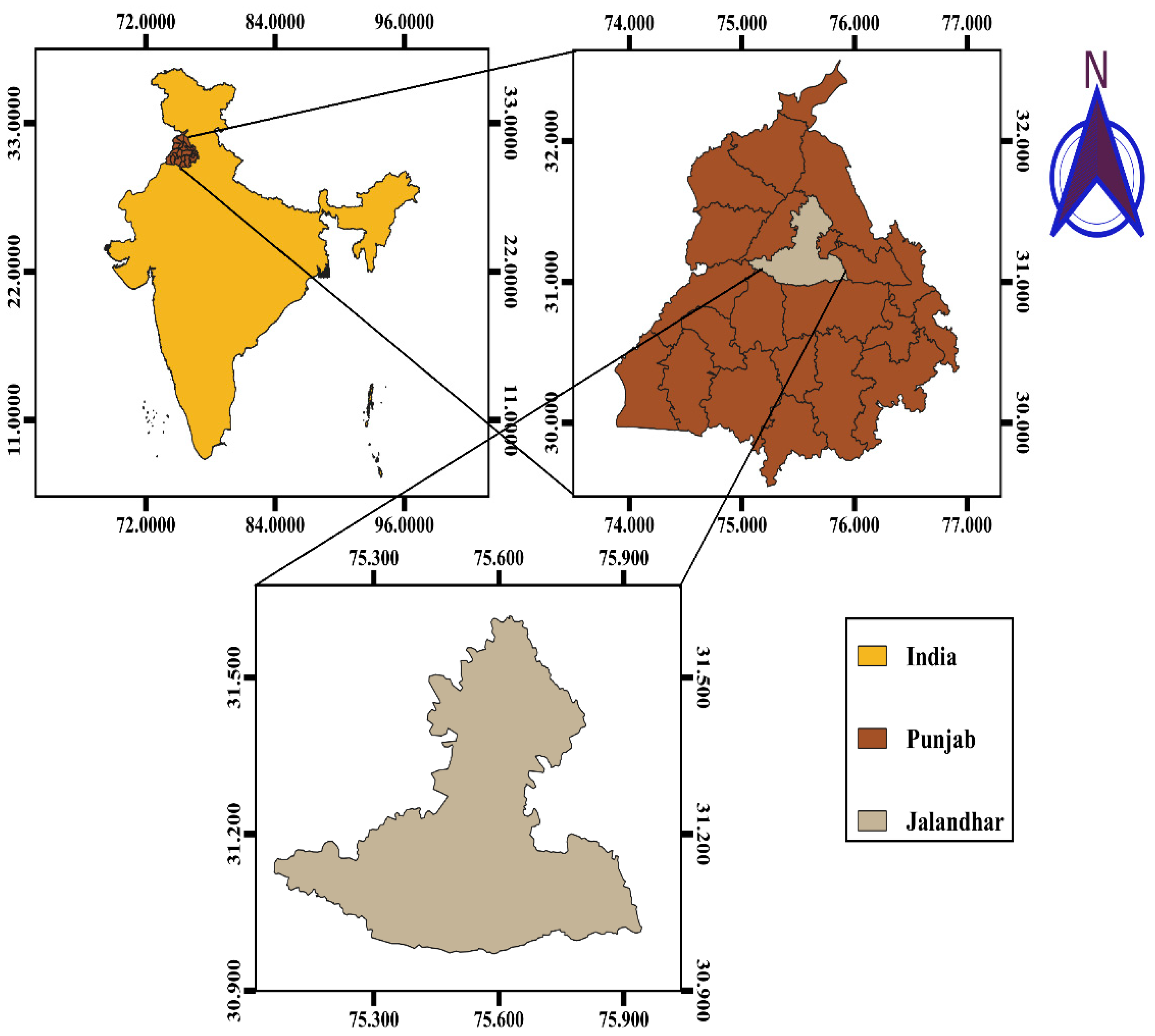
2.1. Study Area

The current area of assessment was District Jalandhar, Punjab. This District is located between two rivers; Beas and Sutlej. Loamy soil is mainly found in this area, which is due to the cool to warm climate based on sub-moist environments [34]. The geological substrate consists of alluvial deposits from the Quaternary age associated with 81 Indus allivial plains [35]. It makes up approximately 5.35% of the area of Punjab, and is one of the most highly populated areas of Punjab. The land consists of 90% agriculture, 7.4% non-agriculture and 2.1% forests. It has an extensive setup of roads and is a significant location for agriculture as well as textile and automobile spare part factories [32]. The climate of the study area is normally very hot during the summer season and very cold during the winter season, with rice and wheat as the main crops in the study area. The annual rainfall is about 600 mm year⁻¹. When samples were collected, the humidity was 77% and the temperature was 18 °C.

2.2. Soil Sampling and Analysis of Chemical Properties of Soil

Samples were collected at a depth of 0–15 cm from 70 locations in triplicates from Jalandhar (India) (Figure 1). Soil samples were air-dried and analyzed for various chemical parameters (pH, phosphorus (P), Ca, Mg, and organic carbon (C)) and PTEs (Co, Pb and Cu). Soil pH was measured by employing micro pH Analytical pH-meter in 1:2 soil/water extracts [36]. The Olsen method was applied to determine phosphorus [37], while calcium and magnesium were determined through EDTA titrations [38]. Walkley-Black wet oxidation method was used to determine C content [39]. The pseudototal Co, Cu and Pb contents were determined by acid digestion using aqua regia (HNO₃: HCl, 1:3 v/v). One gram of each oven-dried soil sample was digested with 12 mL of aqua regia and the solution was heated on the hot plate for 1–2 h. The digested samples were filtered and diluted with 50 mL of steam distillation water and used for analysis. Element analysis in the extracts was resolute by atomic absorption spectrophotometer (AAS) (Model Agilent Technologies 200-Series AA). The limits of detection of the instrument are as follows: 5 µg L⁻¹ for Co, 1.2 µg L⁻¹ for Cu and 14 µg L⁻¹ for Pb. More details are given in Kumar et al. [33].

2.3. Stepwise Regression for Input Selection

The set of factors used for input vectors were pH, P, Ca, Mg and C. The corresponding outputs were Co, Cu and Pb. We accepted that the input vectors encompassed features that are expedient for influencing the output of PTEs. Afterwards, the variable selection method, i.e., the stepwise regression analysis, in which various combinations of input variables were tested together for input selection and pH and P were selected based on higher R² and lower residual mean square in Analysis of Variance (ANOVA) regression. Before analysis, data pre-processing was implemented using Sigma Plot (v. 12.0) and outliers were separated and then data dropped to 67 for further modeling processes. Subsequently, the data points were divided by the randomization technique. Data points were randomized and spited by Microsoft Excel software, and 70% of the data was selected to train the models and remaining 30% was used to test (15%) and validation (15%) of the developed models.

2.4. Modeling Techniques

Modeling approaches such as neural networks (NNs) based upon multilayer perceptron (MLP) and boosted regression trees (BT) are used in this paper for modeling of PTEs. The boosted regression trees (BT) are a group of two techniques; boosted and decision tree. Boosted was implemented with traditional techniques such as decision tree, M5P, support vector machine, etc. to improve performance. The basic principle of artificial neural network is human brain. The principally used design of NNs is serened of input, output and hidden layers known as MLP [38,39,40,41]. The details vis à vis modeling approaches were given in Shiri et al. [42,43] and Sihag et al. [15].

2.5. Model Performance Assessing Parameters:

For appraising the guessing aptitude of diverse approaches, the coefficient of correlation (CC) and root mean square error (RMSE) values were enumerated by using training and testing statistics. Elaborations are provided in earlier research by Sihag et al. [15].

$$\mathrm{Coefficient}\mathrm{of}\mathrm{correlation}=\frac{n{\displaystyle \sum }{E}_{obs}{E}_{pred}–({\displaystyle \sum }{E}_{obs})({\displaystyle \sum }{E}_{pred})}{\sqrt{n({\displaystyle \sum }{E}_{obs}{}^2)-{({\displaystyle \sum }{E}_{obs})}^2}\sqrt{n({\displaystyle \sum }{E}_{pred}{}^2)-{({\displaystyle \sum }{E}_{pred})}^2}}$$

(1)

$$\mathrm{Root}\mathrm{mean}\mathrm{square}\mathrm{error}=\sqrt{\frac{1}{n}({\displaystyle \sum }_{i=1}^n{\left(E_{obs}-E_{pred}\right)}^2}$$

(2)

where: E_obs and E_pred are experiential and prophesied values, and n is number of observations. Figure 2 represents the overview of this paper.

3. Results and Discussion

The aim of the study was to evaluate the effectiveness of MLP- and BT-based models to predict the Co, Cu and Pb in the soil. Data used in this study were gathered from field data. Figure 3 shows the correlation matrix of the dataset. Phosphorus and pH are positively correlated with Cu, Co and Pb, while Ca negatively correlates with these metals. Mg showed a moderate correlation with Cu, Co and Pb. Organic carbon also exhibits a moderate negative relationship with these elements. Figure 4 indicates the 3D plot of pH and P versus Co, Cu and Pb, respectively, dependent upon a set of three-dimensional points. These plots depict the relationship of phosphorus and pH with concentrations of Cu, Co and Pb. The effect of absolute variable can be examined using distinct plotting colours for the individual value of each variable. With the increasing concentration of phosphorus, the Co content increases, while the relationship of pH with Co shows that the concentration enhances with increasing values of pH, and maximum increase takes place at a pH value of 7.0. The maximum increase in Cu concentration occurs at phosphorus content 0.10 (mg kg⁻¹) and pH value of 7.3, while in Pb, maximum enhancement occurs at 0.20 (mg kg⁻¹) value of phosphorus and 7.0 value pH. Correlation coefficient and RMSE were used to assess the performance of developed models. The dataset consisted of 67 observations of studied variables where we can observe high levels of available P, and low levels of studied PTEs (

Table 1. Descriptive statistics of studied variables (n = 67).

Variables	Units	Mean	Minimum	Median	Maximum	SD	CV	Skewness
pH		7.76	6.70	7.88	8.80	0.41	0.05	−0.21
C	%	3.66	1.78	3.51	6.70	0.99	0.27	0.80
P	mg kg−1	128.97	7.00	132.85	355.20	74.94	0.58	0.44
Ca	meq 100g−1	0.19	0.05	0.14	0.93	0.15	0.79	3.68
Mg	meq 100g−1	0.17	0.02	0.15	0.90	0.13	0.74	3.37
Co	mg kg−1	0.10	0.01	0.11	0.36	0.09	0.91	0.37
Cu	mg kg−1	0.51	0.01	0.19	12.79	1.99	3.89	5.77
Pb	mg kg−1	0.23	0.01	0.15	5.83	0.70	2.98	7.68

SD, Standard Deviation; C, Organic carbon; P, Available Phosphorus.

).

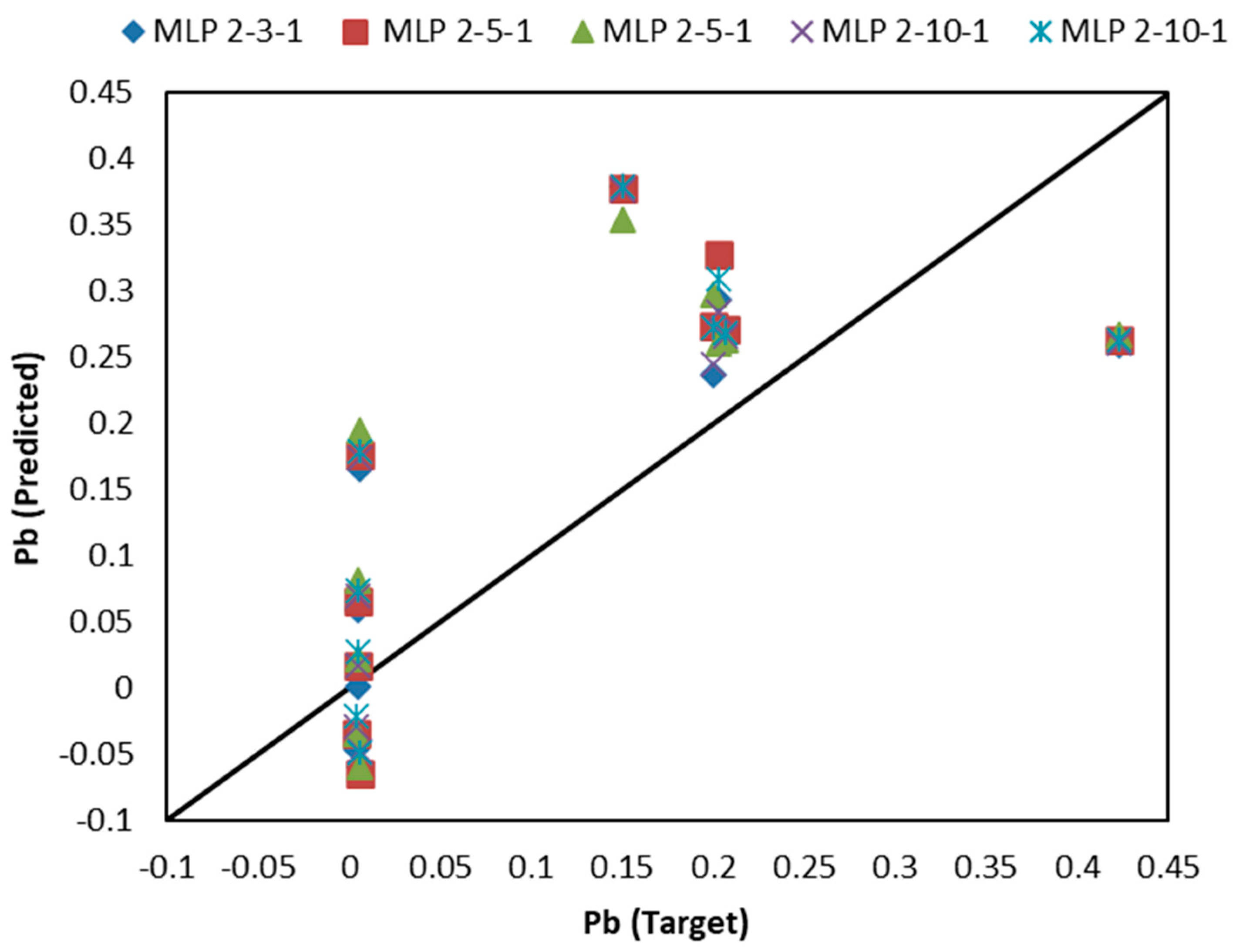
3.1. Results of MLP-Based Models

The neural network models based upon MLP were executed by employing MATLAB software. The selection of input variables is the initial step in soft computing-based models’ development. In this study, models were developed using pH, P, Ca, Mg and C variables. Model development is a trial-and-error process. A larger dataset was used for model preparation, and other (smaller) datasets were used for model testing and validation. Different input combinations were used to be developed for predicting the Co, Cu and Pb. After analyzing Pearson’s correlation matrix, five different models were developed. The different models are developed using a number of neurons in the hidden layer, and number of runs for output variables are Co, Cu and Pb. Figure 4 indicates the scatter plot of target and predicted values of Co using various MLP models. MLP-2-8-1 lies significantly closer to the line of perfect agreement (1:1) with lesser deviation. The model MLP-2-8-1 is best for predicting Co content, and the 2 signifies the number of input combinations (pH and phosphorus), while the 8 represents the number of neurons in a single hidden layer.

Table 2. Correlation coefficients and RMSE for different MLP topologies in all stages for Co.

Models		Training		Testing		Validation
	Run	CC	RMSE	CC	RMSE	CC	RMSE
MLP 2-8-1	10	0.8676	0.0453	0.7226	0.0416	0.4026	0.0082
MLP 2-5-1	10	0.8574	0.0469	0.7107	0.0162	0.4582	0.0070
MLP 2-5-1	25	0.9075	0.0383	0.7645	0.0148	0.3138	0.0125
MLP 2-8-1	25	0.8547	0.0474	0.7186	0.0193	0.5119	0.0060
MLP 2-6-1	25	0.8511	0.0479	0.6662	0.0144	0.4769	0.0070

indicates the values of coefficient of correlation and RMSE for all developed models for Co. Table 2 and Figure 5 suggest that that Model 4 that has the structure 2-8-1 is the best performing of all the developed models for all stages of model development with CC values in training (0.8547), testing (0.7186) and validation (0.5119), compared to the RMSE values obtained in training (0.0474), testing (0.0193) and validation (0.0060).

Figure 6 shows the scatter plot of target vs. output Cu using various models for the validation stage. MLP-2-10-1 lies closer to the line of perfect agreement (1:1), while deviation is much less.

Table 3. Correlation coefficient and RMSE values for different MLP topologies in all stages for Cu.

Models		Training		Testing		Validation
	Run	CC	RMSE	CC	RMSE	CC	RMSE
MLP 2-4-1	25	0.9407	0.0557	0.7420	0.0878	0.6635	0.1440
MLP 2-10-1	25	0.9488	0.0519	0.7366	0.0891	0.8626	0.0943
MLP 2-7-1	25	0.9331	0.0591	0.7554	0.0874	0.7883	0.0564
MLP 2-5-1	25	0.9372	0.0573	0.7264	0.0901	0.6828	0.0903
MLP 2-9-1	25	0.9463	0.0531	0.7393	0.0886	0.5610	0.0686

indicates the values of coefficient of correlation and RMSE for all developed models for Cu. This table suggests that Model 2, which has the structure 2-10-1 is the best performing of all the developed models for training and validation stages and shows comparable results in the testing stage with CC values in training (0.9488), testing (0.7366) and validation (0.8626), compared to the RMSE values obtained in training (0.0519), testing (0.0891) and validation (0.0943). The model MLP-2-10-1 is best for predicting the Cu concentration, and the 2 indicates the number of input variables used to build the model (pH and P) and the 10 indicated the number of neurons in a single hidden layer.

Figure 7 shows the scatter plot of target vs. output Pb using various models for the validation stage, and the MLP-2-10-1 model lies closer to the line of perfect agreement (1:1), while deviation is much less.

Table 4. Correlation coefficients and RMSE values for different MLP topologies in all stages for Pb.

Models		Training		Testing		Validation
	Run	CC	RMSE	CC	RMSE	CC	RMSE
MLP 2-3-1	25	0.8561	0.0938	0.3529	0.1078	0.7132	0.0128
MLP 2-5-1	25	0.8465	0.0104	0.3490	0.1084	0.7113	0.0142
MLP 2-5-1	10	0.8378	0.0243	0.3602	0.1052	0.7119	0.0129
MLP 2-10-1	25	0.8562	0.0231	0.3706	0.1071	0.7114	0.0126
MLP 2-10-1	10	0.8518	0.0066	0.3563	0.1079	0.7095	0.0137

indicates the values of coefficient of correlation and RMSE for all the developed models for Pb, and this table suggests that that Model 4 with the structure 2-10-1 is the best performing of all the developed models for the training and validation stages, and shows comparable results in the testing stage with CC values in training (0.8562), testing (0.3706) and validation (0.7114), compared to RMSE values obtained in training (0.0231), testing (0.1071) and validation (0.0126). The model MLP-2-10-1 is the best for predicting Pb content, and the 2 signifies the number of input combinations (pH and phosphorus) and 10 is the number of neurons in a single hidden layer. From the inferences obtained using MLP models, we can say that metals concentration may nearly be appraised with these neural network models and it is comparatively easy to assess variables; it can be promising to identify metals that are detrimental to the feasibility of soils, both rapidly and economically [44]. Scatter plots revealed that inferences obtained through MLP-based models of neural networks are acceptable for Cu, Co and Pb. Indeed, the determined models do not guarantee very high conformity amid assessments and amounts. However, this provides a useful method for assessing the eminence of soils [45]. El Badaoui [46], in their studies, applied a neural network approach based on MLP and multiple linear regression for predicting the concentration of Cu, Pb and Cr and inferred that NN models based on MLP are best predictors of the content of these metals with coefficients of determinations were 0.98 for Cu and 0.99 for Cr and Pb, respectively. Falamaki et al. [47] used various machine learning techniques in estimating the content of PTEs, for example, nickel, and concluded that our MLP-based NNs models better predict the content of PTEs in contrast with other models. Sihag et al. [15], while working on potentially toxic elements (Fe, Mn, Cu and Zn) in Neyshabur plain, Iran, applied different models such as NN-based MLP, M5 model tree (M5) and bagging approach (BM5P). They concluded that MLP models are the best predictors of Fe and Cu, while BM5P and M5P are appropriate models for predicting the Zn and Mn.

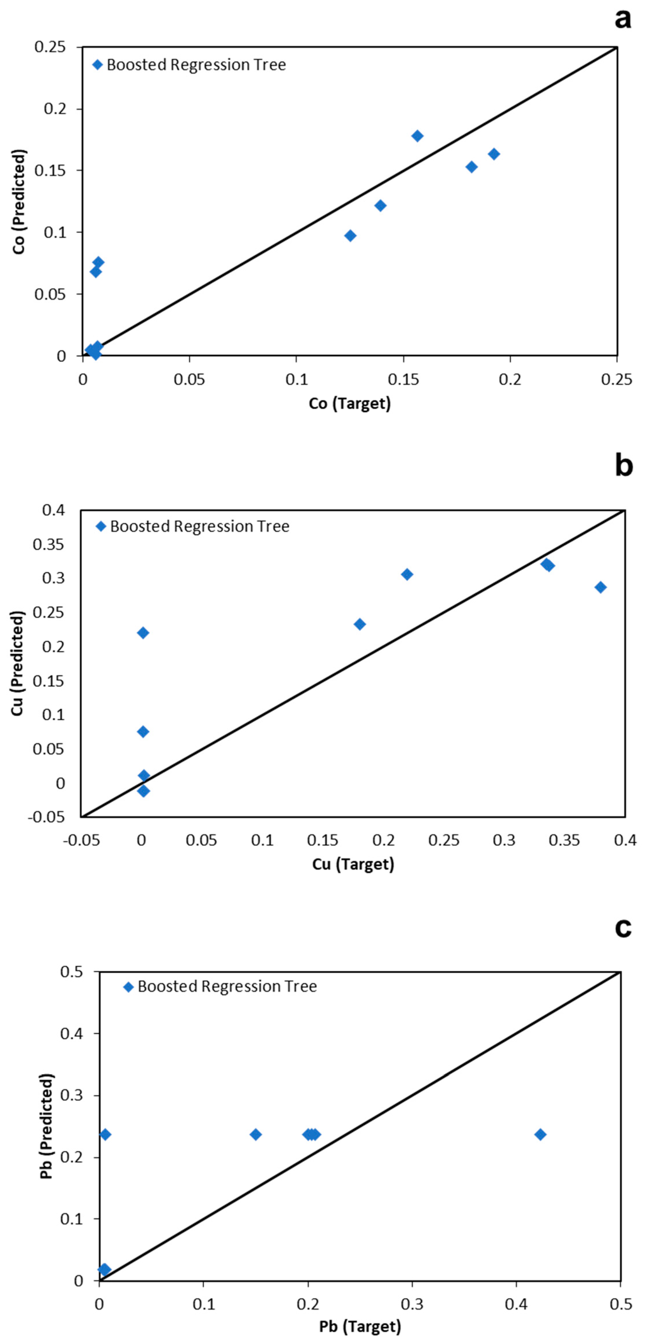
3.2. Results of BT-Based Models

Excerpt of input variables is the initial step in developing BT-based models. In the present paper, the model was established using pH, P, Ca, Mg, and C. Model development is a similar process as that followed by the MLP-based model development. Figure 8 indicates the BT model-based tree graphs for Co, Cu and Pb, respectively. The BT regression trees were obtained for Co, Cu and Pb using soil properties as forecasters. The root nodes of the regression tree in Co, spilt on phosphorus and pH, were also splitting variables into trees. It is assumed that lower phosphorus content is allied with greater Co retention, and pH is also an imperative variable in the retention of Co [48]. In the BT regression model of Cu and Pb, the root nodes of the regression tree also spilt on phosphorus and pH, and both these variables are imperative in maintaining Cu and Pb [49]. The agreement plots for target values and predicted values of Co, Cu and Pb are shown in Figure 9, respectively, using a validation dataset. CC and RMSE values of Co, Cu and Pb using BT-based models are listed in

Table 5. Correlation coefficients and RMSE values of Co, Cu and Pb using boosted regression tree method for all stages.

Output	Training		Testing		Validation
	CC	RMSE	CC	RMSE	CC	RMSE
Co	0.9159	0.0376	0.7092	0.0455	0.9062	0.0343
Cu	0.9600	0.0478	0.8646	0.0755	0.8539	0.0854
Pb	0.8000	0.1175	0.6450	0.0791	0.7064	0.1000

.

Among the predicted level of metals, the highest CC values were found for Cu in training (0.960) and testing (0.8646), while in the validation of models, the highest CC values were found for Co (0.9062). The RMSE values were recorded as the highest for Pb in training (0.1175), testing (0.0791) and validation (0.1000). Wei et al. [50] used boosted regression, random forest and support vector machine techniques for predicting the PTE concentration, mainly arsenic, and found that among all applied models, boosted regression is the best model for predicting the arsenic concentration with RMSE (0.6007). Hu et al. [51], in their studies for predicting the PTEs (Zn, Cu, Cr, Ni, Hg, Cd, As, and Pb) concentrations, applied numerous modelling techniques such as boosted regression, random forest and generalized linear models. Among the applied models, random forest is the best, followed by boosted regression and generalized linear models for predicting the concentration of these PTEs with RMSE values Zn (0.067), Cu (0.059), Cr (0.033), Ni (0.044), Hg (0.021), Cd (0.229), As (0.103) and Pb (0.004).

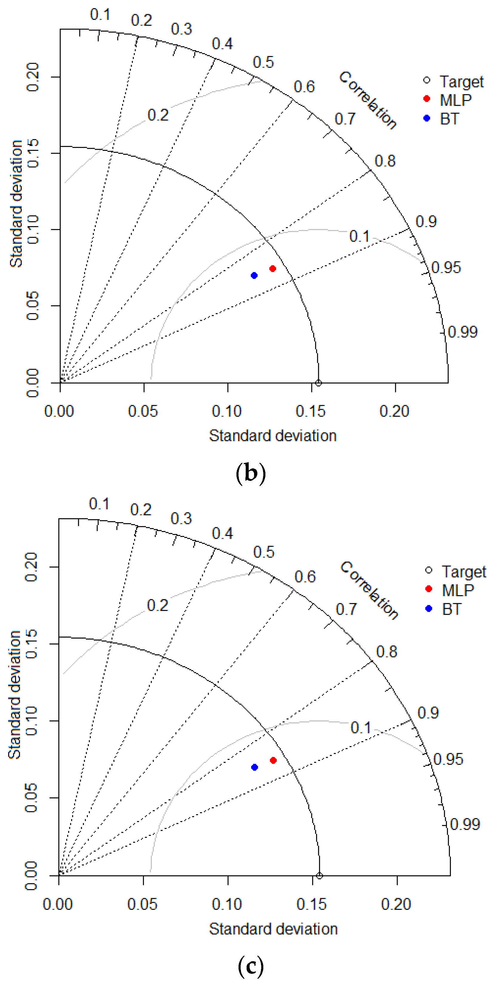
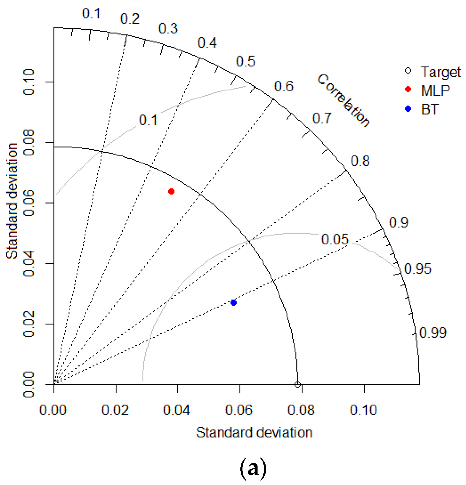
3.3. Intercomparison of Applied Models

To better elucidate the model prophecy impact further, we applied the Taylor diagram [52]. The nearer the pentagram was to this line, the nearer the prophecy was to determine the Cu, Co and Pb concentration prediction [53]. The Taylor diagram is a polar graph in which the cosine of the angle amid the X-axis is the CC in Cu, Co and Pb of the model. The radial direction is the ratio of model to metals standard deviation. The grey arcs signify the RMSE normalized by the standard deviation for the apiece model [54]. Figure 10 shows the Taylor diagram for the comparison coefficient of correlation and RMSE in the validation stage for predicting Co, Cu and Pb using applied models. This suggests that MLP-established models perform better than BT-built models for predicting the Cu and Pb, whereas BT models perform better than MLP-based models in predicting the Co. Overall, the neural network models based on MLP are closer to the line and fit well, in contrast with other models for predicting the concentration of Cu, Co and Pb.

4. Conclusions

The contamination by PTEs is a severe concern for soils worldwide, and proper attention should be paid to overcoming this problem. Proper mitigation approaches are needed, and this study concludes that the concentration of Cu, Co and Pb in roadside soils was found less in contrast with Indian soil limits. We tried to predict the level of these elements using modelling techniques. We found that amid all the applied techniques, we can conclude that MLP-based models perform better than BT-based models for predicting the Cu level with RMSE (0.0519 to 0.0943) and CC (0.5619 to 0.9488) and Pb level with RMSE (0.0066 to 0.1084) and CC (0.3490 to 0.8562), while BT models perform better than MLP-established models in predicting the Co levels with RMSE (0.0343 to 0.0455) and CC (0.7092 to 0.9159), respectively. Further BT-based regression models indicate that pH and phosphorus are the imperative variables in the retention of Cu, Co and Pb in the soil. These findings were supported by Pearson’s correlation analysis. Out of applied input soil variables in this study for model building, only phosphorus and pH exhibit a positive correlation with Cu, Co and Pb, and this may be why both these variables are imperative for the retention of Cu, Co and Co Pb in the soil of the studied region. The findings of the modelling techniques in the prophecy of Co, Cu and Pb helps ecological researchers to estimate the sites of effluence, causes and guidelines where the PTEs are disseminating. Planning appropriate environmental supremacy methods requires the mitigation of PTEs pollution in the environment. The present work provides significant information about the predicting power of machine learning techniques for Co, Cu and Pb concentration prediction and the models in which all datasets are grouped into a single learning framework. With the greater recitals and valuable characteristics of the generalized models, the projected scheme was effectively established for a set of Cu, Co and Pb; it should be executed further to a bigger dataset to form a widespread model.

References

1. Dogra, N.; Sharma, M.; Sharma, A.; Keshavarzi, A.; Minakshi, B.R.; Kumar, V. Pollution assessment and spatial distribution of roadside agricultural soils: A case study from India. Int. J. Environ. Res. Public Health 2020, 30, 146–159. [Google Scholar] [CrossRef] [PubMed]
2. Kumar, V.; Sharma, A.; Kaur, P.; Sidhu, G.P.S.; Bali, A.S.; Bhardwaj, R.; Cerda, A. Pollution assessment of heavy metals in soils of India and ecological risk assessment: A state-of-the-art. Chemosphere 2019, 216, 449–462. [Google Scholar] [CrossRef]
3. Rodrigo-Comino, J.; López-Vicente, M.; Kumar, V.; Rodríguez-Seijo, A.; Valkó, O.; Rojas, C.; Pourghasemi, H.R.; Salvati, L.; Bakr, N.; Vaudour, E.; et al. Soil science challenges in a new era: A transdisciplinary overview of relevant topics. Air Soil Water Res. 2020, 13, 1178622120977491. [Google Scholar] [CrossRef]
4. Panagos, P.; Van Liedekerke, M.; Yigini, Y.; Montanarella, L. Contaminated sites in Europe: Review of the current situation based on data collected through a European network. J. Environ. Public Health 2013, 2013, 158764. [Google Scholar] [CrossRef] [PubMed]
5. Kumar, V.; Sharma, A.; Kaur, P.; Kumar, R.; Keshavarzi, A.; Bhardwaj, R.; Thukral, A.K. Assessment of soil properties from catchment areas of Ravi and Beas rivers: A review. Geol. Ecol. Landsc. 2019, 3, 149–157. [Google Scholar] [CrossRef]
6. Keshavarzi, A.; Kumar, V. Spatial distribution and potential ecological risk assessment of heavy metals in agricultural soils of Northeastern, Iran. Geol. Ecol. Landsc. 2019, 4, 87–103. [Google Scholar] [CrossRef] [Green Version]
7. Harter, R.D.; Naidu, R. An assessment of environmental and solution parameter impact on trace-metal sorption by soils. Soil Sci. Soc. Am. J. 2001, 65, 597–612. [Google Scholar] [CrossRef]
8. Peakall, D.; Burger, J. Methodologies for assessing exposure to metals: Speciation, bioavailability of metals, and ecological host factors. Ecotox. Environ. Saf. 2003, 56, 110–121. [Google Scholar] [CrossRef]
9. Tóth, G.; Hermann, T.; Da Silva, M.R.; Montanarella, L. Heavy metals in agricultural soils of the European Union with implications for food safety. Environ. Int. 2016, 88, 299–309. [Google Scholar] [CrossRef] [PubMed]
10. Hou, D.; O’Connor, D.; Igalavithana, A.D.; Alessi, D.S.; Luo, J.; Tsang, D.C.W.; Sparks, D.L.; Yamauchi, Y.; Rinklebe, J.; Ok, Y.S. Metal contamination and bioremediation of agricultural soils for food safety and sustainability. Nat. Rev. Earth Environ. 2020, 1, 366–381. [Google Scholar] [CrossRef]
11. Keshavarzi, A.; Kumar, V. Ecological risk assessment and source apportionment of heavy metal contamination in agricultural soils of Northeastern Iran. Int. J. Environ. Health Res. 2019, 29, 544–560. [Google Scholar] [CrossRef] [PubMed]
12. Lin, Y.P.; Cheng, B.Y.; Shyu, G.S.; Chang, T.K. Combining a finite mixture distribution model with indicator kriging to delineate and map the spatial patterns of soil heavy metal pollution in Chunghua County, central Taiwan. Environ. Pollut. 2010, 158, 235–244. [Google Scholar] [CrossRef]
13. Rodríguez-Seijo, A.; Andrade, M.L.; Vega, F.A. Origin and spatial distribution of metals in urban soils. J. Soils Sediments 2017, 17, 1514–1526. [Google Scholar] [CrossRef]
14. Wang, Q.; Xie, Z.; Li, F. Using ensemble models to identify and apportion heavy metal pollution sources in agricultural soils on a local scale. Environ. Pollut. 2015, 206, 227–235. [Google Scholar] [CrossRef]
15. Sihag, P.; Keshavarzi, A.; Kumar, V. Comparison of different approaches for modelling of heavy metal estimations. SN Appl. Sci. 2019, 1, 780. [Google Scholar] [CrossRef] [Green Version]
16. Michel, K.; Roose, M.; Ludwig, B. Comparison of different approaches for modelling heavy metal transport in acidic soils. Geoderma 2007, 140, 207–214. [Google Scholar] [CrossRef]
17. Naderi, A.; Delavar, M.A.; Kaboudin, B.; Sadegh, A.M. Assessment of spatial distribution of soil heavy metals using ANN-GA, MSLR and satellite imagery. Environ. Monit. Assess. 2017, 189, 214. [Google Scholar] [CrossRef]
18. Ma, J.; Chen, Y.; Weng, L.; Peng, H.; Liao, Z.; Li, Y. Source Identification of Heavy Metals in Surface Paddy Soils Using Accumulated Elemental Ratios Coupled with MLR. Int. J. Environ. Res. Public Health 2021, 18, 2295. [Google Scholar] [CrossRef] [PubMed]
19. Toriz-Robles, N.; Ramírez-Guzmán, M.E.; Fernández-Ordoñez, Y.M.; Soria-Ruiz, J.; Ybarra, M. Comparison of linear and nonlinear models to estimate the risk of soil contamination. Agrociencia 2019, 53, 269–283. [Google Scholar]
20. Zhang, M.; Wang, X.; Liu, C.; Lu, J.; Qin, Y.; Mo, Y.; Xiao, P.; Liu, Y. Quantitative source identification and apportionment of heavy metals under two different land use types: Comparison of two receptor models APCS-MLR and PMF. Environ. Sci. Pollut. Res. 2020, 27, 42996–43010. [Google Scholar] [CrossRef]
21. Deng, M.H.; Zhu, Y.; Shao, K.; Zhang, Q.; Ye, G.H.; Shen, J. Metals source apportionment in farmland soil and the prediction of metal transfer in the soil-rice-human chain. J. Environ. Manag. 2020, 260, 110092. [Google Scholar] [CrossRef] [PubMed]
22. Gholami, R.; Kamkar-Rouhani, A.; Ardejani, F.D.; Maleki, S. Prediction of toxic metals concentration using artificial intelligence techniques. Appl. Water Sci. 2011, 1, 125–134. [Google Scholar] [CrossRef]
23. Sengorur, B.; Dogan, E.; Koklu, R.; Samandar, A. Dissolved oxygen estimation using artificial neural network for water quality control. Fresen. Environ. Bull. 2006, 15, 1064–1067. [Google Scholar]
24. Kuo, J.; Hsieh, M.; Lung, W.; She, N. Using artificial neural network for reservoir eutriphication prediction. Ecol. Model. 2007, 200, 171–177. [Google Scholar] [CrossRef]
25. Palani, S.; Liong, S.; Tkalich, P. An ANN application for water quality forecasting. Marin. Pollut. Bull. 2008, 56, 1586–1597. [Google Scholar] [CrossRef] [PubMed]
26. Hanbay, D.; Turkoglu, I.; Demir, Y. Prediction of wastewater treatment plant performance based on wavelet packet decomposition and neural networks. Expert. Syst. Appl. 2008, 34, 1038–1043. [Google Scholar] [CrossRef]
27. Singh, K.P.; Basant, A.; Malik, A.; Jain, G. Artificial neural network modeling of the river water quality—A case study. Ecol. Model. 2009, 220, 888–895. [Google Scholar] [CrossRef]
28. Chenard, J.F.; Caissie, D. Stream temperature modelling using neural networks: Application on Catamaran Brook, New Brunswick, Canada. Hydrol. Process. 2008, 22, 3361–3372. [Google Scholar] [CrossRef]
29. Dogan, E.; Sengorur, B.; Koklu, R. Modeling biochemical oxygen demand of the Melen River in Turkey using an artificial neural network technique. J. Environ. Manag. 2009, 90, 1229–1235. [Google Scholar] [CrossRef]
30. Chen, H.Y.; Yuan, X.Y.; Li, T.Y.; Sun, H.; Ji, J.F.; Wang, C. Characteristics of heavy metal transfer and their influencing factors in different soil–crop systems of the industrialization region, China. Ecotoxicol. Environ. Saf. 2016, 126, 193–201. [Google Scholar] [CrossRef]
31. Mu, T.; Wu, T.; Zhou, T.; Li, Z.; Ouyang, Y.; Jiang, J.; Zhou, D.; Hou, J.Y.; Wang, Z.Y.; Luo, Y.M.; et al. Geographical variation in arsenic, cadmium, and lead of soils and rice in the major rice producing regions of China. Sci. Total Environ. 2020, 677, 373–381. [Google Scholar] [CrossRef]
32. Kumar, V.; Kothiyal, N.C. Distribution behavior and carcinogenic level of some polycyclic aromatic hydrocarbons in roadside soil at major traffic intercepts within a developing city of India. Environ. Monit. Assess. 2012, 184, 6239–6252. [Google Scholar] [CrossRef] [PubMed]
33. Kumar, V.; Sharma, A.; Minakshi, B.R.; Thukral, A.K. Temporal distribution, source apportionment, and pollution assessment of metals in the sediments of Beas river, India. Hum. Ecol. Risk Assess. 2018, 24, 2162–2181. [Google Scholar] [CrossRef]
34. PSCST. Punjab State Council for Science & Technology, Chandigarh. Available online: http://punenvis.nic.in/index2.aspx?slid=205&mid=1&langid=1&sublinkid=62 (accessed on 21 February 2021).
35. Singh, A.; Sharma, C.S.; Jeyaseelan, A.T.; Chowdary, V.M. Spatio–temporal analysis of groundwater resources in Jalandhar district of Punjab state, India. Sustain. Water Resour. Manag. 2015, 1, 293–304. [Google Scholar]
36. Jackson, M.L. Soil Chemical Analysis; Prentice Hall of India. Pvt. Ltd.: New Delhi, India, 1967. [Google Scholar]
37. Olsen, S.R.; Cole, C.V.; Watanabe, F.S.; Dean, L.A. Estimation of Available Phosphorus by Extraction with Sodium Bicarbonate (Circular 39); USDA: Washington, DC, USA, 1954. [Google Scholar]
38. Tucker, B.B.; Kurtz, L.T. Calcium and Magnesium Determinations by EDTA Titrations. Soil. Sci. Soc. Am. J. 1961, 25, 27–29. [Google Scholar] [CrossRef]
39. Nelson, D.W.; Sommers, L.E. Total Carbon, Organic Carbon, and Organic Matter. In Methods of Soil Analysis; Page, A.L., Ed.; ASA and SSSA: Madisson, WI, USA, 1982; pp. 539–579. [Google Scholar]
40. Fausset, L.V. (Ed.) Fundamentals of Neural Networks: Architectures, Algorithms and Applications; Prentice Hall: Upper Saddle River, NJ, USA, 1994. [Google Scholar]
41. Park, Y.S.; Lek, S. Chapter 7-Artificial Neural Networks: Multilayer Perceptron for Ecological Modeling. In Developments in Environmental Modelling; Jørgensen, S.E., Ed.; Elsevier: Amsterdam, The Netherlands, 2016; Volume 28, pp. 123–140. [Google Scholar]
42. Shiri, J.; Keshavarzi, A.; Kisi, O.; Iturraran-Viveros, U.; Bagherzadeh, A.; Mousavi, R.; Karimi, S. Modeling soil cation exchange capacity using soil parameters. Comput. Electron. Agric. 2017, 135, 242–251. [Google Scholar] [CrossRef]
43. Shiri, J.; Keshavarzi, A.; Kisi, O.; Karimi, S.; Iturraran-Viveros, U. Modeling soil bulk density through a complete data scanning procedure: Heuristic alternatives. J. Hydrol. 2017, 549, 592–602. [Google Scholar] [CrossRef]
44. Ozel, H.U.; Gemici, B.T.; Gemici, E.; Ozel, H.B.; Cetin, M.; Sevik, H. Application of artificial neural networks to predict the heavy metal contamination in the Bartin River. Environ. Sci. Poll. Res. 2020, 27, 42495–42512. [Google Scholar] [CrossRef] [PubMed]
45. Bąk, Ł.; Szeląg, B.; Sałata, A.; Studziński, J. Modeling of Heavy Metal (Ni, Mn, Co, Zn, Cu, Pb, and Fe) and PAH Content in Stormwater Sediments Based on Weather and Physico-Geographical Characteristics of the Catchment-Data-Mining Approach. Water 2019, 11, 626. [Google Scholar] [CrossRef] [Green Version]
46. El Badaoui, H.; Abdallaoui, A.; Manssouri, I.; Lancelot, L. Application of the artificial neural networks of MLP type for the prediction of the levels of heavy metals in Moroccan aquatic sediments. Int. J. Comput. Eng. Res. 2013, 3, 75–81. [Google Scholar]
47. Falamaki, A. Artificial neural network application for predicting soil distribution coefficient of nickel. J. Environ. Radio. 2013, 115, 6–12. [Google Scholar] [CrossRef]
48. Covelo, E.F.; Matías, J.M.; Vega, F.A.; Reigosa, M.J.; Andrade, M.L. A tree regression analysis of factors determining the sorption and retention of heavy metals by soil. Geoderma 2008, 147, 75–85. [Google Scholar] [CrossRef]
49. Vega, F.A.; Matías, J.M.; Andrade, M.L.; Reigosa, M.J.; Covelo, E.F. Classification and regression trees (CARTs) for modelling the sorption and retention of heavy metals by soil. J. Hazard. Mater. 2009, 167, 615–624. [Google Scholar] [CrossRef] [PubMed]
50. Wei, L.; Yuan, Z.; Zhong, Y.; Yang, L.; Hu, X.; Zhang, Y. An improved gradient boosting regression tree estimation model for soil heavy metal (arsenic) pollution monitoring using hyperspectral remote sensing. Appl. Sci. 2019, 9, 1943. [Google Scholar] [CrossRef] [Green Version]
51. Hu, B.; Xue, J.; Zhou, Y.; Shao, S.; Fu, Z.; Li, Y.; Shi, Z. Modelling bioaccumulation of heavy metals in soil-crop ecosystems and identifying its controlling factors using machine learning. Environ. Pollut. 2020, 262, 114308. [Google Scholar] [CrossRef]
52. Guevara, M.; Olmedo, G.F.; Stell, E.; Yigini, Y.; Aguilar, D.Y.; Arellano, H.C.; Vargas, R. No silver bullet for digital soil mapping: Country-specific soil organic carbon estimates across Latin America. Soil 2018, 4, 173–193. [Google Scholar] [CrossRef] [Green Version]
53. Ge, X.; Wang, J.; Ding, J.; Cao, X.; Zhang, Z.; Liu, J.; Li, X. Combining UAV-based hyperspectral imagery and machine learning algorithms for soil moisture content monitoring. PeerJ 2019, 7, 6926. [Google Scholar] [CrossRef] [PubMed]
54. Wang, Z.; Liu, S.; Wang, Y.; Valbuena, R.; Wu, Y.; Kutia, M.; Shi, Y. Tighten the Bolts and Nuts on GPP Estimations from Sites to the Globe: An Assessment of Remote Sensing Based LUE Models and Supporting Data Fields. Remote Sens. 2021, 13, 168. [Google Scholar] [CrossRef]
Figure 1. Study area showing different sites.
Applsci 11 08362 g001
Figure 2. Flowchart of the work carried out in this paper.
Applsci 11 08362 g002
Figure 3. Correlation of input and target variables.
Applsci 11 08362 g003
Figure 4. 3D surface plot of Co (a), Cu (b) and Pb (c) versus pH and P showing a three-dimensional functional relationship between designated dependent variable (Z = Co, Cu and Pb) and two independent variables (X = pH, Y = P).
Applsci 11 08362 g004
Figure 5. Scatter plot of target vs. output Co using different neural networks models dependent on MLP in validation stage.
Applsci 11 08362 g005
Figure 6. Scatter plot of target vs. output Cu employing numerous neural network models based on MLP in validation stage.
Applsci 11 08362 g006
Figure 7. Scatter plot of target vs. predicted Pb using various neural networks models based upon MLP in validation stage.
Applsci 11 08362 g007
Figure 8. Boosted regression tree graph of Co (a), Cu (b) and Pb (c) (Mu, mean; Var, variance).
Applsci 11 08362 g008
Figure 9. Scatter plot of target vs. predicted Co (a), Cu (b) and Pb (c) using the boosted regression tree method in validation stage.
Applsci 11 08362 g009
Figure 10. Taylor diagram for Co (a), Cu (b) and Pb (c) based models. The colored dots epitomize the models in the corresponding legend.
Applsci 11 08362 g010aApplsci 11 08362 g010b