Article

Multi-Class Strategies for Joint Building Footprint and Road Detection in Remote Sensing

1
Tracasa Instrumental, Calle Cabárceno 6, 31621 Sarriguren, Spain
2
Institute of Smart Cities (ISC), Arrosadia Campus, Public University of Navarre (UPNA), 31006 Pamplona, Spain
*
Author to whom correspondence should be addressed.
Appl. Sci. 2021, 11(18), 8340; https://doi.org/10.3390/app11188340
Submission received: 22 July 2021 / Revised: 3 September 2021 / Accepted: 7 September 2021 / Published: 8 September 2021
(This article belongs to the Special Issue Computer Vision in the Era of Deep Learning)

Abstract

:
Building footprints and road networks are important inputs for a great deal of services. For instance, building maps are useful for urban planning, whereas road maps are essential for disaster response services. Traditionally, building and road maps are manually generated by remote sensing experts or land surveying, occasionally assisted by semi-automatic tools. In the last decade, deep learning-based approaches have demonstrated their capabilities to extract these elements automatically and accurately from remote sensing imagery. The building footprint and road network detection problem can be considered a multi-class semantic segmentation task, that is, a single model performs a pixel-wise classification on multiple classes, optimizing the overall performance. However, depending on the spatial resolution of the imagery used, both classes may coexist within the same pixel, drastically reducing their separability. In this regard, binary decomposition techniques, which have been widely studied in the machine learning literature, are proved useful for addressing multi-class problems. Accordingly, the multi-class problem can be split into multiple binary semantic segmentation sub-problems, specializing different models for each class. Nevertheless, in these cases, an aggregation step is required to obtain the final output labels. Additionally, other novel approaches, such as multi-task learning, may come in handy to further increase the performance of the binary semantic segmentation models. Since there is no certainty as to which strategy should be carried out to accurately tackle a multi-class remote sensing semantic segmentation problem, this paper performs an in-depth study to shed light on the issue. For this purpose, open-access Sentinel-1 and Sentinel-2 imagery (at 10 m) are considered for extracting buildings and roads, making use of the well-known U-Net convolutional neural network. It is worth stressing that building and road classes may coexist within the same pixel when working at such a low spatial resolution, setting a challenging problem scheme. Accordingly, a robust experimental study is developed to assess the benefits of the decomposition strategies and their combination with a multi-task learning scheme. The obtained results demonstrate that decomposing the considered multi-class remote sensing semantic segmentation problem into multiple binary ones using a One-vs.-All binary decomposition technique leads to better results than the standard direct multi-class approach. Additionally, the benefits of using a multi-task learning scheme for pushing the performance of binary segmentation models are also shown.

1. Introduction

Deep learning is a subfield of machine learning inspired by the structures and learning processes in the human brain. Deep learning models automatically extract features from large amounts of data, reducing human intervention. In recent years, deep learning has received a lot of attention in both scientific research and practical application [1,2]. Three main factors are responsible for this growing attention: the availability of large-scale datasets [3,4,5]; the increase in computational processing power, especially with graphics processing units (GPUs) [6,7,8]; and the appearance of several mathematical frameworks for deep learning [9,10,11].
The progress made in deep learning has had a direct impact on computer vision tasks, where convolutional neural networks (CNNs) have excelled. CNNs consist of a concatenation of convolutional and pooling layers that progressively extract higher-level features from images. Deep learning advancements have greatly improved pixel-labeling tasks, where the aim is to assign a label to each pixel in an image. Accordingly, novel deep learning strategies have outperformed well-established approaches for applications, such as medical imaging analysis [12] and autonomous driving [13]. Moreover, deep learning techniques have also proved successful in a wide range of remote sensing tasks [14,15], including the detection of building footprints [16,17] and road networks [18,19].
Road networks and building footprints are of great importance nowadays since a great deal of services rely on them to properly work. Traditionally, very high-resolution satellite imagery were used to detect buildings and roads. However, the costs of this imagery and the low revisit times hinder the update frequency. Therefore, the use of open data with a high revisit frequency is compulsory in order to make it feasible to keep maps updated on a global scale.
The European Space Agency (ESA) plays a key role in the monitoring of these elements, making high-resolution Earth observation data more accessible and thus, encouraging the application of deep learning techniques to remote sensing problems. Specifically, ESA is currently developing in partnership with the European Commission, seven Sentinel missions under the Copernicus Program [20]. Each mission is focused on a different aspect of the Earth, such as the oceans, lands, or atmosphere. Among these missions, we find Sentinel-1 (S1) and Sentinel-2 (S2) high-resolution satellites. The high revisit times provided by these satellites open a great deal of use cases, including disaster monitoring, urban planning, defense and intelligence and so on. Although their imagery is not usually considered to detect buildings and roads, due to their limited spatial resolution (10 m), their usage sets a challenging problem scheme.
Building and road detection tasks are usually addressed as pixel-wise labeling tasks, also known as semantic segmentation tasks. A semantic segmentation scenario with only two classes is known as a binary segmentation problem. The detection of building footprints [21] and the extraction of road networks [22] are examples of binary segmentation problems. However, in the remote sensing literature, it is common to combine multiple classes to build up more elaborated maps. A semantic segmentation problem involving more than two classes is known as a multi-class segmentation problem. A recurrent example of a multiclass segmentation problem is the land cover and land use classification [23], which includes the joint detection of building and roads [24].
Over time, different strategies to address these problems have been established. While problems with only two classes have been tackled using binary semantic segmentation models [21,22], problems with more than two classes have been approached with multi-class models [23,25]. Since the latter optimizes the overall performance, the accuracy highly depends on the separability of the classes. When working with remote sensing imagery, low spatial resolution images may magnify this problem. This is the case of S1 and S2, where multiple classes can coexist within the same pixel, due to its limited spatial resolution. There are ways of reducing the complexity of multi-class problems, such as employing binary decomposition strategies or multi-task schemes. Nevertheless, to the best of our knowledge, no previous research has been conducted to define the best way to accomplish a multi-class semantic segmentation problem.
Many proposals have been developed, aiming at undertaking classification problems with more than two classes with a divide and conquer strategy [26], that is, the multi-class problem is divided into multiple binary classification problems, which is also known as binary decomposition [27]. Considering that multi-class problems are more complex than binary ones, decomposition techniques are expected to reduce the number of classification errors [27,28]. On the other hand, there are some drawbacks; for example, especial care should be taken to combine the outputs of these binary classifiers in order to build up the multi-class prediction [29].
One-vs.-One (OVO) [30] and One-vs.-All (OVA) [31] are among the most common decomposition schemes. The former learns a model to discriminate between each pair of classes, whereas the latter learns a model to distinguish between a single class and the remaining ones. Galar et al. [29] compared both decomposition techniques in several multiclass problems and showed that OVO outperformed OVA in the framework tested. Moreover, decomposition techniques have been proved successful for developing multi-class support vector machines (SVMs), outperforming other multi-class SVMs approaches.
Over the last decade, multi-task learning has received a lot of attention and has been successfully applied across a wide range of machine learning applications, including computer vision [32]. When facing multiple tasks simultaneously, an acceptable performance can be achieved by tackling each task independently. However, this approach ignores a wealth of information that might come in handy to the model. Accordingly, by sharing representations (training signals) between related tasks, the model may generalize better to the main task [33]. Multi-task learning has been successfully applied to a wide range of remote sensing tasks including the detection of buildings footprints [34] and the extraction of road networks [35]. Moreover, this approach can also be used in combination with a decomposition strategy to further improve the model performance.
The aim of this work is to determine how a multi-class semantic segmentation problem, such as the extraction of building footprints and road networks from high-resolution satellite imagery, should be properly tackled. It must be noted the high complexity of this scenario, given the low separability of the classes, due to the limited spatial resolution. In this regard, the standard multi-class approach will be compared to the aforementioned decomposition techniques. For this purpose, a multi-temporal dataset composed of 26 Spanish cities and two time intervals is generated. The dataset is divided into training and testing sets, according to the machine learning principles [36]. To assess the performance of the different approaches, the F-score and Intersection over Union (IoU) metrics are considered. Experiments demonstrate that decomposing a multi-class semantic segmentation problem into a set of binary segmentation sub-problems using an OVA strategy reduces the number of misclassified pixels and, hence, improves the overall segmentation mapping. Moreover, the results also show that a multi-task learning scheme can effectively be used to further increase the performance of the decomposed binary models.
The rest of this paper is organized as follows. Section 2 sets the problem statement and describes different multi-class semantic segmentation decomposition approaches. Then, the experimental framework is presented in Section 3. Thereafter, the experimental study is carried out, and the results are discussed in Section 4. Finally, Section 5 concludes this work and we present some future research.

2. Methods

In this section, the problem statement is set (Section 2.1). Then, the direct approach to address multi-class semantic segmentation problems is recalled (Section 2.2). Thereafter, the different decomposition strategies employed in this work are described (Section 2.3 and Section 2.4). Finally, the multi-task learning scheme as a way of improving the performance of semantic segmentation models is presented (Section 2.5).

2.1. Problem Statement

The detection of building footprints and road networks in high-resolution satellite imagery is a difficult multi-class semantic segmentation problem where a model is learned to label each pixel into building, road or background classes. However, given the limited spatial resolution of S1 and S2 (10 m), multiple classes may coexist within the same pixel, drastically increasing the complexity since the separability of the classes is reduced. These difficulties were experienced in our previous work [24], which was focused on the extraction of buildings and roads from S1 and S2 imagery. Binary decomposition strategies, such as OVO and OVA, address multi-class problems learning multiple binary models. Nevertheless, it must be noted that that the outputs of this models must be aggregated to build up the final multi-class prediction.

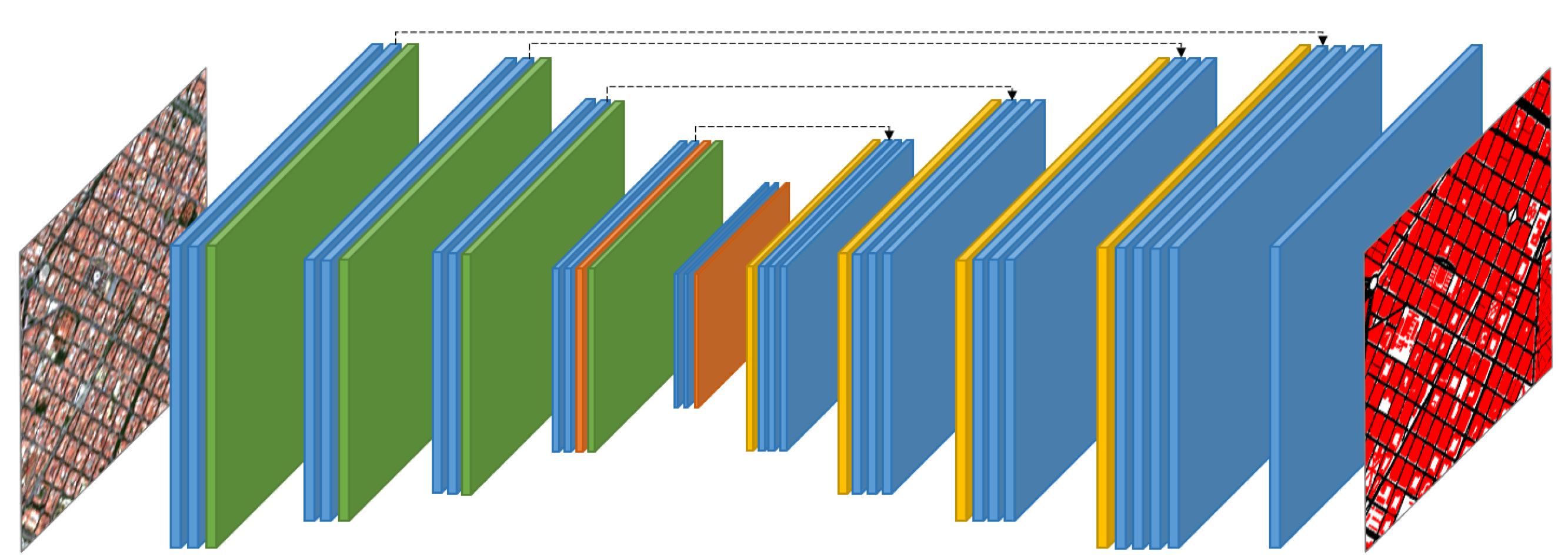
2.2. Direct Multi-Class Approach

A pixel-wise classification task involving more than two classes is known as a multi-class semantic segmentation problem. Here, the aim is to assign a label from a set of classes to each pixel on an image. However, depending on the use case, the boundaries between the classes may overlap, increasing the complexity of the pixel-labeling task.
The standard and most popular architecture for addressing semantic segmentation problems is the fully convolutional network (FCN), introduced by Long et al. [37]. The FCN was one of the first CNN-based architectures, where the segmentation map was obtained through a single forward pass. Moreover, since FCNs only have convolutional and pooling layers, they can make predictions on arbitrarily sized inputs. On the downside, multiple alternated convolutional and pooling layers downsample the resolution of the output feature maps, resulting in coarse object boundaries. However, novel semantic segmentation architectures based on the idea of FCNs, such as the SegNet [38], DeepLab [39] or U-Net [40], address this issue.
In this work, we have opted for the U-Net architecture, which has shown remarkable performance across a wide range of applications. As it is shown in Figure 1, this symmetric architecture consists of two major parts. The contracting path, also known as the encoder, reduces the spatial dimensions in every layer, while increasing the channel dimension. On the other hand, the expansive path, also known as the decoder, increases the spatial dimensions, while reducing the channel dimension. Both paths are symmetric and connected by the bottleneck. In the U-Net architecture, the feature maps extracted by the encoder are concatenated to the decoder, avoiding the loss of pattern information and thus, enabling precise localization.
The final 1 × 1 convolutional layer of the U-Net architecture performs the pixel-wise classification. Depending on the scenario, both the number of channels and the activation function employed in this layer may vary, that is, when addressing a binary semantic segmentation problem, the channel dimension will be set to 1, and the sigmoid will be used as the activation function. However, when facing multi-class settings, the channel dimension will be set to the total number of classes, and the softmax will be chosen as the activation function.

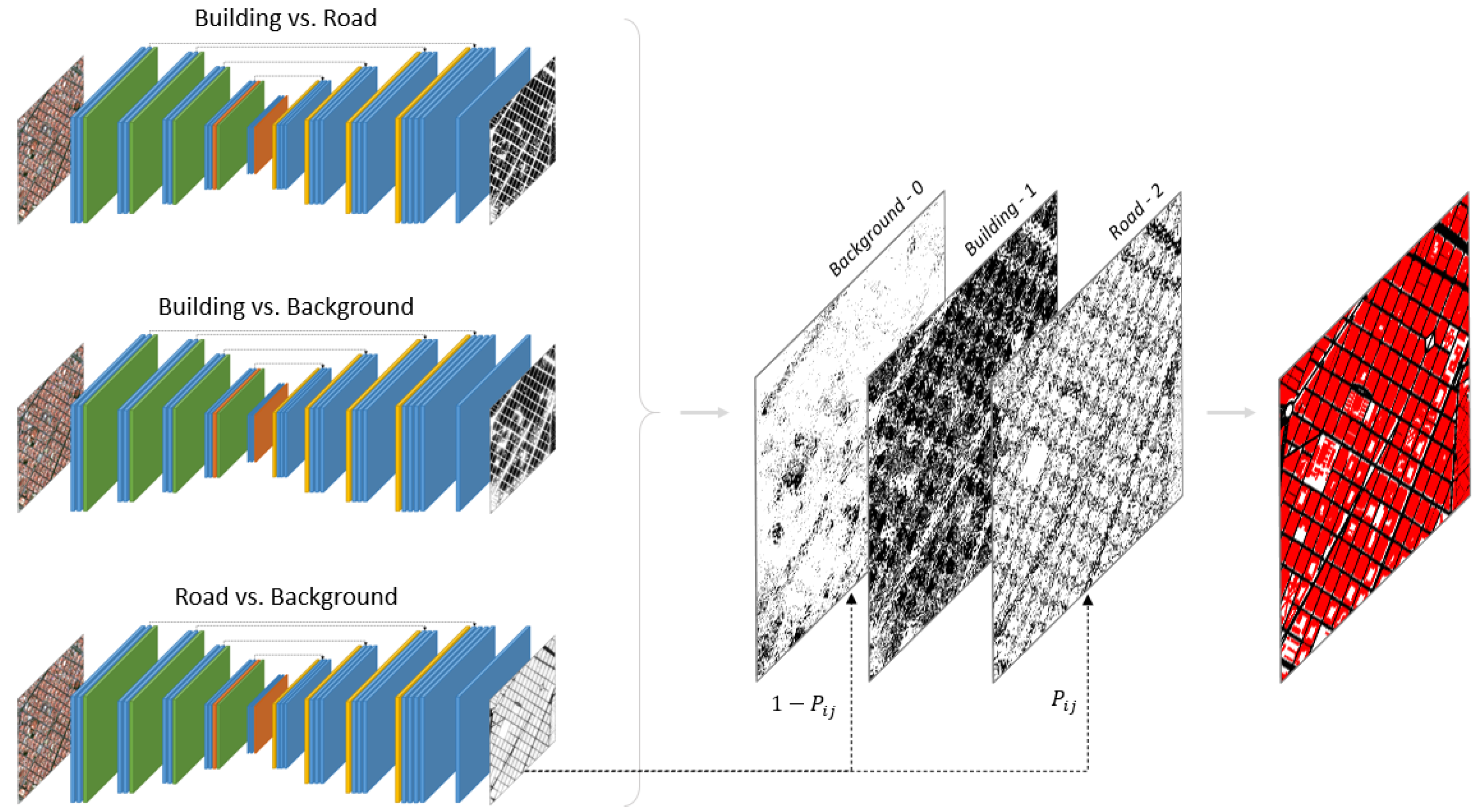
2.3. One-vs.-One Strategy

Multi-class semantic segmentation problems, like any other multi-class problem, can be decomposed into multiple binary semantic segmentation ones. OVO [30] is one of the most the most common strategies to decompose multi-class problems. Considering a scenario with N classes, the OVO decomposition scheme divides it into N ( N 1 ) / 2 binary sub-problems. At training time, only those pixels corresponding to one of the two discriminated classes are taken into account, ignoring the rest. Accordingly, pixels corresponding to ignored classes do not impact the loss function (but are considered for convolutions). In this work, given the problem statement, three binary models are learned: building-vs.-road, building-vs.-background, and road-vs.-background, as shown in Figure 2.
Although we have decomposed a complex multi-class problem into a priori multiple easier binary ones, drawbacks exist. For each pixel in the image, the outputs of the binary models must be aggregated to build up the multi-class prediction. To simplify the notation, for a given pixel, we use P i j to denote the confidence of the binary semantic segmentation model discriminating classes i and j in favor of the former one. As shown in Figure 2, each binary model contributes to the confidence of the positive class (i) with P i j and to the confidence of the negative class (j) with 1 P i j . To finally aggregate these confidence values, the weighted voting approach [41] is considered, that is, the class with the largest sum of confidence values is predicted in each pixel.

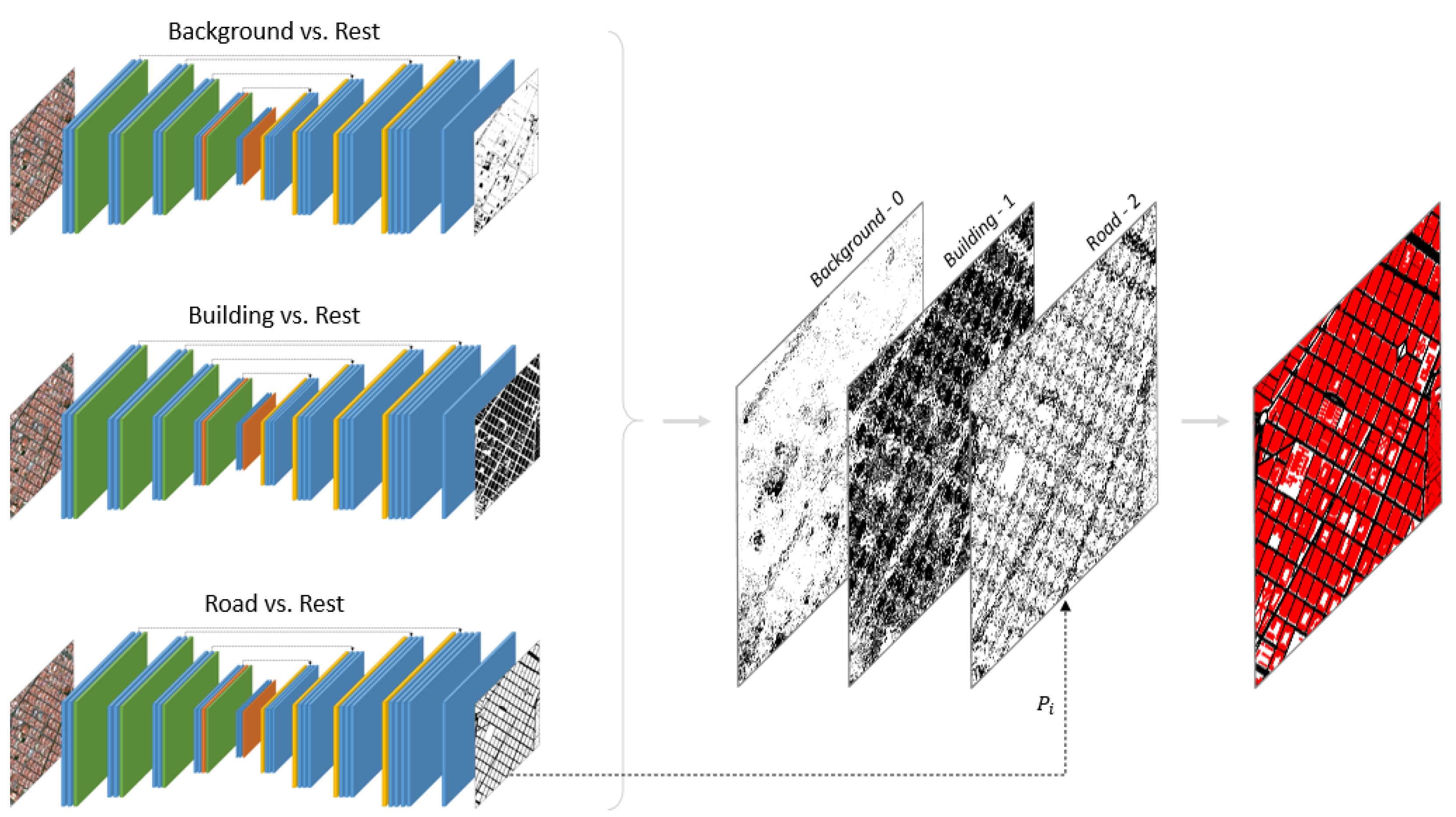
2.4. One-vs.-All Strategy

The OVA [31] decomposition scheme, like OVO, can be used to divide a multi-class semantic segmentation problem into multiple binary ones. Considering a scenario with N classes, the OVA strategy divides it into N binary sub-problems. In this strategy, each model is trained to discriminate between one class and the remaining ones. In this regard, it is common to have several more negative samples than positive ones, resulting in a highly imbalanced binary dataset. In this work, given the problem statement, three binary models are learned to detect buildings, roads and the background, respectively, as shown in Figure 3.
Again, the outputs of the binary models must be aggregated to generate the multi-class prediction. To simplify notation, we will use P i to denote the confidence of the binary semantic segmentation model discriminating the class i from the rest of classes for a given pixel. Accordingly, as Figure 3 depicts, each binary model contributes to the confidence of the positive class (i) with P i . Unlike OVO, the confidence in favor of the negative class is no longer used since each class is covered by a different model. To finally aggregate these values, the maximum confidence strategy [42] is used, that is, the class with the largest confidence is predicted.

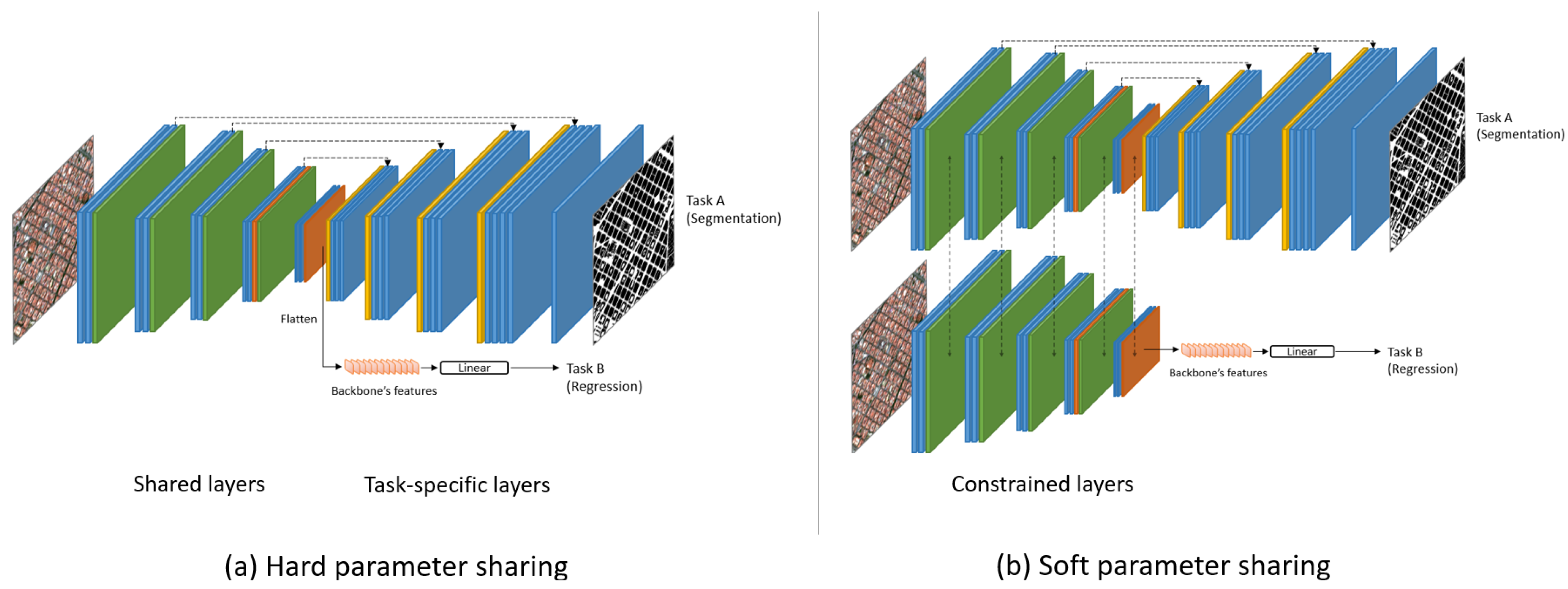
2.5. Multi-Task Strategy

Briefly, multi-task learning [33] consists of solving multiple learning tasks at the same time, exploiting commonalities and differences across them. Multi-task architectures are usually classified depending on how the parameters of the hidden layers are shared, as shown in Figure 4, where two tasks are considered (semantic segmentation and pixel count). In hard parameter sharing [43] (Figure 4a), the hidden layers between all tasks are shared, keeping some task-specific output layers. Being the most commonly used type of multi-task architecture, this approach greatly reduces the risk of overfitting since there are several tasks that are learned simultaneously, and the model has to find a representation that captures all of them. In soft parameter sharing [44] (Figure 4b), there are as many models as tasks, each one with its own parameters. It must be noted that the distance between these parameters is regularized to avoid overfitting.
In this work, we have opted for using the hard parameter sharing approach, considering that the soft parameter sharing one demands more resources and thus, becomes unfeasible when dealing with many classes. To further improve the performance of semantic segmentation models, the simplest complementary task is the prediction of the percentage of pixels assigned to each class. Therefore, Section 4 studies the application of this strategy to increase the performance of the base models. Figure 4 describes how this strategy is implemented. Accordingly, the features extracted by the encoder are passed through a linear layer that outputs the percentage of pixels assigned to the positive class.

3. Experimental Framework
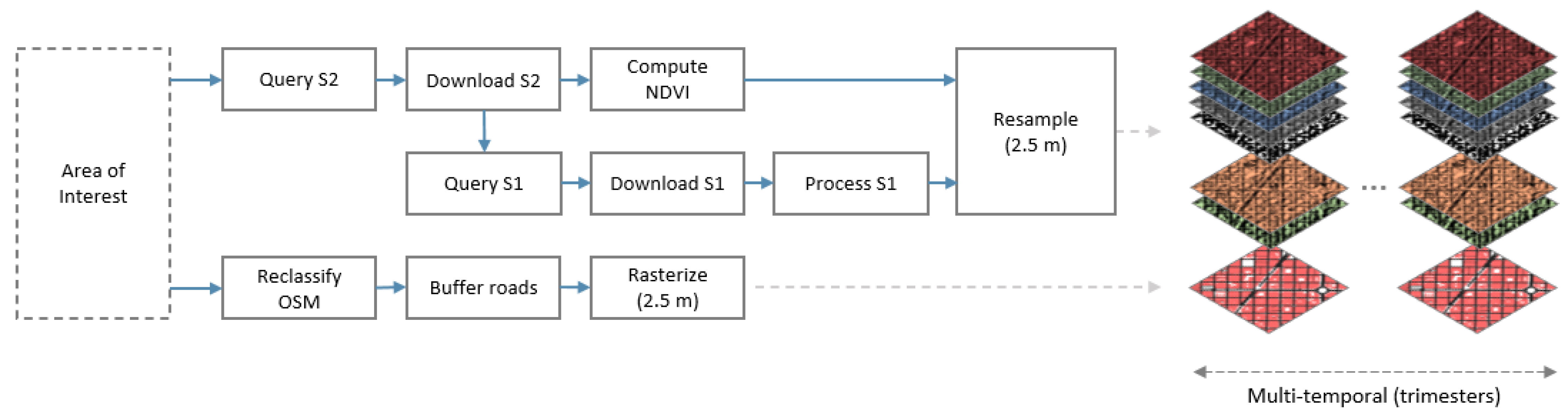
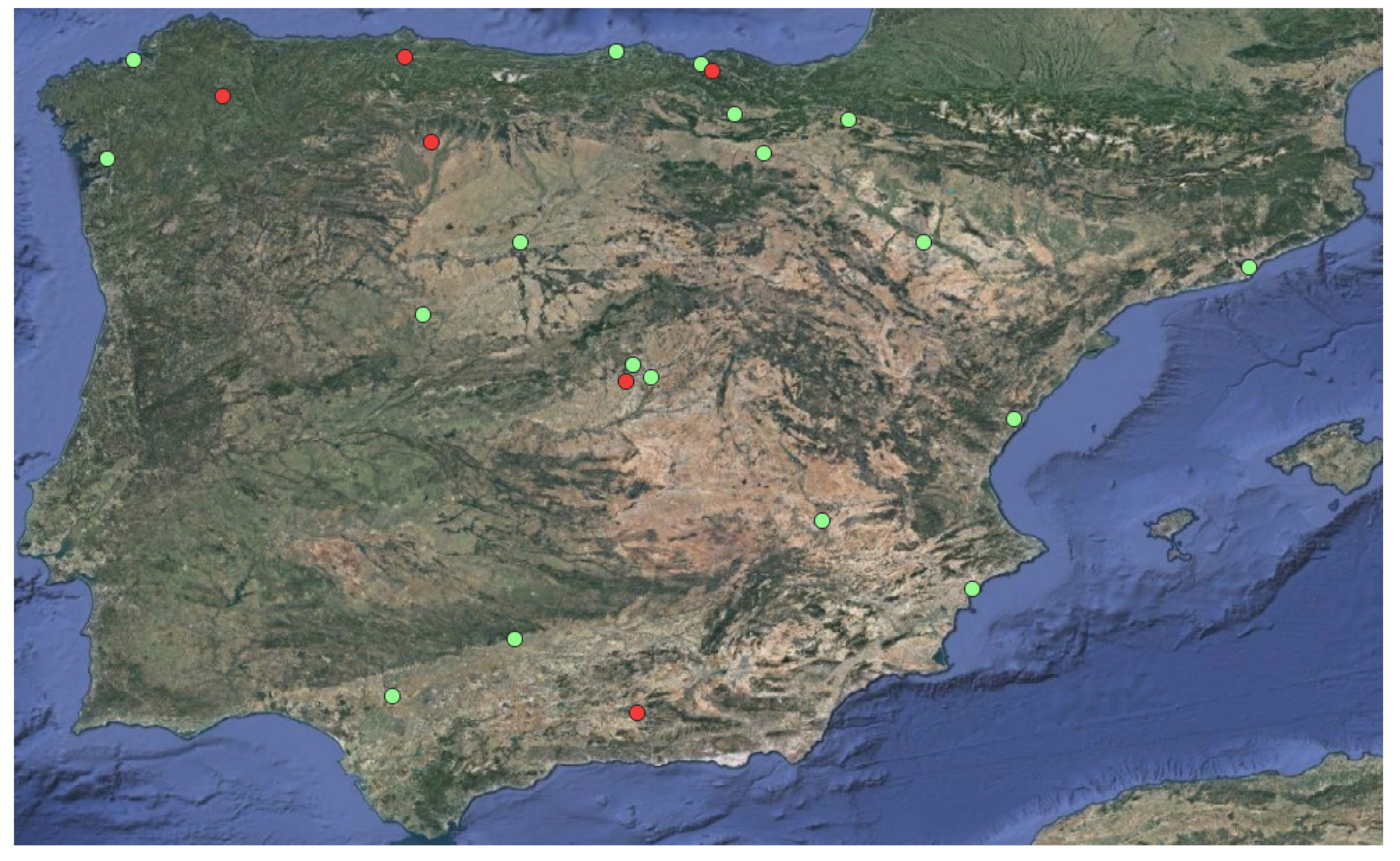
In this section, the experimental framework considered for carrying out the experiments is described. The dataset used across all the experiments is presented in Section 3.1. Then, the training procedure is detailed in Section 3.2. Finally, Section 3.3 explains the performance measures used to evaluate the different methods.

3.1. Dataset

In this work, we have opted for extracting buildings and roads from S1 and S2 imagery, given its limited spatial resolution (10 m). The lack of resolution reduces the separability of the building and road classes, increasing the multi-class problem complexity. In this way, the different approaches can be evaluated in a challenging problem. Accordingly, such a challenging scheme is required to properly evaluate the different approaches.
There are a great deal of remote sensing semantic segmentation datasets available. However, the vast majority of them consist of hand-labeled aerial imagery [45,46], which do not meet our requirements (road and building detection fusing S1 and S2 imagery). Despite the lack of high-resolution satellite imagery datasets, there are freely available geodatabases that can be used to generate ground truth masks for training deep learning models. Therefore, in this work, we have followed the methodology described by Ayala et al. [24]. Accordingly, we have used OpenStreetMap’s (OSM) [47] building and road labels, in combination with S1 and S2 to generate training and testing areas. It must be noted that OSM may contain labeling errors, especially in disseminated areas. Nevertheless, previous works [48] have demonstrated that when using large datasets, it is possible to reach a good performance, even if their labels are not accurate.
The dataset comprises several areas of interest. For a generic area of interest, the generation pipeline is illustrated in Figure 5. Given a bounding box and a time interval, S2 products are queried and downloaded from the Sentinels Scientific Data Hub (SciHub) [49]. It must be noted that only S2 products with less than a 5% cloud cover percentage are considered. In this work, we have opted for using the Red, Green, Blue and Near Infrared bands since they are the only ones provided at the greatest resolution of 10 m. Moreover, the Normalized Difference Vegetation Index (NDVI) is computed. To complement the optical information provided by S2, S1 VV and VH backscattering coefficients (in decibels) are downloaded from the SciHub and pre-processed, following the recommendations in [50]. Finally, S1 and S2 bands are stacked to create the 7-band inputs. In order to give models more room to detect hardly-visible buildings and roads, the 7-band inputs are resampled to 2.5 m.
As we have mentioned, the corresponding ground truth mask for the area of interest is generated, using OSM. Firstly, a reclassification is performed, aggregating geometries from different OSM classes, depending on the desired legend. Since in this work, we have focused on the detection of building and roads, several road types (OSM codes 5111-5115, 5121-5124 and 5132-5134) are fused into the road label, whereas building polygon silhouettes (OSM code 1500) are used for generating the building label. It must be noted that, since roads come as line-strings, they must be buffered prior to being rasterized. Finally, geometries are rasterized to 2.5 m in order to match the 7-band inputs spatial resolution.
In total, the final dataset is composed of 24 Spanish cities. These cities are divided into two sets, according to the machine learning guidelines [36]. With respect to the validation set, we have opted, after preliminary experiments, for not using this set. Hence, no early stopping is considered. Moreover, taking advantage of the high revisit times provided by both S1 and S2 satellites, two time-steps are considered for each city (December 2018–March 2019 and March 2019–June 2019). This approach allows one to not only improve the generalization capabilities of the models against color spectrum variations, but also to better assess the performance of the models in different time steps. Even though two trimesters are used in this work, this approach can be extrapolated to any number of trimesters, giving rise to more robust models and making their evaluation fairer. Moreover, shorter time intervals, such as months or weeks, can be used instead of trimesters.
The summary of the dataset is presented in Table 1. Recall that the training and testing split is done in such a way that prevents data leakage. That is, each city is assigned to a single set (either training or testing). Moreover, the testing set is manually inspected, invalidating areas where the labeling of OSM is not accurate. This allows us to make a fair evaluation of the models, considering only properly labeled areas. The remaining extension percentage after invalidation is also included for the testing set. The geographical distribution of the dataset within the Spanish territory is shown in Figure 6.

3.2. Training Details

All the models are trained for 100,000 iterations using the Adam [51] optimizer with a fixed learning rate of 1 × 10 3 . A batch size of 14 is used, considering the maximum number of samples that fits into memory. The experiments are run on a NVIDIA RTX 2080Ti with 11 GB of RAM.
Regarding the loss function, a combination of the cross-entropy and dice loss is considered. This approach, known as combo loss, is widely used in the remote sensing semantic segmentation literature [52]. In summary, the cross-entropy is used for curve smoothing, while the dice loss is used to control the trade-off between false positives and false negatives. These losses are computed as follows. Let C denote the set of all classes and I the set of pixels in an image. The cross-entropy and dice loss functions expressed in terms of the ground truth one-hot encoded mask y and the output probabilities y ^ are presented in Equations (1) and (2), respectively.
L C E ( y , y ^ ) = c C i I y i , c log ( y ^ i , c )
L D L ( y , y ^ ) = 2 i I c C y i , c y ^ i , c + 1 c C i I y i , c + y ^ i , c + 1
Considering that no validation set is used, the last epoch’s model is taken as the final model. To prevent overfitting [53] the dihedral data augmentation technique is used, that is, the data are augmented by applying horizontal and vertical flips, as well as 90 degree rotations, giving rise to 8 different combinations. The same data augmentation techniques are used at testing time. Accordingly, the final prediction is obtained as the aggregation of predictions across transformed versions of a test input.

3.3. Performance Measures and Evaluation

To evaluate the performance of the different approaches, the Intersection over Union (IoU) and F-score metrics are used (Equation (3)). Metrics are computed for each label (background, building and road) individually. Additionally, these metrics are aggregated over the different testing cities to assess the overall performance. This aggregation is done, using the weighted arithmetic mean, taking as weights the valid extension of each city. Recall that this information is presented in Table 1. Note that in Equation (3), both y and y ^ are one-hot encoded masks.
I o U ( y , y ^ , c ) = i I y i , c y ^ i , c i I max ( y i , c , y ^ i , c ) F s c o r e ( y , y ^ , c ) = 2 i I y i , c y ^ i , c i I y i , c + y ^ i , c
The performance of the different strategies is also qualitatively evaluated through the visual inspection of the multi-class segmentation maps. Additionally, the visual inspection of each label’s IoU in the form of true positives (TP), false positives (FP), true negatives (TN) and false negatives (FN) is also included. This outlook yields a better description of how the models are behaving, clearly identifying their differences.

4. Experimental Study

This section provides empirical evidence regarding how a multi-class segmentation problem in which buildings and roads are extracted from high-resolution satellite imagery should be adequately tackled. For this purpose, the following key questions are answered through individual experiments:
  • Can binary decomposition strategies be beneficial to address remote sensing multi-class semantic segmentation problems?
  • Can a multi-task learning scheme be used to further improve the performance in remote sensing semantic segmentation problems?

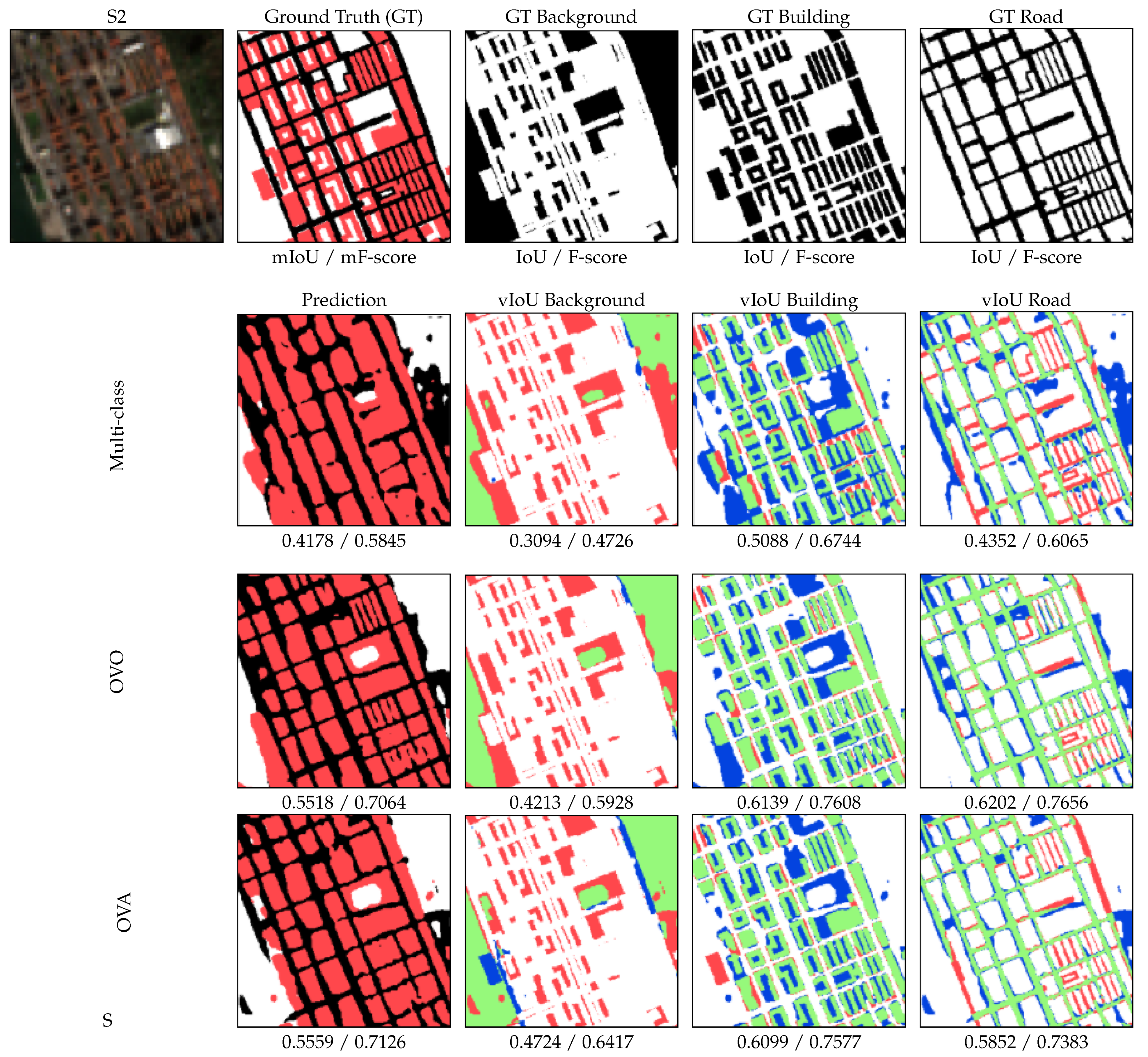
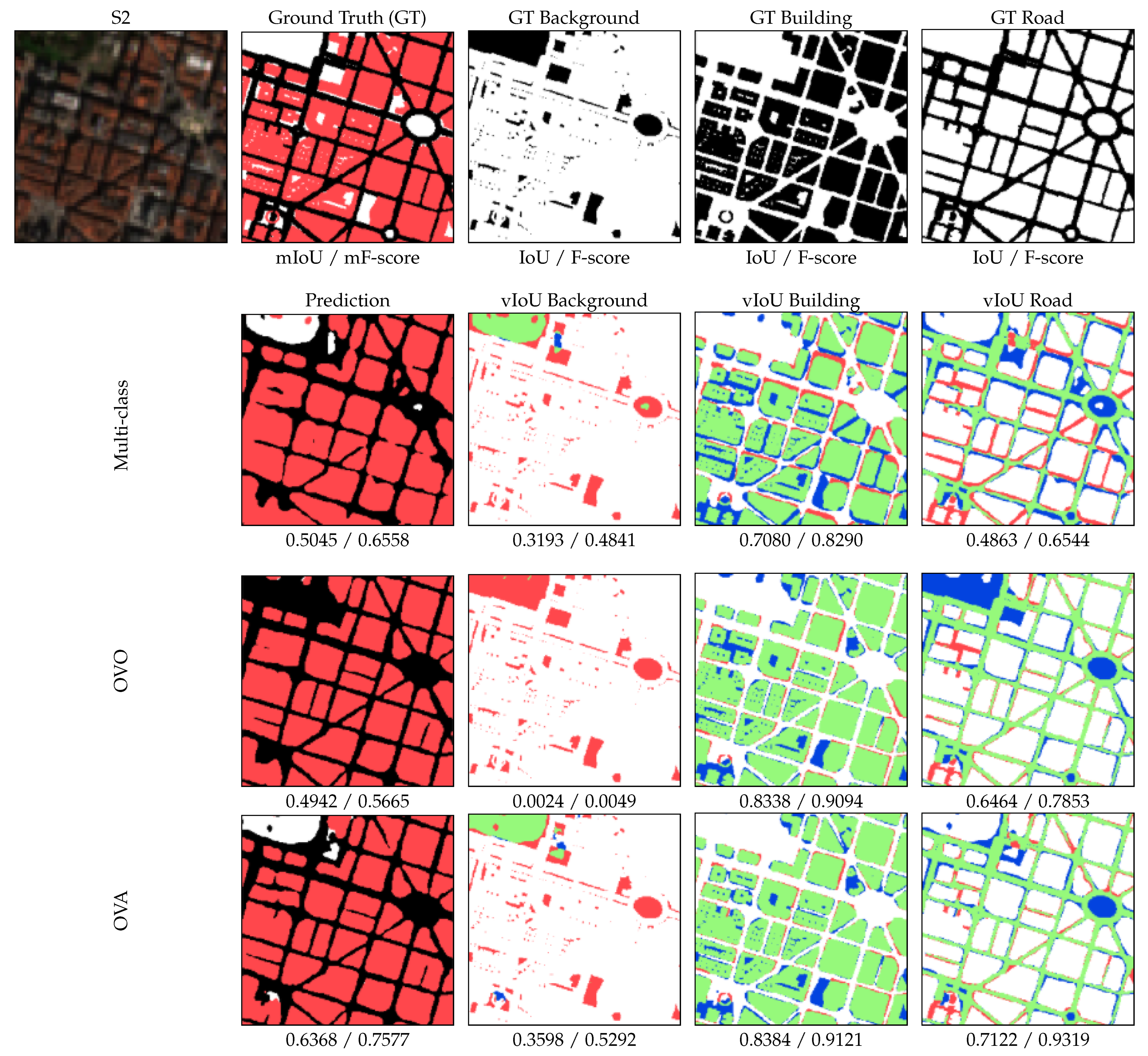
4.1. Experiment 1: Decomposing a Multi-Class Problem

In this experiment, OVO and OVA binary decomposition strategies are considered and compared to the standard multi-class semantic segmentation approach. Table 2 presents the results obtained in terms of the IoU and F-score not only for each label, but also for each city in the testing set. Additionally, the averaged metrics across the testing cities are also included. The best results achieved for each metric are presented in boldface.
The results show that decomposing a multi-class problem is an effective way to reduce the impact that the separability of the classes has on the overall performance. On the one hand, the OVO decomposition strategy increases the metrics from 0.6320, 0.3994 and 0.3565 to 0.8279, 0.5629 and 0.5427, in terms of averaged IoU, and from 0.7742, 0.5666 and 0.5252 to 0.9057, 0.7193 and 0.7021, in terms of averaged F-score, for each class (background, building and road), respectively. On the other hand, the OVA decomposition strategy increases the metrics from 0.6320, 0.3994 and 0.3565 to 0.8670, 0.5789 and 0.5828, in terms of averaged IoU, and from 0.7742, 0.5666 and 0.5252 to 0.9287, 0.7325 and 0.7347, in terms of averaged F-score, for each class (background, building and road), respectively.
Moreover, the OVA decomposition strategy leads to better results than the OVO (0.8670, 0.5789 and 0.5828 vs. 0.8279, 5629 and 0.5427, in terms of averaged IoU, and 0.9287, 0.7325 and 7347 vs. 0.9057, 0.7193 and 0.7093, in terms of averaged F-score, for each class (background, building and road), respectively). It must be noted that the OVO decomposition strategy achieves higher metrics in the building class for the Granada city than OVA (0.5745 vs. 0.5660 and 0.7297 vs. 0.7228, in terms of averaged IoU and F-score, respectively).
The quantitative results can be complemented with the qualitative results presented in Figure 7 and Figure 8. Here, the different approaches are contrasted, not only comparing their multi-class predictions but also through visual inspection of the IoU (vIoU) for each class in terms of true positives (TP) in green, false positives (FP) in blue, true negatives (TN) in white, and false negatives (FN) in red. Additionally, the averaged IoU and F-score metrics have been included.
A great deal of false positives (FP) can be observed in the final multi-class prediction for the direct multi-class approach. This is due to the limited spatial resolution since building and road classes may coexist within the same pixel. Accordingly, the direct multi-class approach optimizes the overall performance, choosing between both classes on detriment of the not selected one. However, as can be seen in the multi-class predictions generated by the OVO and OVA decomposition strategies, this issue is addressed. Even though OVO and OVA strategies perform similarly for the building class, it must be noted a major decrease in the false positives for the road class when using the latter one.

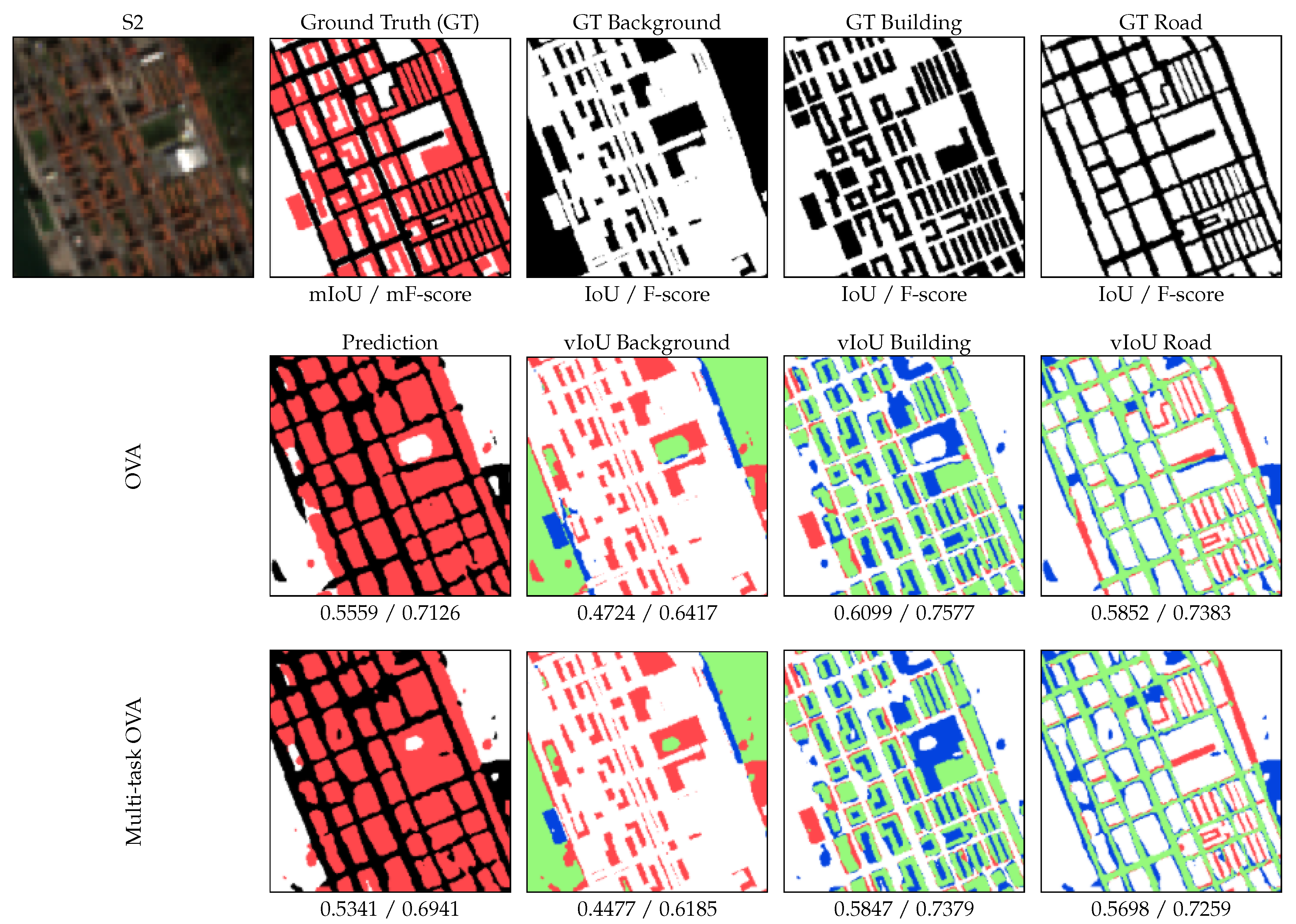
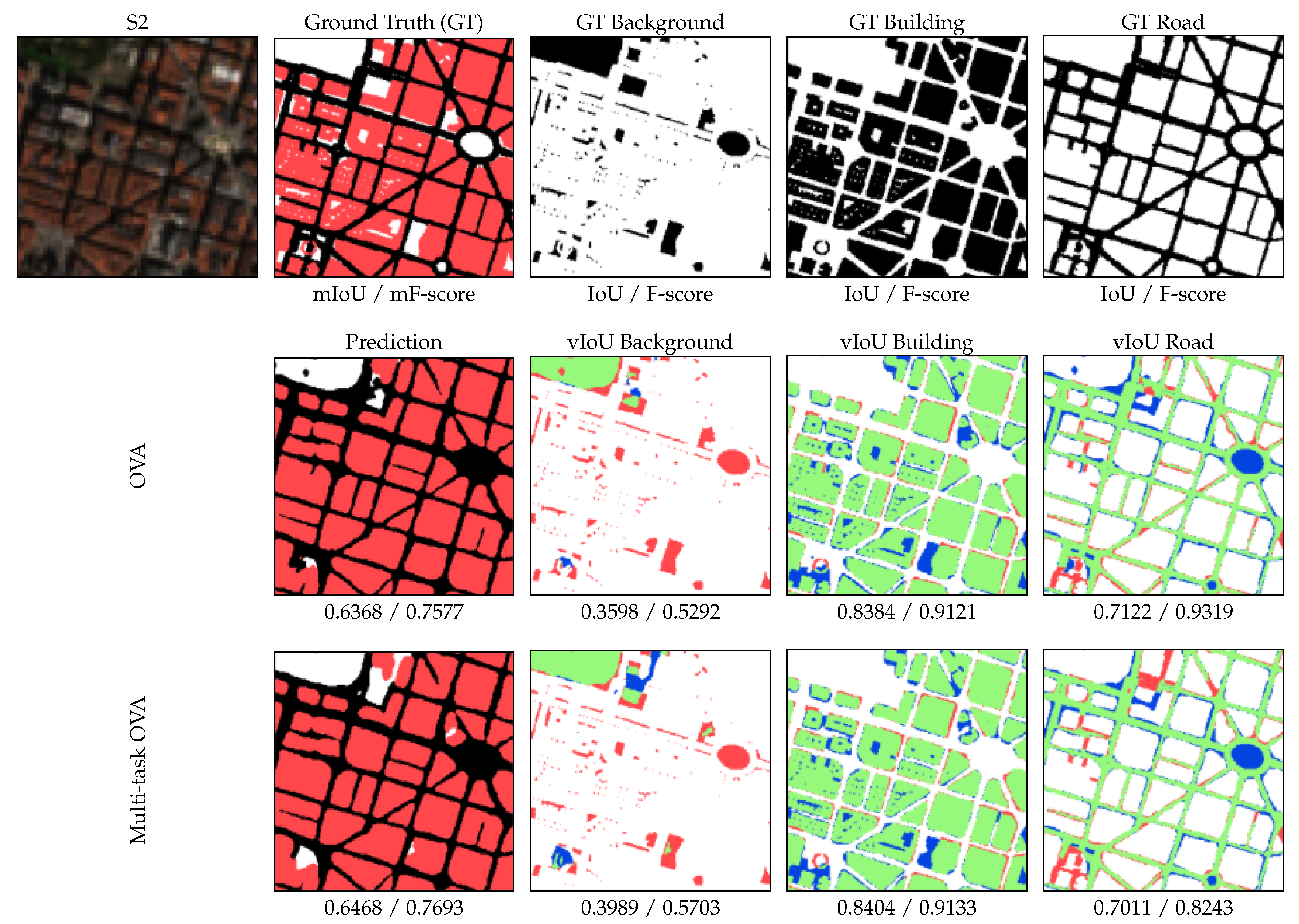
4.2. Experiment 2: Improving the Binary Performance Using a Multi-Task Scheme

The previous experiment has shown the benefits of decomposing a multi-class semantic segmentation problem to reduce its complexity. Moreover, the OVA decomposition strategy has led to better results than its OVO counterpart. In this experiment, we will focus on further improving the results of the OVA model. In this regard, a combination between the OVA model and a multi-task learning scheme will be analyzed. Specifically, it will be studied whether learning not only the main segmentation task, but also a complementary one such as predicting the percentage of annotated pixels can further improve the results. The results obtained in this experiment are presented in Table 3.
Whereas the OVA model performs better in the background and road classes (0.8670 vs. 0.8631, and 0.5828 vs. 0.5698, in terms of averaged IoU, and 0.9287 vs. 0.9264, and 0.7347 vs. 0.7252, in terms of averaged F-score, for both classes, respectively), its combination with a multi-task learning scheme leads to better results in the building class (0.5954 vs. 0.5789, and 0.7450 vs. 0.7325, in terms of averaged IoU and F-score, respectively).
Figure 9 and Figure 10 set out a visual comparison between the OVA binary decomposition strategy and its combination with a multi-task learning scheme.
Closely looking to these figures, one draws the similar conclusions to the ones extracted from the previous table with extra information. Although both approaches perform similarly overall, the multi-task variant reduces the number of false positives in the background and road classes. However, the number of false positives is increased in the building class.

5. Conclusions and Future Work

In this work, an in-depth study is carried out in order to determine how a remote sensing multi-class semantic segmentation problem should be properly tackled. We have focused on high-resolution satellite imagery, since the limited spatial resolution reduces the separability of the classes. In this way, we set a challenging scenario for evaluating the usefulness of the different approaches included in this study.
Specifically, the joint building footprint and road network detection in high-resolution satellite imagery is addressed. For this purpose, a dataset combining S1 and S2 high-resolution satellite imagery with OSM building and road labels is generated. The direct multi-class approach is compared to the OVO and OVA binary decomposition strategies as well as their combination with a multi-task learning hard parameter sharing scheme. Quantitative and qualitative results show that decomposing a multi-class problem into multiple binary ones using an OVA binary decomposition strategy leads to better results than the standard direct multi-class approach. Moreover, despite obtaining similar results overall, multi-task learning seems promising for pushing the performance of binary segmentation models. Therefore, more advanced auxiliary tasks may be taken into consideration for a clear pay-off.
Furthermore, more experimentation is required to properly assess the effect that the number of classes has on the usefulness of the decomposition strategy. Moreover, the dataset could be extended to other cities different from the ones used for training and testing the models. This outlook will not only have a positive effect on the generation capability of the models, but it will also make the evaluation fairer, giving more weight to the conclusions extracted.

Author Contributions

Formal analysis, C.A. (Christian Ayala); Investigation, C.A. (Christian Ayala); Supervision, C.A. (Carlos Aranda) and M.G.; Writing—original draft, C.A. (Christian Ayala); Writing—review & editing, M.G. All authors have read and agreed to the published version of the manuscript.

Funding

This research received no external funding.

Institutional Review Board Statement

Not applicable.

Informed Consent Statement

Not applicable.

Acknowledgments

Christian Ayala was partially supported by the Goverment of Navarra under the industrial PhD program 2020 reference 0011-1408-2020-000008. Mikel Galar was partially supported by Tracasa Instrumental S.L. under projects OTRI 2018-901-073, OTRI 2019-901-091 and OTRI 2020-901-050, and by the Spanish MICIN (PID2019-108392GB-I00/AEI/10.13039/501100011033).

Conflicts of Interest

The authors declare no conflict of interest.

References

  1. Bengio, Y. Deep learning of Representations: Looking Forward. Lecture Notes in Computer Science (Including Subseries Lecture Notes in Artificial Intelligence and Lecture Notes in Bioinformatics). 2013. Available online: https://link.springer.com/chapter/10.1007/978-3-642-39593-2_1 (accessed on 6 September 2021).
  2. Lecun, Y.; Bengio, Y.; Hinton, G. Deep Learning. Nature 2015, 521, 436–444. [Google Scholar] [CrossRef]
  3. Deng, J.; Dong, W.; Socher, R.; Li, L.; Li, K.; Li, F.-F. ImageNet: A large-scale hierarchical image database. In Proceedings of the 2009 IEEE Conference on Computer Vision and Pattern Recognition, Miami, FL, USA, 20–25 June 2009; pp. 248–255. [Google Scholar]
  4. Cordts, M.; Omran, M.; Ramos, S.; Rehfeld, T.; Enzweiler, M.; Benenson, R.; Franke, U.; Roth, S.; Schiele, B. The Cityscapes Dataset for Semantic Urban Scene Understanding. In Proceedings of the IEEE Conference on Computer Vision and Pattern Recognition (CVPR), Las Vegas, NV, USA, 27–30 June 2016. [Google Scholar]
  5. Lin, T.; Maire, M.; Belongie, S.; Bourdev, L.; Girshick, R.; Hays, J.; Perona, P.; Ramanan, D.; Zitnick, C.L.; Dollár, P. Microsoft COCO: Common Objects in Context. arXiv 2014, arXiv:1405.0312. [Google Scholar]
  6. Krizhevsky, A.; Sutskever, I.; Hinton, G.E. ImageNet classification with deep convolutional neural networks. Commun. ACM 2017, 60, 84–90. [Google Scholar] [CrossRef]
  7. Voulodimos, A.; Doulamis, N.; Doulamis, A.; Protopapadakis, E. Deep Learning for Computer Vision: A Brief Review. Comput. Intell. Neurosci. 2018, 2018, 7068349. [Google Scholar] [CrossRef]
  8. Shrestha, A.; Mahmood, A. Review of Deep Learning Algorithms and Architectures. IEEE Access 2019, 7, 53040–53065. [Google Scholar] [CrossRef]
  9. Abadi, M.; Barham, P.; Chen, J.; Chen, Z.; Davis, A.; Dean, J.; Devin, M.; Ghemawat, S.; Irving, G.; Isard, M.; et al. TensorFlow: A system for large-scale machine learning. In Proceedings of the 12th USENIX Symposium on Operating Systems Design and Implementation (OSDI 2016), Savannah, GA, USA, 2–4 November 2016. [Google Scholar]
  10. Team, T.T.D. Theano: A Python framework for fast computation of mathematical expressions. arXiv 2016, arXiv:1605.02688. [Google Scholar]
  11. Paszke, A.; Gross, S.; Massa, F.; Lerer, A.; Bradbury, J.; Chanan, G.; Killeen, T.; Lin, Z.; Gimelshein, N.; Antiga, L.; et al. PyTorch: An Imperative Style, High-Performance Deep Learning Library. In Proceedings of the 33rd Conference on Neural Information Processing Systems (NeurIPS 2019), Vancouver, BC, Canada, 8–14 December 2019; Available online: https://proceedings.neurips.cc/paper/2019/file/bdbca288fee7f92f2bfa9f7012727740-Paper.pdf (accessed on 6 September 2021).
  12. Yang, R.; Yu, Y. Artificial Convolutional Neural Network in Object Detection and Semantic Segmentation for Medical Imaging Analysis. Front. Oncol. 2021, 11, 573. [Google Scholar] [CrossRef]
  13. Grigorescu, S.; Trasnea, B.; Cocias, T.; Macesanu, G. A survey of deep learning techniques for autonomous driving. J. Field Robot. 2020, 37, 362–386. [Google Scholar] [CrossRef]
  14. Zhu, X.X.; Tuia, D.; Mou, L.; Xia, G.; Zhang, L.; Xu, F.; Fraundorfer, F. Deep Learning in Remote Sensing: A Comprehensive Review and List of Resources. IEEE Geosci. Remote Sens. Mag. 2017, 5, 8–36. [Google Scholar] [CrossRef] [Green Version]
  15. Zhang, L.; Zhang, L.; Du, B. Deep Learning for Remote Sensing Data: A Technical Tutorial on the State of the Art. IEEE Geosci. Remote Sens. Mag. 2016, 4, 22–40. [Google Scholar] [CrossRef]
  16. Feng, Y.; Yang, C.; Sester, M. Multi-Scale Building Maps from Aerial Imagery. ISPRS—Int. Arch. Photogramm. Remote Sens. Spat. Inf. Sci. 2020, 43, 41–47. [Google Scholar] [CrossRef]
  17. Corbane, C.; Syrris, V.; Sabo, F.; Politis, P.; Melchiorri, M.; Pesaresi, M.; Soille, P.; Kemper, T. Convolutional neural networks for global human settlements mapping from Sentinel-2 satellite imagery. Neural Comput. Appl. 2021, 33, 6697–6720. [Google Scholar] [CrossRef]
  18. Zhang, Z.; Liu, Q.; Wang, Y. Road Extraction by Deep Residual U-Net. IEEE Geosci. Remote Sens. Lett. 2018, 15, 749–753. [Google Scholar] [CrossRef] [Green Version]
  19. Ayala, C.; Aranda, C.; Galar, M. Towards Fine-Grained Road Maps Extraction Using Sentinel-2 Imagery. ISPRS Ann. Photogramm. Remote Sens. Spat. Inf. Sci. 2021, 2021, 9–14. [Google Scholar] [CrossRef]
  20. European Spatial Agency. Copernicus Programme. Available online: https://www.copernicus.eu (accessed on 6 September 2021).
  21. El Mendili, L.; Puissant, A.; Chougrad, M.; Sebari, I. Towards a Multi-Temporal Deep Learning Approach for Mapping Urban Fabric Using Sentinel 2 Images. Remote Sens. 2020, 12, 423. [Google Scholar] [CrossRef] [Green Version]
  22. Oehmcke, S.; Thrysøe, C.; Borgstad, A.; Salles, M.A.V.; Brandt, M.; Gieseke, F. Detecting Hardly Visible Roads in Low-Resolution Satellite Time Series Data. In Proceedings of the 2019 IEEE International Conference on Big Data (Big Data), Los Angeles, CA, USA, 9–12 December 2019; pp. 2403–2412. [Google Scholar]
  23. Alem, A.; Kumar, S. Deep Learning Methods for Land Cover and Land Use Classification in Remote Sensing: A Review. In Proceedings of the 2020 8th International Conference on Reliability, Infocom Technologies and Optimization (Trends and Future Directions) (ICRITO), Noida, India, 4–5 June 2020; pp. 903–908. [Google Scholar]
  24. Ayala, C.; Sesma, R.; Aranda, C.; Galar, M. A Deep Learning Approach to an Enhanced Building Footprint and Road Detection in High-Resolution Satellite Imagery. Remote Sens. 2021, 13, 3135. [Google Scholar] [CrossRef]
  25. Saito, S.; Yamashita, Y.; Aoki, Y. Multiple Object Extraction from Aerial Imagery with Convolutional Neural Networks. J. Imaging Sci. Technol. 2016, 60, 10402. [Google Scholar] [CrossRef]
  26. Lorena, A.; Carvalho, A.; Gama, J. A review on the combination of binary classifiers in multiclass problems. Artif. Intell. Rev. 2008, 30, 19–37. [Google Scholar] [CrossRef]
  27. Zhou, J.T.; Tsang, I.W.; Ho, S.S.; Müller, K.R. N-ary decomposition for multi-class classification. Mach. Learn. 2019, 108, 809–830. [Google Scholar] [CrossRef] [Green Version]
  28. Fernández, A.; López, V.; Galar, M.; del Jesus, M.J.; Herrera, F. Analysing the classification of imbalanced data-sets with multiple classes: Binarization techniques and ad-hoc approaches. Knowl.-Based Syst. 2013, 42, 97–110. [Google Scholar] [CrossRef]
  29. Galar, M.; Fernández, A.; Barrenechea, E.; Bustince, H.; Herrera, F. An overview of ensemble methods for binary classifiers in multi-class problems: Experimental study on one-vs.-one and one-vs.-all schemes. Pattern Recognit. 2011, 44, 1761–1776. [Google Scholar] [CrossRef]
  30. Knerr, S.; Personnaz, L.; Dreyfus, G. Single-layer learning revisited: A stepwise procedure for building and training a neural network. In Neurocomputing; Springer: Berlin/Heidelberg, Germany, 1990; pp. 41–50. [Google Scholar]
  31. Anand, R.; Mehrotra, K.; Mohan, C.; Ranka, S. Efficient classification for multiclass problems using modular neural networks. IEEE Trans. Neural Netw. 1995, 6, 117–124. [Google Scholar] [CrossRef] [PubMed]
  32. Girshick, R. Fast R-CNN. In Proceedings of the 2015 IEEE International Conference on Computer Vision (ICCV), Santiago, Chile, 7–13 December 2015; pp. 1440–1448. [Google Scholar]
  33. Caruana, R. Multitask Learning. Mach. Learn. 1997, 28, 41–75. [Google Scholar] [CrossRef]
  34. Bischke, B.; Helber, P.; Folz, J.; Borth, D.; Dengel, A. Multi-Task Learning for Segmentation of Building Footprints with Deep Neural Networks. In Proceedings of the 2019 IEEE International Conference on Image Processing (ICIP), Taipei, Taiwan, 22–25 September 2019; pp. 1480–1484. [Google Scholar]
  35. Shao, Z.; Zhou, Z.; Huang, X.; Zhang, Y. MRENet: Simultaneous Extraction of Road Surface and Road Centerline in Complex Urban Scenes from Very High-Resolution Images. Remote Sens. 2021, 13, 239. [Google Scholar] [CrossRef]
  36. Xu, Y.; Goodacre, R. On Splitting Training and Validation Set: A Comparative Study of Cross-Validation, Bootstrap and Systematic Sampling for Estimating the Generalization Performance of Supervised Learning. J. Anal. Test. 2018, 2, 249–262. [Google Scholar] [CrossRef] [PubMed] [Green Version]
  37. Long, J.; Shelhamer, E.; Darrell, T. Fully convolutional networks for semantic segmentation. In Proceedings of the IEEE Computer Society Conference on Computer Vision and Pattern Recognition, Boston, MA, USA, 7–12 June 2015. [Google Scholar]
  38. Badrinarayanan, V.; Kendall, A.; Cipolla, R. SegNet: A Deep Convolutional Encoder-Decoder Architecture for Image Segmentation. IEEE Trans. Pattern Anal. Mach. Intell. 2017, 39, 2481–2495. [Google Scholar] [CrossRef] [PubMed]
  39. Chen, L.C.; Papandreou, G.; Kokkinos, I.; Murphy, K.; Yuille, A.L. DeepLab: Semantic Image Segmentation with Deep Convolutional Nets, Atrous Convolution, and Fully Connected CRFs. IEEE Trans. Pattern Anal. Mach. Intell. 2018, 40, 834–848. [Google Scholar] [CrossRef]
  40. Ronneberger, O.; Fischer, P.; Brox, T. U-net: Convolutional Networks for Biomedical Image Segmentation. Lecture Notes in Computer Science (Including Subseries Lecture Notes in Artificial Intelligence and Lecture Notes in Bioinformatics). 2015. Available online: https://link.springer.com/chapter/10.1007/978-3-319-24574-4_28 (accessed on 6 September 2021).
  41. Hüllermeier, E.; Vanderlooy, S. Combining predictions in pairwise classification: An optimal adaptive voting strategy and its relation to weighted voting. Pattern Recognit. 2010, 43, 128–142. [Google Scholar] [CrossRef] [Green Version]
  42. Friedman, J.H. Another Approach to Polychotomous Classification; Technical Report; Department of Statistics, Stanford University: Stanford, CA, USA, 1996. [Google Scholar]
  43. Caruana, R. Multitask Learning: A Knowledge-Based Source of Inductive Bias. In Proceedings of the Tenth International Conference on Machine Learning, Morgan Kaufmann, Amherst, MA, USA, 27–29 July 1993; pp. 41–48. [Google Scholar]
  44. Duong, L.; Cohn, T.; Bird, S.; Cook, P. Low Resource Dependency Parsing: Cross-lingual Parameter Sharing in a Neural Network Parser. In Proceedings of the 53rd Annual Meeting of the Association for Computational Linguistics and the 7th International Joint Conference on Natural Language Processing (Volume 2: Short Papers); Association for Computational Linguistics: Stroudsburg, PA, USA, 2015; pp. 845–850. [Google Scholar]
  45. Maggiori, E.; Tarabalka, Y.; Charpiat, G.; Alliez, P. Convolutional Neural Networks for Large-Scale Remote-Sensing Image Classification. IEEE Trans. Geosci. Remote Sens. 2017, 55, 645–657. [Google Scholar] [CrossRef] [Green Version]
  46. Mnih, V. Machine Learning for Aerial Image Labeling. Ph.D. Thesis, University of Toronto, Toronto, ON, Canada, 2013. [Google Scholar]
  47. Haklay, M.; Weber, P. OpenStreetMap: User-Generated Street Maps. IEEE Pervasive Comput. 2008, 7, 12–18. [Google Scholar] [CrossRef] [Green Version]
  48. Kaiser, P.; Wegner, J.D.; Lucchi, A.; Jaggi, M.; Hofmann, T.; Schindler, K. Learning Aerial Image Segmentation from Online Maps. IEEE Trans. Geosci. Remote Sens. 2017, 55, 6054–6068. [Google Scholar] [CrossRef]
  49. European Spatial Agency. Copernicus Open Access Hub. Available online: https://scihub.copernicus.eu/ (accessed on 6 September 2021).
  50. Filipponi, F. Sentinel-1 GRD Preprocessing Workflow. Proceedings 2019, 18, 11. [Google Scholar] [CrossRef] [Green Version]
  51. Kingma, D.P.; Ba, J.L. Adam: A method for stochastic optimization. In Proceedings of the 3rd International Conference on Learning Representations, ICLR 2015—Conference Track Proceedings, San Diego, CA, USA, 7–9 May 2015. [Google Scholar]
  52. Taghanaki, S.A.; Zheng, Y.; Zhou, S.K.; Georgescu, B.; Sharma, P.; Xu, D.; Comaniciu, D.; Hamarneh, G. Combo Loss: Handling Input and Output Imbalance in Multi-Organ Segmentation. Comput. Med. Imaging Graph. 2019, 75, 24–33. [Google Scholar] [CrossRef] [PubMed] [Green Version]
  53. Diakogiannis, F.I.; Waldner, F.; Caccetta, P.; Wu, C. ResUNet-a: A deep learning framework for semantic segmentation of remotely sensed data. ISPRS J. Photogramm. Remote Sens. 2020, 162, 94–114. [Google Scholar] [CrossRef] [Green Version]
Figure 1. U-net architecture [40] adapted to a multi-class semantic segmentation problem, including building footprints and road networks. Note that the final 1 × 1 convolutional layer performs a classification into 3 classes since the background is also considered.
Applsci 11 08340 g001
Figure 2. OVO decomposition scheme adapted to a multi-class semantic segmentation problem, including building footprints and road networks.
Applsci 11 08340 g002
Figure 3. OVA decomposition scheme adapted to a multi-class semantic segmentation problem, including building footprints and road networks.
Applsci 11 08340 g003
Figure 4. Multi-task architectures depending on how the parameters of the hidden layers are shared.
Applsci 11 08340 g004
Figure 5. Dataset generation pipeline for a generic area of interest.
Applsci 11 08340 g005
Figure 6. Geographical distribution of the dataset (green training set/red testing set).
Applsci 11 08340 g006
Figure 7. Qualitative results for the benefits of using decomposition strategies. Visual comparison of the results obtained with the direct multi-class approach vs. OVA and OVO binary decomposition strategies for a zone taken from Pamplona city in the test set. TP are presented in green, FP in blue, FN in red and TN in white.
Applsci 11 08340 g007
Figure 8. Qualitative results for the benefits of using decomposition strategies. Visual comparison of the results obtained with the direct multi-class approach vs. OVA and OVO binary decomposition strategies for a zone taken from Barcelona North city in the test set. TP are presented in green, FP in blue, FN in red and TN in white.
Applsci 11 08340 g008
Figure 9. Qualitative results for the benefits of using a multi-task learning scheme. Visual comparison of the results obtained with the OVA binary decomposition strategy and its multi-task variant, for a zone taken from Pamplona city in the test set. TP are presented in green, FP in blue, FN in red and TN in white.
Applsci 11 08340 g009
Figure 10. Qualitative results for the benefits of using a multi-task learning scheme. Visual comparison of the results obtained with the OVA binary decomposition strategy and its multi-task variant, for a zone taken from Barcelona North city in the test set. TP are presented in green, FP in blue, FN in red and TN in white.
Applsci 11 08340 g010
Table 1. Summary of the dataset. Overall, the training set is composed of 18 cities (75%), whereas the testing set consists of 6 cities (25%).
Train
CityDimensions
A coruña704 × 576
Albacete1280 × 1152
Alicante1216 × 1472
Barakaldo1088 × 896
Barcelona N.1152 × 1728
Castellón1024 × 1024
Córdoba1088 × 1792
Logroño768 × 960
Madrid N.1920 × 2688
Pamplona1600 × 1536
Pontevedra384 × 512
Rivas-vacía1088 × 1088
Salamanca832 × 960
Santander1152 × 1216
Sevilla2176 × 2368
Valladolid1408 × 1408
Vitoria576 × 896
Zaragoza2304 × 2752
Test
CityDimensionsValid Extension (km2)
BuildingRoad
Bilbao576 × 83231724956
Granada1664 × 160016,87974,333
León1216 × 768115118,934
Lugo768 × 57680983
Madrid S.1280 × 262484,797246,651
Oviedo960 × 896958817,892
Table 2. Results obtained in terms of averaged IoU and F-score metrics, in the testing set for Experiment 1.
IoU
CityMulti-ClassOVOOVA
BackgroundBuildingRoadBackgroundBuildingRoadBackgroundBuildingRoad
Bilbao0.68350.50800.37280.80470.61080.49760.83810.63670.5118
Granada0.63610.32220.34720.85500.57450.50120.88410.56600.5554
Leon0.60870.25080.32170.84850.69440.53550.87560.70200.5826
Lugo0.61050.13330.34720.78590.54940.46050.85010.59320.4798
Madrid S.0.61750.41890.37730.81950.54920.59700.86760.57050.6392
Oviedo0.65650.45740.32720.82390.51600.47500.86040.54300.4894
Average0.63200.39940.35650.82790.56290.54270.86700.57890.5828
F-Score
CityMulti-ClassOVOOVA
BackgroundBuildingRoadBackgroundBuildingRoadBackgroundBuildingRoad
Bilbao0.81190.67360.54310.89180.75740.66410.91190.77710.6764
Granada0.77750.48740.51540.92180.72970.66770.93850.72280.7141
Leon0.75680.40090.48660.91800.81960.69740.93370.82480.7362
Lugo0.75780.23500.51430.88010.70830.63050.91890.74440.6484
Madrid S.0.76350.59040.54790.90080.70880.74760.92910.72650.7799
Oviedo0.79260.62760.49300.90340.68070.64390.92490.70370.6569
Average0.77420.56660.52520.90570.71930.70210.92870.73250.7347
Table 3. Results obtained in terms of IoU and F-score metrics, in the testing set for Experiment 2.
IoU
CityOVAMulti-Task OVA
BackgroundBuildingRoadBackgroundBuildingRoad
Bilbao0.83810.63670.51180.84650.63190.5290
Granada0.88410.56600.55540.87600.65540.5450
Leon0.87560.70200.58260.88800.70700.5849
Lugo0.85010.59320.47980.84280.62130.4865
Madrid S.0.86760.57050.63920.84520.55480.5989
Oviedo0.86040.54300.48940.87810.57320.5371
Average0.86700.57890.58280.86310.59540.5698
F-Score
CityOVAMulti-Task OVA
BackgroundBuildingRoadBackgroundBuildingRoad
Bilbao0.91190.77710.67640.91690.77360.6917
Granada0.93850.72280.71410.93390.79180.7054
Leon0.93370.82480.73620.94070.82820.7381
Lugo0.91890.74440.64840.91470.76590.6545
Madrid S.0.92910.72650.77990.91610.71360.7488
Oviedo0.92490.70370.65690.93510.72840.6985
Average0.92870.73250.73470.92640.74500.7252
Publisher’s Note: MDPI stays neutral with regard to jurisdictional claims in published maps and institutional affiliations.

