A Study of OWA Operators Learned in Convolutional Neural Networks

Abstract

Ordered Weighted Averaging (OWA) operators have been integrated in Convolutional Neural Networks (CNNs) for image classification through the OWA layer. This layer lets the CNN integrate global information about the image in the early stages, where most CNN architectures only allow for the exploitation of local information. As a side effect of this integration, the OWA layer becomes a practical method for the determination of OWA operator weights, which is usually a difficult task that complicates the integration of these operators in other fields. In this paper, we explore the weights learned for the OWA operators inside the OWA layer, characterizing them through their basic properties of orness and dispersion. We also compare them to some families of OWA operators, namely the Binomial OWA operator, the Stancu OWA operator and the exponential RIM OWA operator, finding examples that are currently impossible to generalize through these parameterizations.

1. Introduction

Information fusion refers to the process of combining different sources of information into a single output, which tries to summarize those inputs into a single element. The necessity of fusing information appears in many applications, including sensor fusion, statistical analysis, machine learning, and computer vision, among others. From a theoretical point of view, aggregation functions are the most used mathematical tool to deal with information fusion, especially averaging functions [1], where the arithmetic mean and the median are prototypical examples.

A very good example of this averaging functions is the Ordered Weighted Averaging operators (OWA) [2,3]. These are a very well-known family of parameterized class of aggregation operators, which have been commonly applied in several fields, such as multi-criteria decision making or fuzzy logic [4,5]. OWA operators can generalize a large array of aggregations, such as the minimum, the maximum, or the median, among others. This ability to represent very different aggregations has one downside, namely the difficulty of determining the specific weights for an OWA operator in a given context, leading to the development of several methods to establish their parameters [6,7,8,9]. Most of these methods [6] are based on translating the opinion of an expert to a specific weighting vector, usually restricting the natural complexity of the operator to a family of OWAs that are easier to parameterize . In other proposals, the weights are obtained from data [8,9], but even in most of these proposals, the OWA operators are still constrained to parameterized variants.

In this work, we focus on the integration of OWA operators in Machine Learning and Deep Learning, two fields that have grown in importance in recent years. Machine Learning is the study of algorithms capable of learning from data [10]. With the increasing number of data available, developing methods capable of extracting knowledge and exploiting that information has become one of the main topics in the field. One of these methods are Neural Networks (NN), and in particular Deep Learning (DL), which comprises the training of large NNs over large sets of unstructured data.

One of the most successful types of NN used in Deep Learning are Convolutional Neural Networks (CNNs) [11,12]. CNNs are Neural Networks designed for the processing of spatial data, such as images, where any piece of the input information is strongly correlated to other nearby pieces, which form the neighborhood. This fact is usually exploited by CNNs by using convolutional operations that impose local connectivity constraints on the network weights. This results in layers of processing that only exploit local information, ignoring the global perspective of the data, which only gets considered in the final layers of the network.

Aiming at integrating OWA operators in CNNs to improve the performance of CNNs in image classification problems, in a previous work [13], we introduced the OWA layer. The OWA layer modifies the usual CNN architecture by using OWA operators capable of aggregating the feature maps of a CNN based on global information (feature map metrics), even when inserted in the early layers of the network. This modification tries to improve the neighborhood analysis performed by the early convolutional layers of the network by leveraging contextual information about the whole image. Furthermore, the specific implementation proposed is designed to only provide new information without replacing the information already present, minimizing the possibility of any negative impact in the network expressivity.

The proposed layer learns its weights at the same time as the rest of the parameters in the CNN, unlike previous proposals of integration of OWA operators into NNs [14,15,16,17,18,19,20], where the OWA operators are considered independently from the network. These previous methods used predetermined weights or independent training methods for the parameters of the NN and the OWA weighting vector [15,16,17,21]. This difference makes the analysis of the learned OWA operators especially interesting and lets us test whether usually employed parameterized families of OWAs are expressive enough, or if directly learning the operator weights results in wider range of OWAs. In particular, we compare the learned operators with three families of OWA operators, the Binomial OWA [8], the Stancu OWA [22], and the exponential RIM OWA [23].

Therefore, in this work, we elaborate on our previous work focusing on the study of the OWA operators learned with the OWA layer and compare their properties to other classical OWA operator families. To perform this analysis, we focus on the orness and dispersion profiles of the learned operators, two measures introduced by Yager [2] that characterize OWA operators in their closeness to the max operator and the concentration of the weights.

In our previous work [13], we already showed how the OWA layer added new knowledge to a mid-size CNN (based on the VGG13 architecture) on a relatively large dataset. In this work, instead, we are interested in the specific operators learned, and we decide to choose a reduced architecture to facilitate the study. In particular, we employ a minimal two-layer CNN and train different configurations on a small image classification dataset, CIFAR100 [24]. This small dataset and the smaller network architecture enables us to do several repetitions of each configuration, letting us aggregate the final weighting matrices for the OWA layer to extract more meaningful conclusions. Although we acknowledge that considering an experimental framework with a single dataset is a limitation of this work, it also enables us to carry out an in-depth study on the characteristics of the OWAs learned, which would not be straightforward considering a variety of scenarios. The findings presented are meant to serve as a foundation for guiding further lines of work, where the OWA layer should be properly analyzed in larger networks and new datasets to corroborate the presented results.

The remainder of this work is as follows. Section 2 introduces some preliminaries on CNNs and OWA operators. In Section 3, we present the literature relevant to our proposal. Section 4 defines our proposed layer architecture and its design. Then, Section 5 presents the experimental implementation that we have chosen and the specific experiments that we use to test the new layer. Section 6 analyzes the results of the experiments, including a detailed analysis of the OWA weighting matrices. Finally, Section 7 summarizes the conclusions of the work and proposes some future research work.

2. Preliminaries

In this Section, we recall several concepts that are the basis for this work. First, we will recall some fundamentals of CNNs in Section 2.1. Next, we will explore the OWA operator and its characteristics in Section 2.2.

2.1. Convolutional Neural Networks

Generally speaking, Neural Networks (NNs) [25] are algorithms developed for pattern recognition. They are built as an aggregation of multiple simpler units, neurons, arranged in a network. These neurons, when properly trained, can specialize in different simple tasks, letting the whole system learn complex behaviors.

One of the key features of these systems is the training algorithm, based in the idea of backpropagation [26]. This algorithm evaluates the network over an input, and then computes the errors between the obtained and expected outputs. These errors are then backpropagated through the network, from output to input, updating all the parameters along the way to increase the system accuracy. This technique enables the training of extremely complex NNs over large datasets.

Different network architectures have been designed for specific purposes. Initially, the Multilayer Perceptron (MLP) [27] was proposed as a multi-purpose neural network. MLPs are dense networks that arrange the neurons in layers, each one fully connected to all the nodes in the next and previous layers. This leads to complex networks with many weights to train. Some architectures try to reduce this complexity according to the constraints of specific problems. Convolutional Neural Networks (CNNs) [11,12] are another well-known variant of NNs where convolutional filters are combined with pooling layers to deal with multidimensional data such as image classification.

There are two main layers that define CNNs, convolutional and pooling layers. Convolutional layers determine the number of convolutions to apply, each one with its independent weights (the convolutional filter). Since each convolution aggregates the input into a single channel image, also known as feature map, the convolutional layer as a whole generates a new image with as many channels as filters are applied in the layer. In these convolutional layers, most of the information is aggregated across channels, while vertically and horizontally the information is aggregated only on the immediate neighborhood of each pixel. This means that the information codified in a single pixel of a feature map comes only from its spatial neighborhood and ignores the rest of the image.

Pooling layers are used to aggregate the information in the spatial dimensions of the image [24]. These layers keep the channels of the image intact and reduce the dimensionality of the image in the vertical and horizontal dimensions. To perform this reduction, blocks of a certain width and height are defined independently for each channel, and the information in those blocks is aggregated to a single element. This aggregation is usually performed using operators such as the maximum or the average, although there has been some work also on the usage of general OWAs [18,19].

In CNNs, by design, the network tends to operate by exploiting local information in the convolutional layers early in the architecture, and aggregating it into global scale information on the later stages of the network, after each application of a pooling layer. The OWA layer studied in this work tries to change this architecture, letting the network learn some global information in the early layers. Examples of this type of architecture specific to the image classification problem are LeNet [28], the VGG family of models [29], ResNet [30], and DenseNet [31], among others.

2.2. Aggregation Functions and OWA Operators

The main mathematical tool to deal with information fusion is the concept of aggregation function.   

Definition 1

(Aggregation function [1,32]). A mapping $f:{[0,1]}^N\to [0,1]$ is called an aggregation function if it satisfies boundary conditions, i.e., $f(0,\dots ,0)=0$ and $f(1,\dots ,1)=1$ , and increasing monotonicity, i.e., if $x_i\le y_i$ for all $i\in \{1,\dots ,N\}$ , then $f(x_1,\dots ,x_N)\le f(y_1,\dots ,y_N)$.

   Aggregation functions encompass many different type of functions, such as t-norms and t-conorms, among others. In this work, however, we focus on a specific type, called averaging functions.   

Definition 2

(Averaging function [33]). An aggregation function $f:{[0,1]}^N\to [0,1]$ is called averaging if $min(x_1,\dots ,x_n)\le f(x_1,\dots ,x_n)\le max(x_1,\dots ,x_n)$ for every $x_1,\dots ,x_n\in {[0,1]}^n$.

Remark 1.

Notice that, although averaging functions are defined on $[0,1]$, their domain can be extended to any subinterval of the real line.

Special cases of averaging functions are the arithmetic mean, the median, the geometric mean, and the OWA operators, which are the basis of this work.

OWA operators were first proposed by Yager [2,3] as a weighted averaging function in which the weights are not associated to a particular input, but to a specific order position based on the input magnitudes. This allows for easy modeling of linguistic terms, especially in the context of linguistic information fusion [4].   

Definition 3

(OWA operator [2,3]). An OWA operator based on the weighting vector $W=[w_1,\dots ,w_n]$ , with the condition $w_i\in [0,1]$ for every $i=1,\dots ,n$ and ${\sum }_{i=1}^n=1$ , is a mapping $F:{\mathcal{R}}^n\to \mathcal{R}$ such that

$$(x_1,\dots ,x_n)=\sum _{i=1}^n{w}_i{x}_{\sigma \left(i\right)},$$

(1)

where $\sigma :\{1,\dots ,n\}\to \{1,\dots ,n\}$ is a permutation such that $x_{\sigma \left(1\right)}\ge \cdots \ge x_{\sigma \left(n\right)}$ .

   Some notable examples of OWA operators are max ($W_{max}=\left[1,0,\dots ,0\right]$), min ($W_{min}=\left[0,\dots ,0,1\right]$), and the arithmetic mean ($W_{avg}=\left[\frac{1}{n},\dots ,\frac{1}{n}\right]$).

In OWA operators, in contrast with the weighted arithmetic mean, the weights are associated with the magnitude of the inputs. However, there are situations in which the weights need to be associated with certain alternative criteria. In order to deal with these situations, an extension of the OWA operator was also introduced, the Induced Ordered Weighted Averaging operators (IOWA) [34]. The IOWA is a general class of OWA operators in which the ordering of the arguments is induced by another variable, called the order-inducing variable. The previous definition of the OWA operator holds, but defining $\sigma :\{1,\dots ,n\}\to \{1,\dots ,n\}$ as a permutation such that $x_{\sigma \left(1\right)}^{\prime }\ge \cdots \ge x_{\sigma \left(n\right)}^{\prime }$, based on a set of induced variables $x_1^{\prime },\dots ,x_n^{\prime }$ that are, in general, different from $x_1,\dots ,x_n$.

In this work, we study the OWA operators inside an OWA layer (presented later in Section 4), where the objective is the aggregation of 2D feature maps, which do not have an inherent linear order structure. This forces us to define several metrics that map the information in a feature map into a single element, which will then induce the order for the OWA operator. Thus, the underlying function for the OWA layer is in fact an IOWA, although we refer to it as OWA for the sake of simplicity.

Observe that the OWA operator allows us to define a wide family of aggregation functions varying from a pure OR operator (maximum) to an AND operator (minimum). In order to characterize the behavior of an OWA operator, Yager introduced two measures  [2], called orness and dispersion.

Orness 

This measure, also called attitudinal character, tells us how close a certain operator is to the max operator, that is, the preference it has for large argument values. It always lies in the range $\left[0,1\right]$. The orness measure of a weighting vector $W\in {[0,1]}^n$ is defined as

$$orness\left(W\right)=\sum _{i=1}^n{w}_i\frac{n-i}{n-1}.$$

(2)

As an example, the orness of the weighting vectors of some classical OWA operators are $orness\left(W_{max}\right)=1$, $orness\left(W_{min}\right)=0$ and $orness\left(W_{avg}\right)=0.5$.

Dispersion 

This measure, explored in depth in [35], gives us an impression of how concentrated the weights of the operator are. For example, the maximum dispersion is obtained with a weighting vector corresponding to the average ($w_i=\frac{1}{n}$ for every $i=1,\dots ,n$), while the minimum is associated with those weighting vectors W where there exists $i\in \{1,\dots ,n\}$ with $w_i=1$ (and $w_j=0$ for every $j\ne i$). In this work, we use the classic dispersion definition

$$dispersion\left(W\right)=-\sum _{i=1}^n{w}_{i}ln\left(w_i\right).$$

(3)

There have been many proposals of OWA operator parameterizations. With these parameterizations, the weight distribution of the operator can be controlled with a few parameters. These methods guarantee that the operator maintains some interesting properties, but at the expense of constraining its expressivity. One of the latest proposals is the Stancu OWA operator [22], which at the same times generalizes an earlier proposal, the Binomial OWA operator [8].

Binomial OWA 

The Binomial OWA operator [8] is based on a binomial distribution, and defined, for every $i=1,\dots ,n$, as

$$w_{i,n}\left(t\right)=\left(\genfrac{}{}{0pt}{}{n-1}{n-i}\right)t^{n-i}{(1-t)}^{i-1}.$$

(4)

Stancu OWA 

The Stancu OWA operator [22] is instead based on Stancu polynomials and defined, for every $i=1,\dots ,n$, as

$$w_{i,n}(t,\alpha )=\frac{\left(\genfrac{}{}{0pt}{}{n-1}{n-i}\right){\prod }_{s=0}^{n-i-1}(t+s\alpha ){\prod }_{s=0}^{i-2}(1-t+s\alpha )}{{\prod }_{s=0}^{n-2}(1+s\alpha )},$$

(5)

where $t\in [0,1]$, $\alpha \ge 0$, and an empty product denotes 1.

Another approach is the definition of weighting vectors guided by fuzzy quantifiers (also known as Regular Increasing Monotone quantifiers or RIM), widely used in the area of multi-criteria decision making [36]. In the literature many families of RIM quantifiers have been proposed [23]. In particular, we focus on exponential RIM quantifiers.

Exponential RIM OWA 

The exponential RIM OWA operator [23] is based on the generating function

$$Q\left(x\right)=\left\{\begin{array}{cc}\frac{a^x-1}{a-1}\hfill & \mathrm{if} a>0 \mathrm{and} a\ne 1,\hfill \\ x\hfill & \mathrm{if} a=1,\hfill \end{array}\right.$$

(6)

with $a=e^{\lambda }$, for a parameter $\lambda \in \mathbb{R}$.

From the generating function $Q\left(x\right)$ of the quantifier, the weights of the associated OWA operator can be obtained as

$$w_i=Q\left(\frac{i}{n}\right)-Q\left(\frac{i-1}{n}\right).$$

(7)

One of the main properties of the RIM quantifiers with exponential generating functions is that they maximize the entropy for a given orness. This property makes them a solution to the MEOWA operator proposed by O’Hagan [37], maybe the most well-known family of OWA operators.

3. Related Work

OWA operators have been widely used since they were first proposed by Yager [2], thanks to their ability to represent and generalize some well-known aggregations and linguistic operators, such as the minimum, the maximum or the median, among others. Many ways of determining their specific weighting vectors have been developed in the literature [6,7,8]. Most of these methods are supervised approaches, focused on translating an expert opinion to a set of weights [6]. These systems for weight determination are often related to specific families of parametric OWAs, where the expressivity of the operator is reduced to adapt to some usual property constraints [7]. Some of these parameterizations [8,22,23] were presented in Section 2.2.

In other problems, where more expressivity is needed, some works have explored ways to determine the weights of the operators from data [9]. In this work, we will focus on this second approach, but integrating the operators in a standard NN backpropagation loop, designed for complex problems with large numbers of data. The combination of OWA operators and NN has also been already explored in the literature [14,15,16,17,18,19,20,21]. Usually, the OWA operator (or other fuzzy measure-based aggregation function) is introduced outside of the classifier [15,16,17,21], for example, to aggregate an ensemble of classifiers, but some other approaches have also been explored [14,18,19,20].

One of the most ambitious proposals of integration methods is the Linear Order Statistic Neuron developed by Veal et al. [14]. In this work, the authors propose an artificial neuron fully based on an OWA operator, modifying the original simple perceptron idea. When assembled into a complete network, these kinds of neurons would probably exhibit very different properties to those of the NNs, although it is a preliminary work.

The most common approach, and arguably the most natural application of OWA operators (and other families of aggregation functions), is the aggregation of the output of multiple classifiers, which can include Neural Networks [15,16,17,21]. In these schemes, each classifier of the ensemble is trained independently from the rest, and the operator is used to aggregate the outputs into a single one, improving the final system accuracy at the expense of increasing the global complexity.

Another approach that has been explored is the integration of a Fuzzy Measure-based operator (of which the OWA operator is a particular case) in the pooling layer of a CNN [18,19]. In this case, the aggregation used to reduce the dimensionality of a feature map in a pooling layer is replaced with other types of aggregations. Specifically, in these works, the authors employed a Choquet-like integral and show an improvement in results compared to the usual mean and max aggregations.

Finally, the main inspiration for this work has been the “Fuzzy Layer” proposed in [20]. In [20], the fuzzy layer is composed of several OWA operators that are applied to the feature maps generated by a convolutional layer, thus generating a set of new fused maps. These feature maps serve as the input to the next layer, completely replacing the original ones. Regarding the selection of the operators, they manually established fixed operators. In contrast, our OWA layer proposal in [13] is also composed of several OWA operators that generate new fused feature maps, but with important differences. With respect to the usage of the new feature maps, in our proposal, the fused feature maps are used to augment the information of the network, preserving the original feature maps. Moreover, we do not fix beforehand the weights of the OWA operators, but instead, we let the network learn them as parameters. This process of automatic weight determination is the focus of this work.

The OWA layer that we explore in this work was previously defined in [13,38], where we presented some preliminary results about the impact of the layer in CNNs. In the previous works, we found an increase in the accuracy of a medium-sized VGG13 network on a large image dataset, but we did not study the learned OWA operators and the way they codify information. In this work, we continue exploring new results, focusing on the analysis of the learned OWA operators. For this analysis, we use a simpler network and the CIFAR100 [24] dataset both to reduce the complexity of the problem and the number of variables involved and to allow for a greater number of repetitions of each experiment.

Additionally, we compare the learned operators of the OWA layer with several theoretical families of OWA operators. In particular, we use the Stancu OWA operator [22], the Binomial OWA operator [8] and the exponential RIM OWA operator [23]. The Stancu OWA operator is based on the Stancu polynomial and is capable of generating infinitely many sets of weights for a specific orness value, defined by a second parameter $\alpha$. At the same time, it also generalizes the Binomial OWA operator [8]. We also compare the learned operators to the exponential RIM OWA operator [23], proposed as a MEOWA [37] operator based on a RIM quantifier.

4. Methods

In this section, we propose our method for developing the OWA layer of a CNN. In Section 4.1, we present the main structure, the OWA Layer that will be integrated into the network. In Section 4.2, we list the different ordering metrics that we can use inside the OWA Layer to sort the feature maps, and Section 4.3 explains the way we perform the aggregation of those feature maps. Finally, Section 4.4 details the initialization of the weight matrix for the OWA operators represented by the layer.

4.1. Layer Structure

We propose the integration of OWA operators in a general CNN via the use of a special OWA layer [13,38]. This layer will be placed inside the convolutional region of the network and will modify the input data, a 3D matrix of activations, by adding newly generated feature maps by means of OWA operators.

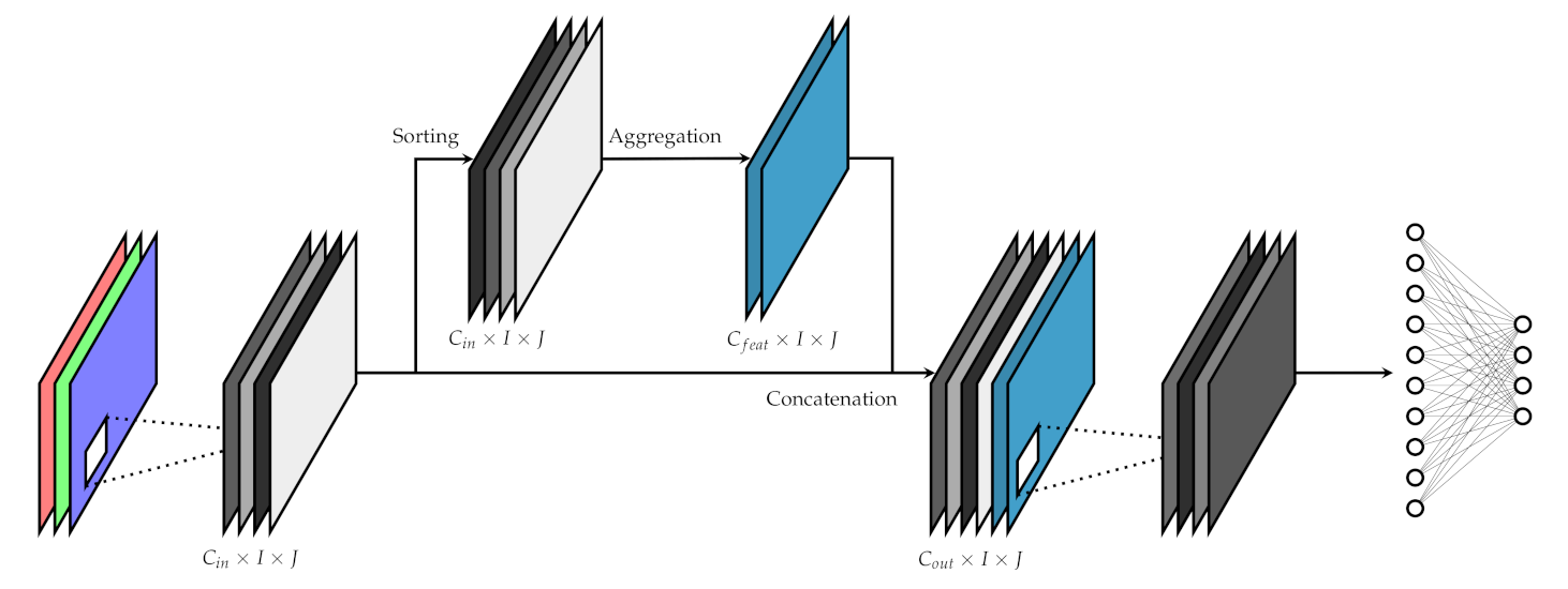
This layer structure responds to our intention of only augmenting the information on the network while using the OWA operators to aggregate the channels based on channel-wise information, usually unavailable to the convolution operation. This way, the layer introduces some of the global scale information codified through channel-wise metrics into the computation of the early layers of the network, which usually exploit only local information. The general structure of the layer is depicted in Figure 1.

This layer takes a 3-dimensional matrix of I rows by J columns by $C_{in}$ channels (feature maps) as input, and appends $C_f$ new channels of the same size to the matrix. Each of the new $C_f$ channels are obtained by aggregating the original $C_{in}$ channels by means of a specific OWA operator. These OWA operators are defined by a weighting matrix of $C_{in}\times C_f$ elements, which are treated as any other parameter in the network and learned through backpropagation.

To apply these OWA operators, two stages are needed. In the first one, we sort the original $C_{in}$ channels is a decreasing order based on a channel-wise metric. Recall that, since we are ordering with respect to a global feature map metric and aggregating channel-wise, we are considering induced OWAs. In the second stage, we perform $C_f$ weighted linear aggregations on the sorted channels. These two steps combined give us $C_f$ independent OWA operators that share the same ordering metric. Finally, these new $C_f$ are concatenated to the original matrix, giving an output with a total of $C_{out}=C_{in}+C_f$ channels.

Note that, in our aggregation proposal, we consider the channel as a whole, rather than aggregating each position $(i,j)$ independently. Thus, we have to carefully define the order metric used for the sorting stage, and the way the aggregation itself is performed, which are not trivial. We elaborate on these issues in the next sections.

4.2. Feature Map Ordering Metrics

As previously explained, our aim is to involve global image information in the feature maps generated in the convolutional part of the CNN. This is done by using OWA operators, whose ordering is given by a channel-wise metric that characterizes the whole channel (feature map). For this, we will use several ordering metrics that assign a real number to each feature map X of dimension $I\times J$. Then, the ordering of the channels is performed by this real number, which represents to some extent the interest in the information stored in the channel. We consider the following metrics:

• Sum, Median and Maximum of channel values. We consider first some of the more classical aggregations. These operators ignore the spatial relationships of the data but still represent the general activation level of the channel.

  $$\mathrm{Sum}\left(X\right)=\sum _{i=1}^I\sum _{j=1}^{J}X(i,j).$$

  (8)

  $$\mathrm{Median}\left(X\right)=median\left(X\right(1,1),\dots ,X(I,J\left)\right).$$

  (9)

  $$\mathrm{Max}\left(X\right)=max\left(X\right(1,1),\dots ,X(I,J\left)\right).$$

  (10)
• Channel entropy. Intuitively, the entropy is a measure of disorder, of the amount of information codified in a channel. A higher value of entropy means more uniformity in the input data, while a smaller entropy value means more contrast and information in that input. For feature maps, we can argue that the entropy of the channel is a good indicator of how interesting the information in the channel is. To compute this metric, we first normalize each element $X(i,j)$ of the channel with the softmax function:

  $$X^{\prime }(i,j)=\mathrm{Softmax}\left(X(i,j)\right)=\frac{e^{X(i,j)}}{{\sum }_{k=1}^I{\sum }_{l=1}^J{e}^{X(k,l)}}.$$

  (11)
  After applying it, we have $X^{\prime }(i,j)\in \left[0,1\right]$ and ${\sum }_{i=1}^I{\sum }_{j=1}^J{X}^{\prime }(i,j)=1$. Then, we can apply the Shannon entropy [39] formula to these values by

  $$H\left(X\right)=-\sum _{i=1}^I\sum _{j=1}^J{X}^{\prime }(i,j)log{X}^{\prime }(i,j).$$

  (12)
• Spatial variation entropy. Generally speaking, the entropy of an information source depends on the codification chosen for it. As the channel values are usually spatially correlated, like an image, we can consider a codification that takes these relationships into account. To obtain the corresponding entropy value, we first compute the horizontal and vertical variations of each position $(i,j)$ of the channel, which are given, respectively, by

  $$V_h\left(X\right)(i,j)=|X(i,j)-X(i-1,j)|\mathrm{for}\mathrm{every}i=2,\dots ,I,j=1,\dots ,J,$$

  (13)

  and

  $$V_v\left(X\right)(i,j)=|X(i,j)-X(i,j-1)|\mathrm{for}\mathrm{every}i=1,\dots ,I,j=2,\dots ,J.$$

  (14)
  We flatten and concatenate all the differences together into a $2IJ-I-J$ length vector V. Then, we proceed normally, applying the softmax function for every j in V:

  $$V^{\prime }\left(j\right)=\mathrm{Softmax}\left(V\left(j\right)\right)=\frac{e^{V\left(j\right)}}{{\sum }_{i=1}^{2IJ-I-J}{e}^{V\left(i\right)}}.$$

  (15)
  Then, we apply the Shannon entropy [39] formula to these normalized variation values by

  $$H_{sv}\left(X\right)=-\sum _{i=1}^{2IJ-I-J}{V}^{\prime }\left(i\right)log{V}^{\prime }\left(i\right).$$

  (16)
• Total variation. The Total variation (TV), as defined in [40], is a metric that conveys similar information to the entropy for spatially constrained data. It tells us how much variance there is between a pixel and its neighbors, being high for images with crisp borders, and low for uniform images. For this metric, we calculate the differences between each pixel and its horizontal and vertical neighbors and aggregate the absolute differences over the image. This is done in the following three steps:

  $${\mathrm{TV}}_v\left(X\right)=\sum _{i=2}^I\sum _{j=1}^J|X(i,j)-X(i-1,j)|,$$

  (17)

  $${\mathrm{TV}}_h\left(X\right)=\sum _{i=1}^I\sum _{j=2}^J|X(i,j)-X(i,j-1)|,$$

  (18)

  $$\mathrm{TV}\left(X\right)=T{V}_v\left(X\right)+T{V}_h\left(X\right).$$

  (19)

4.3. Feature Map Weighted Aggregation

Once the $C_{in}$ input channels have been sorted by one of the measures of Section 4.2, we can proceed to the second critical stage, their weighted aggregation. For this purpose, we define $C_f$ independent OWA operators, each one represented by a weighting vector composed of $C_{in}$ weights.

These weights constitute a raw unconstrained version of the OWA, and we transform them before applying the aggregation to ensure that they correspond to proper weighting vectors. The main reason to work with the weights in their unconstrained form is to easily integrate them into the main backpropagation loop, allowing them to be learned with the rest of the parameters in the network.

To translate the weights into a valid OWA operator, as defined in Section 2.2, we need to ensure that $w_i\in [0,1]$ for every $i=1,\dots ,n$ and that ${\sum }_{i=1}^n=1$. The easiest way to comply with these constraints is to first clip the negative weights to achieve $w_i\in [0,\infty )$ for every $i=1,\dots ,n$, and then normalize to guarantee ${\sum }_{i=1}^n=1$, which implicitly ensures that $w_i\in [0,1]$ for every $i=1,\dots ,n$.

To clip the negative weights, we employ the ReLU function. This is a well-known function that integrates well in the common gradient descent learning algorithm, with a very fast implementation. It is defined as

$$ReLU\left(w_i\right)=max(w_i,0) \mathrm{for} \mathrm{every} i=1,\dots ,C_{in}.$$

(20)

Then, we normalize the weights by dividing each weight by the total sum of the weights, ensuring that the weighting vector adds up to one. The final weights are calculated as

$$w_i^{\prime }=\frac{ReLU\left(w_i\right)}{{\sum }_{j=1}^{C_f}ReLU\left(w_j\right)} \mathrm{for} \mathrm{every} i=1,\dots ,C_{in}.$$

(21)

The resulting weighting vector is a proper OWA weighting vector.

With the final set of $C_f$ weighting vectors calculated, which can be seen as weighting matrix of size $C_f\times C_{in}$, the aggregation itself is straightforward. Each new channel $Y_k$, $k=1,\dots ,C_f$, is given by

$$Y_k(i,j)=\sum _{l=1}^{C_{in}}{w}_l^{\prime }\times X_{\sigma \left(l\right)}(i,j),$$

(22)

for every $i=1,\dots ,I$, $j=1,\dots ,J$. The input feature maps $X_{\sigma \left(l\right)}$ are sorted according to one of the channel metrics presented in Section 4.2, defining a permutation $\sigma \left(l\right)$ such that $\mathrm{Metric}\left(X_{\sigma \left(1\right)}\right)\ge \cdots \ge \mathrm{Metric}\left(X_{\sigma \left(n\right)}\right)$.

4.4. Weight Matrix Initialization

The last key factor in the OWA layer is the initialization of the weighting matrix. The weights, as explained in Section 4.3, are transformed before applying them. This results in an increased operation stack in the backpropagation calculation, meaning that a correct initialization of these weights is vital to allow their convergence to meaningful operators. Most early work in NNs used Gaussian initialization with fixed parameters [24], but recent works have proven the importance of a good initialization [41].

In our case, to approach this problem, we decide to initialize the weights with the absolute value of a Gaussian distribution, keeping the mean at 0 and controlling the standard deviation through a parameter $\alpha$, with $\alpha >0$. This way, we ensure that they are initially positive, and at the same time we can check experimentally for the optimal value of $\alpha$ to guarantee convergence of the weights in the layer. Each weight of the weight matrix is initialized to

$$w_i=∥\mathcal{N}(0,\frac{1}{{\alpha }^2})∥.$$

(23)

5. Experimental Framework

This section describes the experiments that we perform to test the new architecture and the way they are executed. In Section 5.1, we present the image classification problem to be solved and the dataset employed. Section 5.2 proposes a simple CNN capable of solving this problem, and the specific way we can introduce the new OWA Layer to this network. After that, Section 5.3 gives some specific implementation details, and Section 5.4 specifies the evaluation metrics to be used. Finally, Section 5.5 lists the three main experiments that we performed according to the previous specifications.

5.1. Dataset

For testing the architecture, we choose a small and simple image classification dataset, CIFAR100 [24]. It is a well-known dataset, composed of 60,000 color images in a $32\times 32$ pixel resolution. These images are sorted into 100 balanced classes, each split into a train partition of 500 examples and a test partition of 100 examples.

In this work, our main point of interest is the properties of the OWA operators learned inside the OWA layer. Accordingly, we decide to keep the problem definition narrow and work only on this dataset. This choice facilitates the analysis of the results at the cost of keeping them constrained to this experimental framework. In particular, we choose to focus on an image classification problem as it is one of the most common applications for CNNs. The use of this small dataset allows us to run more configurations and repetitions of each configuration, thus giving us more data to aggregate and analyze.

5.2. CNN Architecture

We designed a small CNN with the minimal size to host the new layer, composed of two convolutional blocks, each one composed of a convolutional filter followed by a batch normalization stage and a ReLU activation layer. After the convolutional stage, we used a simple dense layer as the output. The architecture is summarized in

Table 1. Network architecture.

Name	Kernel Size	Stride	Output Size
input_data	-	-	$32\times 32\times 3$
conv1	$3\times 3$	1	$32\times 32\times 64$
${\mathrm{OWA}}_1$	-	-	$32\times 32\times (64+C_f)$ *
conv2	$3\times 3$	1	$32\times 32\times 64$
maxpool	$2\times 2$	2	$16\times 16\times 64$
flatten	-	-	$16,384$
linear	-	-	100

* The OWA layer produces $C_f$ new channels, but as it concatenates those with the original output of the conv1 layer, its final output has $64+C_f$ channels.

. For a review of the usage of the OWA layer on a larger network, refer to [13].

The choice of the base architecture is again motivated to allow for more repetitions of the experiments. In this case, choosing a minimal architecture also reduces the number of variables involved in the configuration of the OWA layer, allowing us to focus better on the analysis of the learned operators.

With this base architecture, we can insert the proposed layer between the two convolutional blocks, using the 64 channels of the first block as input and generating a new representation with an increased number of channels to use as input in the second convolutional block. This insertion point is denoted as ${\mathrm{OWA}}_1$ in Table 1.

5.3. Training Details

For the implementation of the following experiments we used PyTorch [42] 1.4.0 through the Fastai library [43] in its 1.0.60 version.

We focused on the comparison of the reference architecture and the modified one, studying the impact of the new layer. For this reason, we kept the same hyperparameters consistent thorough the experiments. We used a maximum learning rate of $1\times {10}^{-4}$ with a 1cycle policy for hyperparameter management (as described in [44] and implemented in Fastai). We chose this parameter by using the lr_finder tool in Fastai base, adjusting it for the reference configuration. We also used a batch size of 64 across all experiments, the highest we could fit in our GPU. The reference hardware used to run these experiments consisted of a computer equipped with an Intel(R) Core(TM) i5-8500 CPU, 20 GB of general purpose RAM, and a NVIDIA GeForce RTX 2060 Super GPU with 8 GB VRAM.

We used data augmentation, identical in all experiments, based on the setup proposed in [45]. In particular, we used horizontal flipping with a $0.5$ probability and a random padding and crop by four pixels, both keeping the initial image size of $32\times 32$ pixels.

Our code is available for reproduction at https://github.com/irisdominguez/OWA_Layer, last accessed on 4 August 2021.

5.4. Evaluation

For the evaluation of the impact of the new layer, we compare the final test top five accuracy of the trained CNN with and without the new layer inserted. For each version, we repeated the training from scratch 40 times, each one executing 80 epochs, and evaluate the top five test accuracy at the end. Then, we compute the average top five test accuracy of the 40 repetitions as the base result.

To assert the statistical significance of the results, we also use the non-parametric Mann–Whitney U test [46]. For this test, we consider the null hypothesis that the top five accuracy results of both the reference and the modified architecture top five accuracies come from the same random distribution (double sided), and we require a p-value lower than $0.05$ to consider that there is statistical difference when running the modified architecture.

5.5. Experiments

We designed three experiments to understand the kind of OWA operators learned by the network when different configurations are used. We focus on the initialization parameter $\alpha$, the number of learned features $C_f$, and the sorting metric.

• Initialization and convergence. The first experiment was to determine the optimal initialization variance $\alpha$ of the weighing matrix and gave an initial view on the convergence of the parameters. We chose a fixed ordering metric (Total Variation, as described in Section 4.2) and a fixed number of learned OWAs ($C_f=64$, equal to number of input layers) and tested the effect of a range of $\alpha$ on the final learned weights.
  We then plotted different metrics for each OWA weighting vector (namely, orness and dispersion as described in Section 2) to check if the network was learning a variety of operators or if they were limited in their expressivity.
• Number of operators. The second experiment analyzed the impact of the number of learned operators $C_f$. We performed the experiment with a single ordering metric and fixed initialization and varied $C_f$ from 1 to 64 (the number of input channels). We gathered both the top 5 accuracy results for the network and the orness and dispersion profiles of the different configurations.
• Impact of ordering metric. Finally, for the third experiment, we froze all the parameters except for the ordering metrics presented in Section 4.2. This allowed us to observe the behavior of the network with different global information introduced into the OWA layer through these metrics.
  We analyzed both the orness and dispersion profiles of the operators learned for each different metric.

Additionally, we manually selected some of the learned OWA weighting vectors from the third experiment to compare them with the Binomial OWA, Stancu OWA, and exponential RIM OWA operators defined in Section 2.2.

6. Results and Discussion

In this Section we present and analyze the results of the experiments. In Section 6.1, we present the results of the first experiment regarding the initialization of the weights. Next, in Section 6.2, we study the results of the second experiment, exploring the diversity of the learned operators as we modify the number of learned features. In Section 6.3, we study the third experiment, where we focus on the impact of using different ordering metrics. Finally, Section 6.4 analyzes some OWA operator examples learned in the third experiment and compares them to several parametric OWA families.

6.1. Initialization and Convergence

The top 5 accuracy results of this first experiment are shown in

Table 2. Accuracy results for initialization variants.

Init $\mathit{\alpha }$	Top 5 acc.	p-Value
Reference	$52.17\pm 1.5$
1	$54.28\pm 1.4$	<0.001 *
2	$54.47\pm 1.4$	<0.001 *
4	$53.95\pm 1.5$	<0.001 *
8	$54.50\pm 1.6$	<0.001 *
16	$54.38\pm 1.4$	<0.001 *
32	$54.13\pm 1.7$	<0.001 *
64	$54.61\pm 1.4$	<0.001 *
128	$54.26\pm 1.4$	<0.001 *
256	$54.43\pm 1.3$	<0.001 *
512	$54.49\pm 1.3$	<0.001 *
1024	$54.18\pm 1.7$	<0.001 *

* Results marked with * have better top 5 accuracy than the reference with $p-\mathrm{value}<0.05$.

, where we can observe the final top 5 accuracy of the network when we varied the initialization parameter $\alpha$. Although there is a statistically significant improvement in the top 5 accuracy over the reference of about $2\%$, there is little difference between the different initialization parameters accuracy-wise.

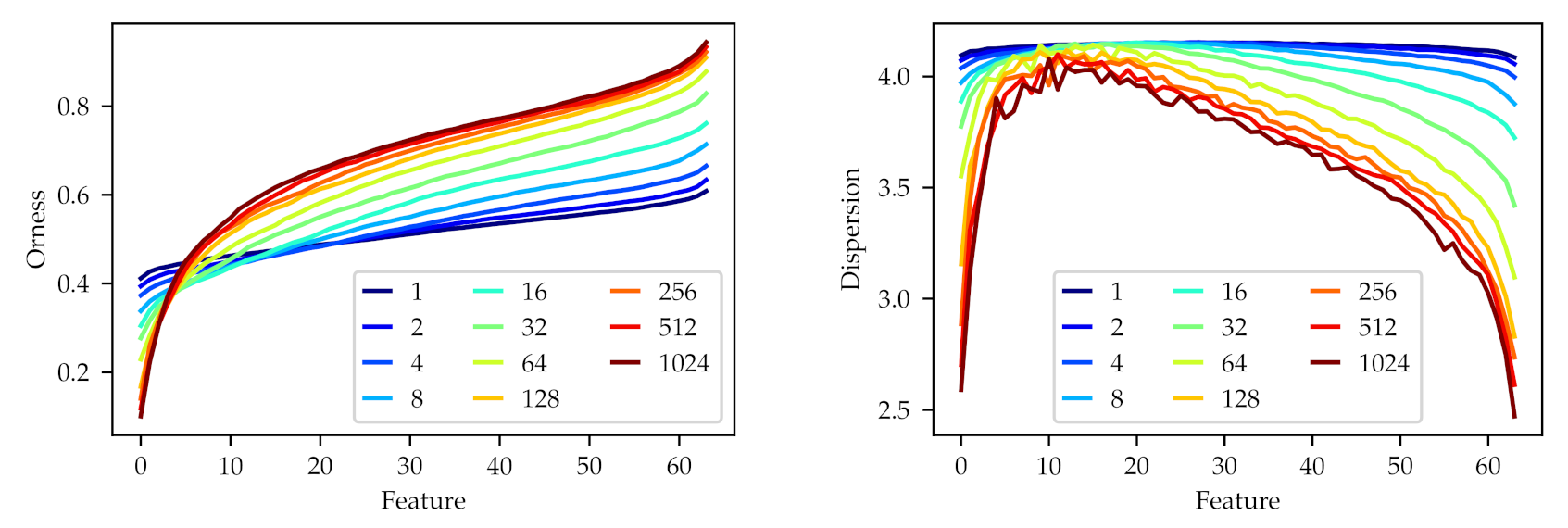
In Figure 2, we focus on the orness and dispersion of the learned features as we vary $\alpha$. To create this figure, we first sorted the operators in each matrix, from lowest to highest orness, and then averaged the 40 weighting matrices of the repetitions of each experiment to denoise them. From this average matrix, we can then computed the orness and dispersion of each operator.

As expected, we can observe how larger values of $\alpha$ (a smaller variance of the initial weights) allows the network to generate a larger diversity of learned features. With an initialization with $\alpha =128$, we already observe an orness range of $0.1$ to $0.9$, covering OWA operators from close to min to close to max. There is a clear tendency to max-like operators, with 54 operators covering the range of ornessess $0.6$ to $0.9$, and only 10 operators in the range $0.1$ to $0.6$ (min-like). We can also observe how lower values of $\alpha$ ($\alpha <128$) have a similar shape in the orness profile, but reduced range, and how higher values ($\alpha >128$) do not increase the range or change the shape of the profile anymore.

About the dispersion, we can observe a maximal value of dispersion (around 4) for the features with an orness close to the average, dropping to lower values of dispersion for the features with minimum and maximum orness. The fact that operators with similar values of orness (operators 10 to 20 on all $\alpha$ configurations show an orness of 0.4 to 0.6) show also a similar value of dispersion suggests a high stability in the shape of the operators across initialization configurations.

Even though these matrices are averaged over the experiments, there is a notable decrease in the stability of the dispersion values for larger values of $\alpha$. This suggests that increasing the value of $\alpha$ not only does not increase the diversity of the operators anymore (as seen on the orness figure) but also leads to noisier and less stable operators.

6.2. Number of Operators

The accuracy results of the second experiment are summarized in

Table 3. Accuracy results by number of learned features.

${\mathit{C}}_{\mathit{f}}$	Top 5 acc.	p-Value
Reference	$52.17\pm 1.5$
1	$52.46\pm 1.4$	$0.331$
2	$52.72\pm 1.7$	$0.176$
4	$53.38\pm 1.3$	<0.001 *
8	$53.18\pm 1.5$	$0.007$ *
16	$53.40\pm 1.2$	<0.001 *
32	$53.74\pm 1.7$	<0.001 *
64	$53.88\pm 1.2$	<0.001 *
128	$55.07\pm 1.4$	<0.001 *
256	$55.03\pm 1.2$	<0.001 *
512	$55.35\pm 1.3$	<0.001 *

* Results marked with * have better top 5 accuracy than the reference with $p-\mathrm{value}<0.05$.

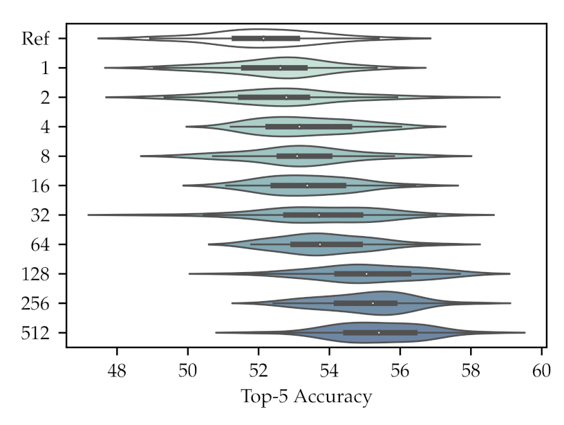
, where the top 5 accuracy of the network, averaged over the 40 repetitions with the same configuration, is shown against the number of learned features $C_f$ introduced in the layer. In this experiment, the sorting metric is the total variation, and $\alpha$ is set to 128. The final top 5 accuracies are also shown as a violin plot in Figure 3, where we can observe a clear correlation between the increase in $C_f$ and the final top 5 accuracy, with all the results with a $C_f>4$ showing a statistically significant result over the reference. The improvement shown reaches $3\%$ over the reference when the highest number of learned features is used. This suggests that adding more operators also increases the knowledge added to the network and proves the diversity of the operators learned in the training.

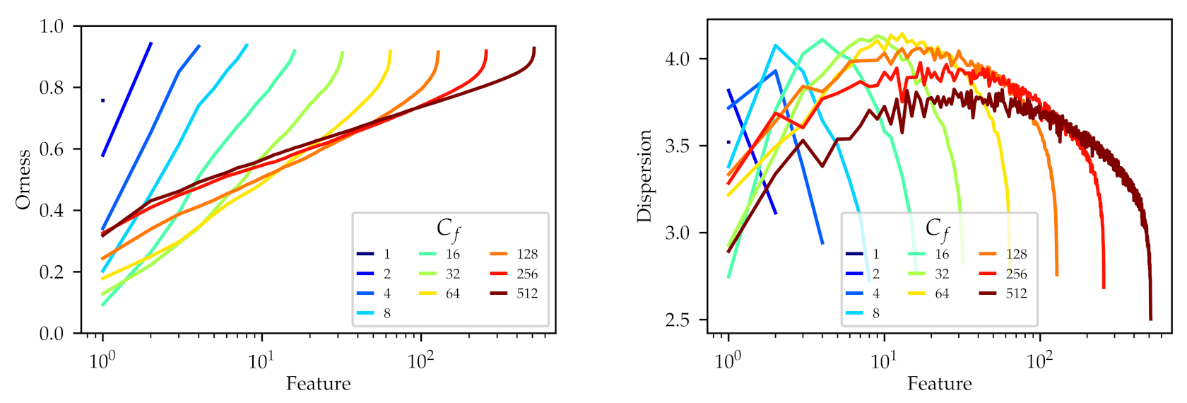
In Figure 4, we show the orness and dispersion profiles of the learned operators, obtained in the same fashion as in Section 6.1. For this figure, considering the variable number of features learned $C_f$, we use a logarithmic horizontal axis to simplify the comparison between different configurations. On the orness profiles, we can observe how, for each number of features $C_f$ from 2 to 16, an increase in the number of features implies an increase in the range of orness. In those cases the upper limit of the profile is close to $1.0$ (max-like), while the lower limit begins at $0.6$ and gets lower with the added features, getting to $0.1$ (min-like) for $C_f=16$. From $C_f=32$ to $C_f=512$, adding new features does not increase the range, and instead reduces it slightly. At $C_f=512$, we can observe that the upper orness limit remains constant, close to $1.0$, but the lower limit has gone back to $0.35$, losing some and-like operators. Recall that in this experiment, the highest $C_f$ were associated with a higher top 5 accuracy.

Reviewing the dispersion profiles in Figure 4, we can observe how, when the orness profile recedes ($C_f=32$ to $C_f=512$), the dispersion of the equivalent operators also decreases. Note how the complete dispersion profile curve becomes lower when $C_f$ becomes higher. This means that the operators learned with higher $C_f$ values are more concentrated, with narrower distributions, even for similar orness values. The learned feature of the highest orness (the last feature of each set) can be noted as an example, sharing a similar orness value for each configuration, but with a decreasing dispersion when the number of features is increased.

These results suggest that learning more OWAs leads the network to explore a certain region of the orness profile meticulously, with many operators that show a low dispersion. In the example configuration, for the total variation metric and $\alpha =128$, this region lies between orness 0.3 and orness 1.0. Recall that this same region was explored by many more operators when we increased the parameter $\alpha$ in the first experiment.

6.3. Impact of Ordering Metric

Finally, the accuracy results of the third experiment are shown in

Table 4. Accuracy results for different metrics.

Metric	Top 5 acc.	p-Value
Reference	$52.17\pm 1.5$
H	$53.78\pm 1.4$	$<0.001$ *
$H_{sv}$	$53.87\pm 1.4$	$<0.001$ *
Sum	$53.93\pm 1.4$	$<0.001$ *
Max	$53.99\pm 1.2$	$<0.001$ *
Median	$54.11\pm 1.1$	$<0.001$ *
TV	$54.27\pm 1.5$	$<0.001$ *

* Results marked with * have better top 5 accuracy than the reference with $p-\mathrm{value}<0.05$.

. Here, we show the average top 5 accuracy of the configuration with the specific ordering metric shown, $\alpha =128$ and $C_f=64$, sorted from lowest to highest accuracy. We can observe statistically significant improvement in all the configurations, but the largest improvements appear with the total variation metric (2% higher than the reference).

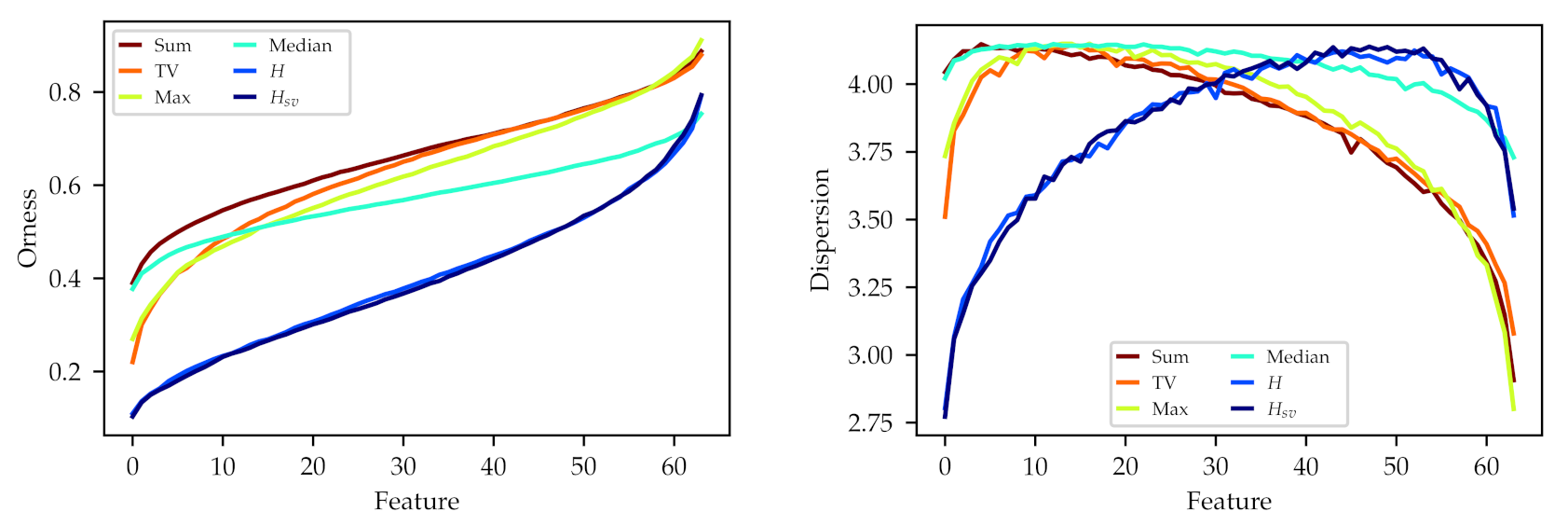
To further explore the differences between the metrics, we show the average orness and dispersion profiles (Figure 5), obtained in the same fashion as in Section 6.1 and Section 6.2. We also show a single example of the resulting weighting matrix of each configuration in Figure 6, each matrix with its features (rows) sorted top to bottom from lowest to highest orness value. These figures show how different ordering metrics tend to converge to different learned features, with different preference for or-like or and-like operators.

We can highlight the two entropy metrics, which both learn a similar distribution of orness slanted to the and-like operators.

A particularly relevant example is the case of the median_activation ordering, which in the matrix shows weight patterns that appear unrelated to the sorting of the layers, and in the orness figure shows the most limited range of all the metrics. This indicates that the median_activation is not adequate to induce the ordering of the channels, making the learned OWAs closer to a regular weighted aggregation. This highlights the importance of the metric selection on the OWA layer to obtain meaningful OWA operators.

6.4. Comparison to Theoretical Families of OWA Operators

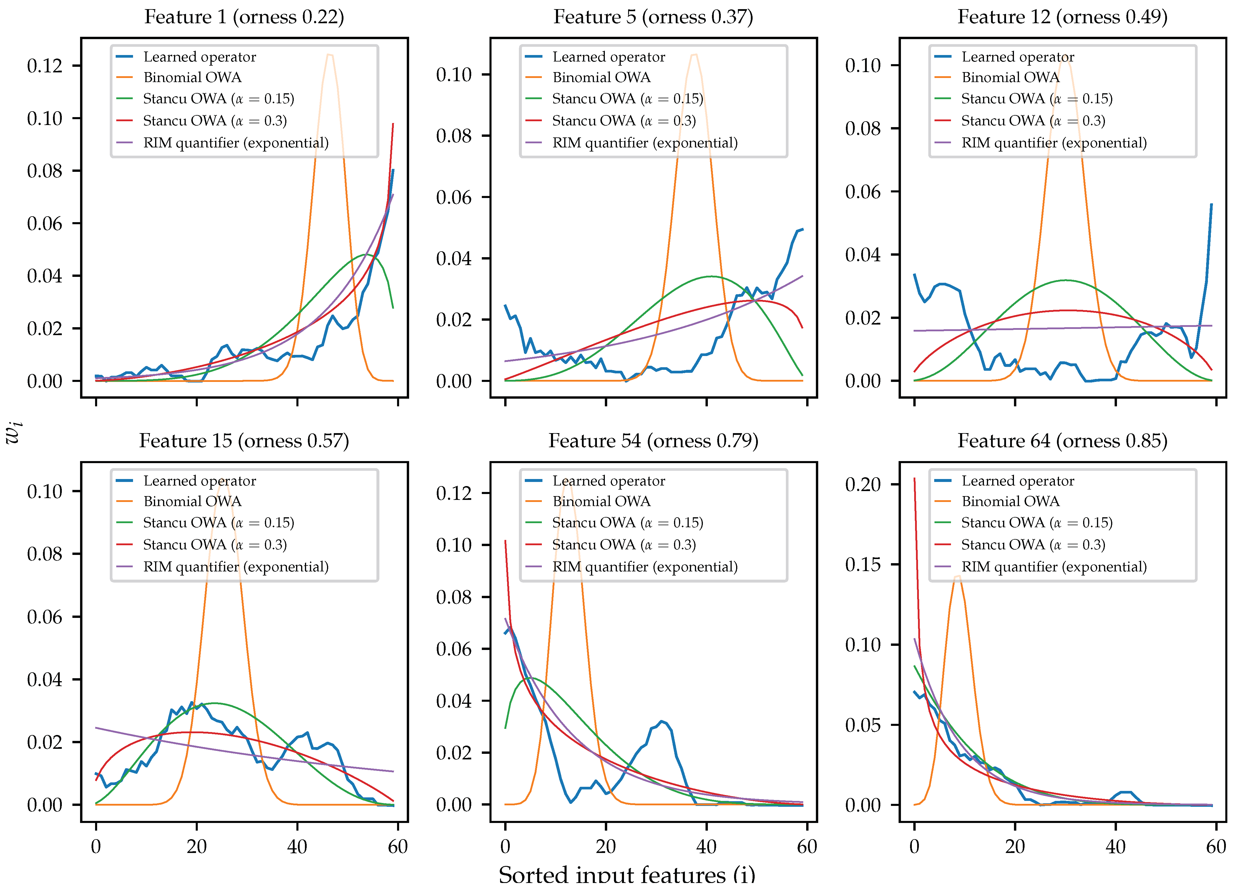
In Figure 7, we show some examples of the operators learned in the third experiment. The raw learned operators are shown filtered to remove noise with a moving average of window size 5. The examples include four examples of parameterized OWA operators of equivalent orness, namely the Binomial OWA, the exponential RIM OWA, and two variants of the Stancu OWA [22] with different $alpha$ values ($\alpha =0.15$ and $\alpha =0.3$).

We can observe how the simpler examples (Features 1 and 64 in the figure) are monotonic and behave very similarly to the Stancu OWA operator and the exponential RIM operator. In the case of Feature 1, with orness $0.22$, the learned operator is best approximated by the Stancu OWA with $\alpha =0.3$, while for the Feature 64, with orness $0.85$, the best approximation would be the Stancu OWA with $\alpha =0.15$. In any case, they can be properly generalized by the Stancu OWA. In both cases, the exponential RIM operator seems to give a very good approximation without the need of any parameter adjustment (it only varies according to orness).

For the other cases, we have chosen a few examples that are harder to generalize. In the case of Features 15 and 54, we can observe how they exhibit a bi-modal weight distribution, a case that cannot be directly modeled with any of the chosen parameterized families of OWA operators. The most extreme examples, Features 5 and 12, show a similar problem, giving most weight to the lowest and highest sorted inputs simultaneously, while giving almost no weight to the intermediate inputs. This is the opposite of a median-like operator, an unusual behavior for the classical OWA operators. We can observe how none of the families can approximate these distributions, especially in the case of the Feature 12, where the best approach is the simple mean represented by the RIM operator.

From these results, we can conclude that the theoretical families of OWA operators currently studied are coherent with many of the data-driven OWA operators learned with OWA layers, but not with all of them. Some of the behaviors shown are currently hard or impossible to model and parameterize with these families, showing room for improvement in terms of expressivity in parameterized OWA families.

7. Conclusions and Future Work

The OWA layer [13] is a CNN layer capable of augmenting the feature maps in a CNN by aggregating them with OWA operators. This leads to an increase in accuracy for CNNs in image classification problems. In this work, we have explored the OWA layer as a way of combining OWA operators with CNNs, with the objective of studying new ways of learning the weights of OWA operators.

First we have confirmed the preliminary results reported in [13,38], observing an improvement in the accuracy of our test network in this specific experimental framework. With respect to our main objective, we have been able to observe how the network generates clean and diverse operators, with orness ranges covering the full spectrum of possibilities. We have also assessed the need for a proper initialization, showing in the first experiment how it can impair the ability of the network to learn diverse operators. The second experiment performed shows how the number of operators learned influences the explored range of possibilities and how the network can extract knowledge even from a small number of operators. Finally, the third experiment has shown how different sorting metrics lead the OWA layer to learn different OWA operators, allowing us to observe how the sorting metric changes the knowledge contributed by the layer.

The most important results, arguably, come from the final comparison between the learned operators and some theoretical families, namely the Binomial OWA [8], the Stancu OWA [22], and the exponential RIM OWA [23]. Our learned operators are empirically consistent with these parameterizations in most cases, but we have also found several examples of operators that are currently impossible to approximate by these families. Considering the nature of the operators learned by the OWA layer, built from scratch and only driven by the data, we believe that this proves a deficiency in the current models. We hope that these results will aid in the design of new models of OWA operators, less constrained and capable of expressing more complex relationships between the input data.

Regarding the OWA layer, we hope that future work will unveil new applications where there is a higher margin of improvement, paving the way to new interactions of OWA operators with other AI tools. The results achieved in this work are still constrained to a narrow experimental framework, and should be extended in future works to new datasets and problems to study the differences in the OWAs learned in different applications as well as the usefulness of the OWA layer. In particular, it would be interesting to study the behavior of the modified CNN when applied to larger datasets, such as ImageNet [47] and its version with reduced image resolution, Tiny ImageNet [48].