Urban Overheating Impact: A Case Study on Building Energy Performance

Abstract

It is well known that the construction sector is one of the main sectors responsible for energy consumption in the current global energy scenario. Thus, buildings’ energy software become essential tools for achieving energy savings. Climate and its implications for building energy performance are a critical threat. Hence, the aim of this study is to evaluate the climatic conditions in urban and suburban areas of Rome, estimating the incidence of the Urban Heat Island (UHI) phenomenon. To this end, meteorological data obtained from three different areas (two airports and one inside the city) were examined and compared. Then, TRNSYS software was used to create a simple building, in order to assess the impacts of various climatic situations on building energy performance. The study revealed significant percentage differences both in terms of energy needs for heating, from −20.1% to −24.9% when the reference stations are, respectively, Fiumicino and Ciampino, and for cooling, with a wider range, from +48.7% to +87.5% when the reference stations are Ciampino and Fiumicino. Therefore, the study showed the importance of more accurately selecting sets of climate values to be included in energy simulations.

1. Introduction

Buildings are the main sector responsible for energy consumption in the current world energy scenario [1]. In this context, energy retrofit interventions and the design of new, efficient buildings prove to be winning strategies.

In particular, building energy simulation software become essential tools for quantifying the energy consumption of green buildings, i.e., of that type of building designed, built and managed in a sustainable and efficient manner, and for assessing the energy savings of existing buildings during the energy requalification phase.

The energy performance of buildings can be assessed using stationary and dynamic simulation codes. These software require specific meteorological data to take into consideration the local environmental climatic conditions, returning the energy demands of the building.

Climate data sets are known as the Typical Meteorological Year (TMY), which is a set of meteorological data characterized by values for each hour in a year, for a given geographic site. The hourly data are chosen over a longer period of time, usually 10 years or more [2]. For each month of the year, data are selected from the year that can be considered most representative for that month. Since 1994, in Italy, buildings have been designed applying the UNI 10349 standard [3]. This is a national standard that suggests monthly average values for climate data for specific sites. Its first version used data from the period 1951–1970. The Standard was updated in 2016 on the basis of the monthly average data calculated from the reference years of the tests developed by CTI [4] for various different Italian cities. Starting from this, it should be noted that nowadays, climate change, and the consequent impact on buildings’ energy performance, represents a critical issue. In fact, urban growth has led to an increase in the air temperature in cities compared to rural areas and to an expansion of the Urban Heat Island (UHI) phenomenon [5,6]. This is caused by the increase in solar radiation absorbed by the building materials [7,8]. The UHI phenomenon increases the cooling in urban areas [9,10], which implies higher energy consumption that leads to an increase in pollutant levels in the urban context [11,12]. Xie et al. [13] studied the correlation between the UHI and the land use/land cover ratio from 1987 to 2016 in Wuhan, China, finding that high temperatures were concentrated in construction land.

The overheating involved in the UHI phenomenon is directly related to human health. As a matter of fact, the increase in air temperature affects the outdoor thermal comfort of inhabitants [14]. This effect is more relevant in summer and, for this reason, making cities cooler plays a crucial role [15].

Therefore, in recent years there has been a significant increase in building retrofit interventions in densely built cities. In fact, in addition to the increasingly widespread use, especially in green buildings, of small renewable generators capable of reducing energy consumption [16] and the attention paid to optimizing the energy tariffs of smart buildings [17], in recent years there have been numerous interventions aimed at reducing energy consumption for cooling and improving the thermal inertia of the building, and studies on the implication of thermostatic appliances (such as air conditioners, water heaters and freezers) on saving electricity in homes, and on safeguarding the internal comfort of the occupants and the internal comfort of the occupants, have intensified [18,19].

Recently, many studies have been focused on mitigation techniques of the UHI, such as green roofs [20,21], cool materials [22,23], vegetation [24,25] and water sources [26,27]. The adoption of mitigation strategies has an important role both for the whole cities and for localized urban areas such as urban canyons [28]. Matias and Lopes [29] studied how the radiation balance of urban materials influences air temperature in an urban canyon.

Consequently, accurate energy modeling becomes essential both for the design of new buildings and for the identification of optimal retrofit interventions.

The presence of a dense and homogeneous distribution of meteorological and climatic stations on the territory, and therefore the availability of numerous climate files, would allow us to conduct more reliable energy simulations in the different study areas and to evaluate in a more realistic way the net transfers of radiative heat between surfaces and the sky vault. In fact, the evaluation of the sky temperature is fundamental too, and must be adequately considered [30].

In addition to quantifying the UHI phenomenon in a typical district of the city of Rome compared to the rural airport areas of Fiumicino and Ciampino, the important novelties of this work consist of underlining the importance of using reliable climate files in building energy simulation software, analyzing the energy needs for heating and cooling and the differences found using different climatic data.

Therefore, the purpose of this study is to evaluate the thermal conditions in urban and suburban areas of Rome, estimating the UHI phenomenon impact. The meteorological data obtained from three different areas of airport and densely built districts of Rome were examined and compared. The differences between the meteorological data were highlighted, also taking into consideration the UNI 10349. Furthermore, the dynamic software TRNSYS [31,32] was used to create a simple building, in order to assess the impact of different climatic situations on the heating and cooling of a reference building.

The paper is structured as follows: Section 2 illustrates the stations from which the climatic data were obtained, the methodology used and the model of the typical building for which the energy needs for cooling and heating were calculated, with the set of climatic data provided as input; Section 3 shows and discusses the results obtained from the study; and finally, Section 4 draws the conclusions.

2. Materials and Methods

Rome is a densely built Italian city of about 4 million inhabitants as a result of a constant urban expansion over time. The city is located 24 km from the Tyrrhenian coast and it is characterized by temperate climatic conditions and hot summer seasons, with maximum average temperatures higher than 30 °C.

To assess the aim of this study, data from different meteorological stations were used: two airport meteorological stations and one urban station (Figure 1).

Specifically, Fiumicino and Ciampino airport stations were selected as they are two rural areas typically also present in the climate data sheets of the dynamic energy modeling software, while the area of the Rome station was selected as it represented a typical neighborhood of the city, densely built and with high population density. This selection made the quantification of the UHI phenomenon realistic and reliable. The airport stations are reference weather stations for the Meteorological Service of the Military Air Force and for the World Meteorological Organization (WMO, Geneva, Switzerland) [33].

The methodological approach of this research can be divided into two main parts:

1. Acquisition and processing of climatic data of the stations selected for the evaluation of the impact of the UHI in Rome;

2. Different climatic conditions’ effects on building energy performance.

Starting from this, the first part of the research is characterized by the following steps:

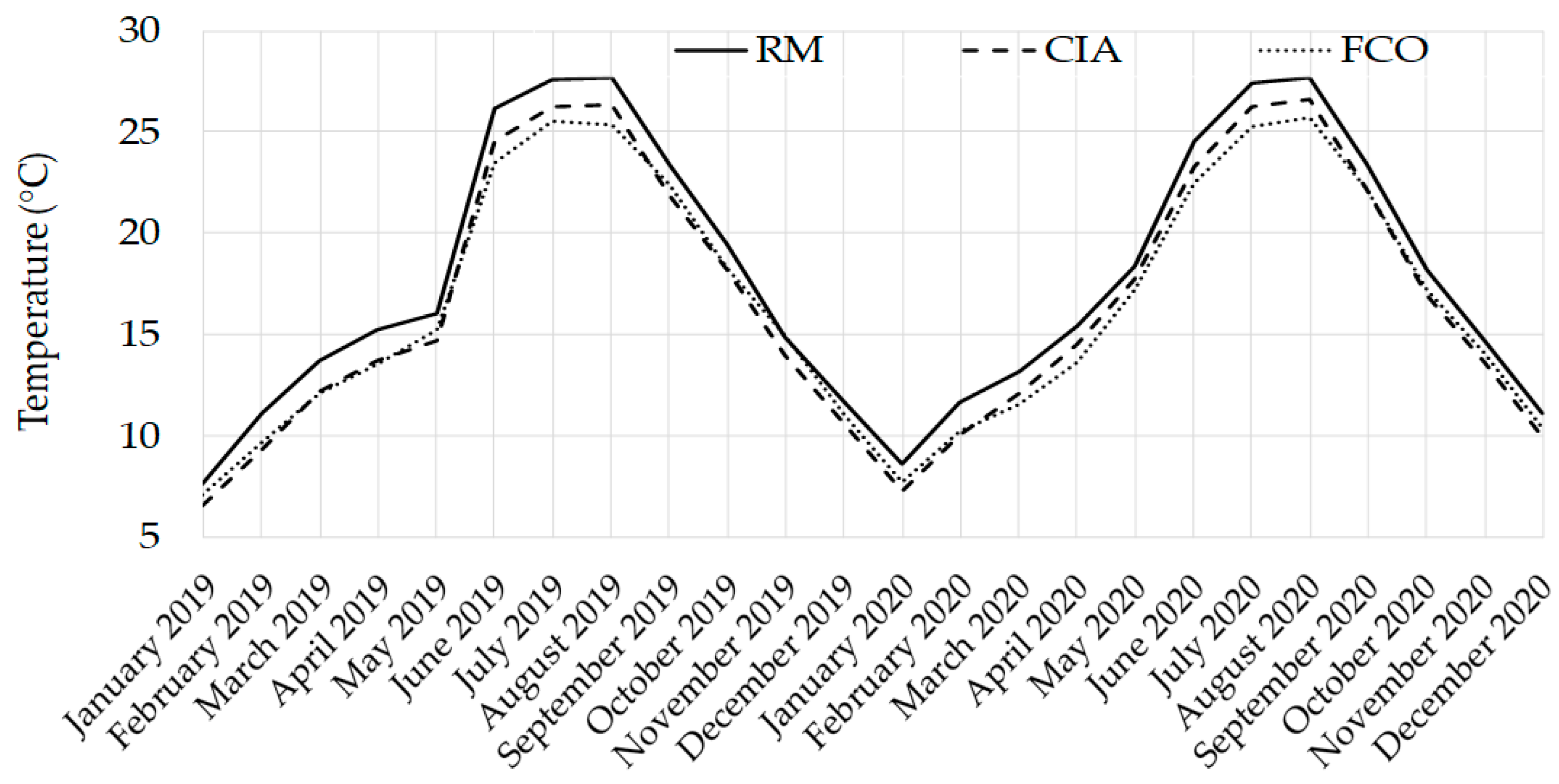
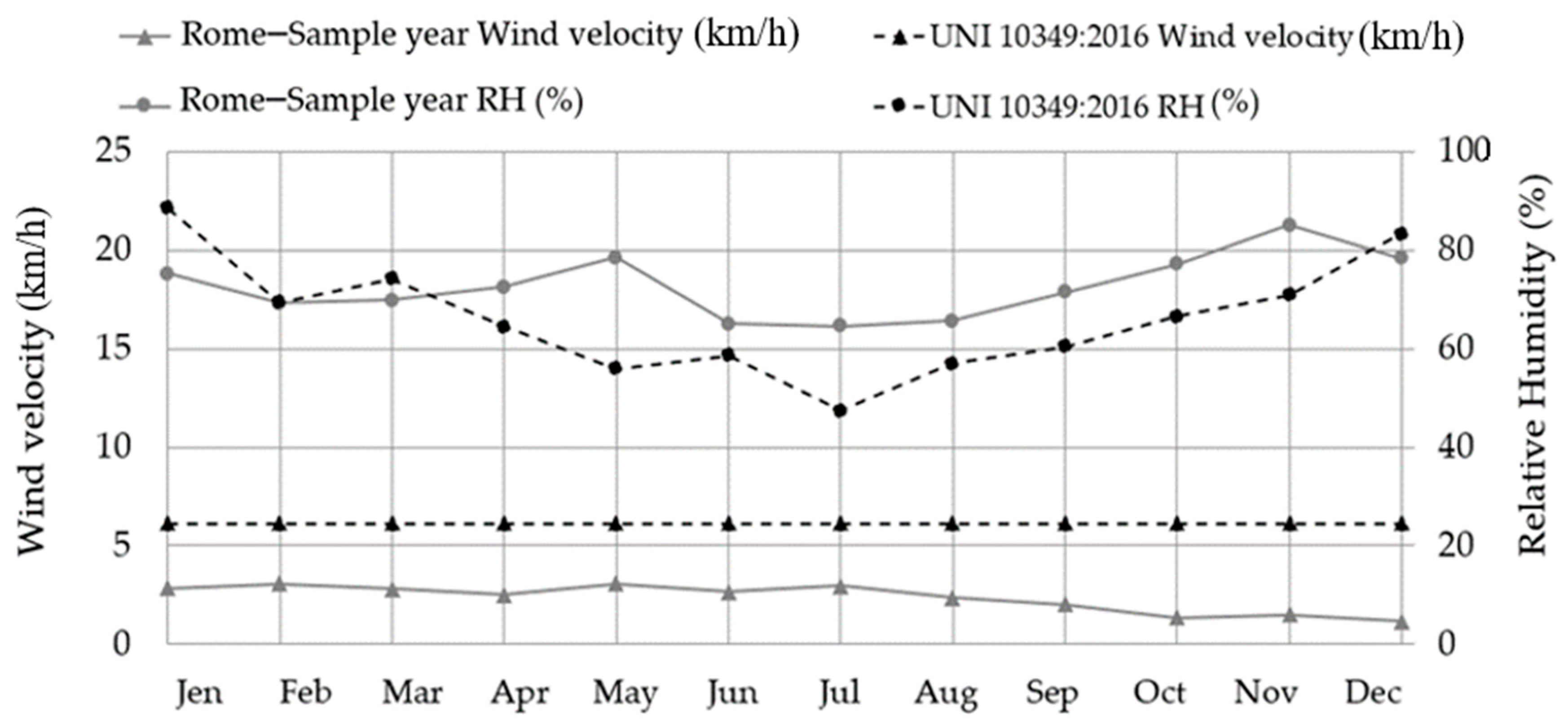
• The biennial meteorological data obtained from two airports near the city (Fiumicino and Ciampino airports) and in a densely built Rome neighborhood were examined and compared considering the same time interval (from January 2019 to December 2020), evaluating the differences in terms of temperature, wind velocity and relative humidity of the three different areas;
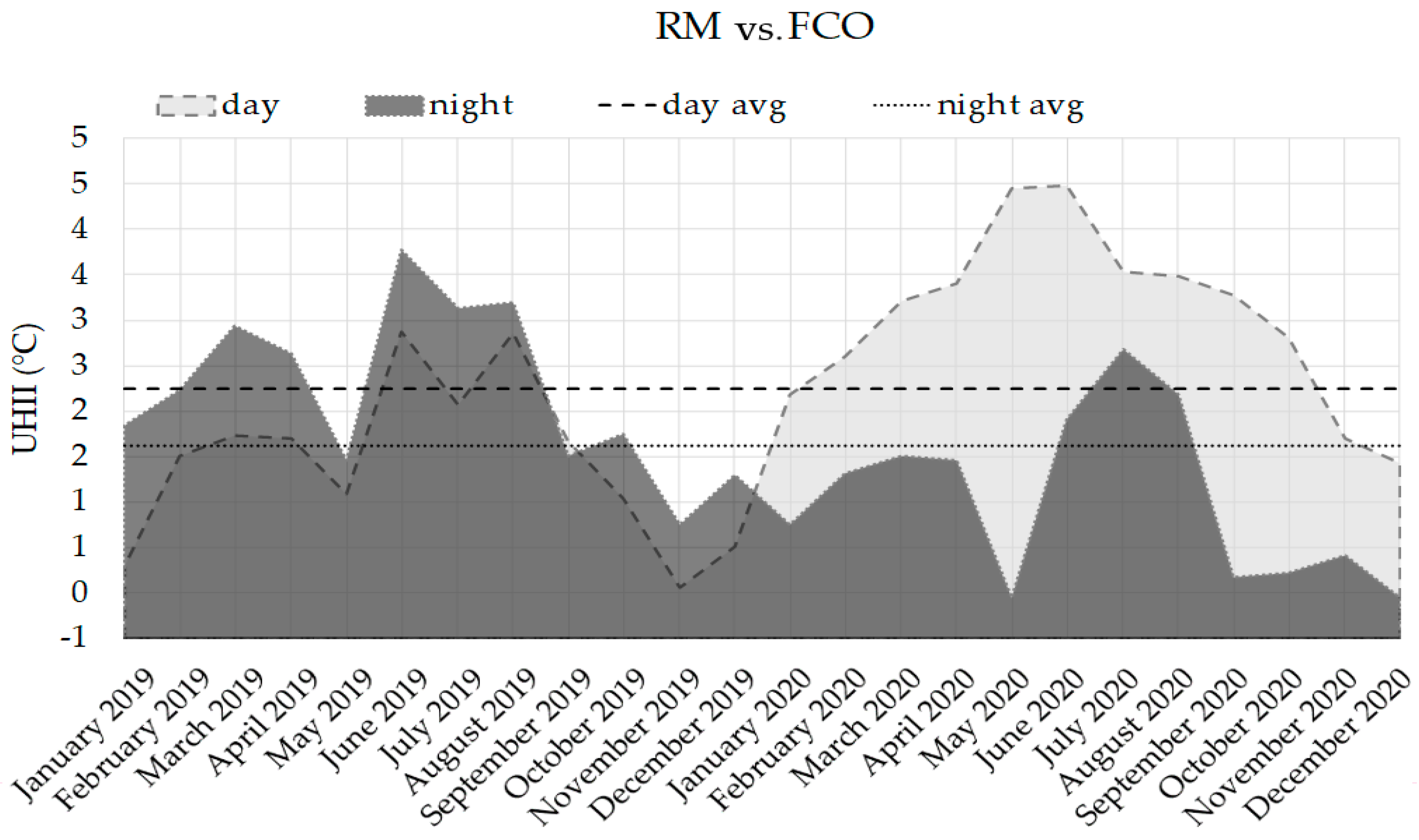
• Monthly average maximum and minimum temperatures were processed and used for evaluating the Urban Heat Island Intensity (UHII) in Rome. In order to quantify the UHI phenomenon, the day and night UHI intensity was used, calculated according to the following expressions:

$$UHI{I}_{day}=Tma{x}_{urban area}-Tma{x}_{rural area}$$

(1)

$$UHI{I}_{night}=Tmi{n}_{urban area}-Tmi{n}_{rural area}$$

(2)

where $UHI{I}_{day} \mathrm{and}$ $UHI{I}_{night}$ are the intensity indices of the UHI phenomenon, diurnal and nocturnal, respectively, $Tma{x}_{urban area} \mathrm{and} Tmi{n}_{urban area}$ are the maximum monthly temperatures recorded during the day and the minimum monthly temperatures recorded at night by the selected Rome station and $Tma{x}_{rural area} \mathrm{and} Tmi{n}_{rural area}$ are the maximum monthly temperatures recorded during the day and the minimum monthly temperatures recorded at night by the rural stations (in this case, one Fiumicino and one Ciampino).

On the other hand, the second part of the research is characterized by the following steps:

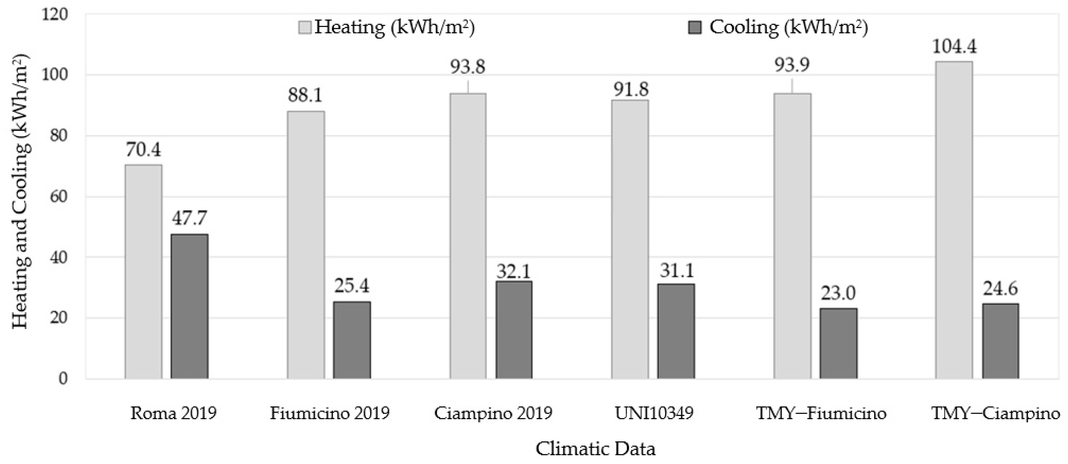
• Analysis of the influence of the different actual weather data recorded in 2019 by the selected stations of Rome, Fiumicino and Ciampino on the annual heating and cooling energy needs of a detached building, through the dynamic software TRNSYS;
• Comparison between the annual heating and cooling energy needs obtained using the TMY available for building energy simulations in Rome, UNI 10349:2016 and actual climatic data in 2019 in order to quantify the differences due to the use of unrealistic climate files.

The stations selected in this study belong to the Davis Vantage Vue model. In particular, the accuracies of the sensors for measuring wind speed and direction, external temperatures and humidity are, respectively, 3 km/h or 5%, 3°, 0.5 °C and 3%. In terms of resolution, the control unit is characterized by values equal to 1 km/h for wind speed, 1° for wind direction, 0.1 °C for external temperature and 1% for relative humidity. Furthermore,

Table 1. Description of the stations used.

Stations	Acronym	m.a.s.l.	Coordinates
Fiumicino	FCO	3 m	41°47′53.66″ N, 12°14′22.36″ E
Ciampino	CIA	129 m	41°48′29.49″ N, 12°35′5.82″ E
Rome	RM	51 m	42°20′22.402″ N, 12°24′35.438″ E

provides information on their positioning.

Energy simulations were performed for a simple, regularly shaped building, characterized by a square plan, with walls with a surface area of 36 m² (see Figure 2). A common wall stratigraphy for the years 1900–1950 was simulated. It is characterized by solid bricks plastered on both sides, with a U-value equal to 1.020 W/m²K. Detailed information about the thicknesses of the layers and the materials’ thermal properties is listed in

Table 2. Wall stratigraphy used in simulations.

Layer	Thickness (m)	Thermal Conductivity (W/mK)	Specific Heat Capacity (J/kgK)	Mass Density (kg/m3)
Plaster	0.02	0.700	1000	1400
Solid bricks	0.58	0.770	840	1600
Plaster	0.02	0.700	1000	1400

.

The whole building envelope had a solar absorptance coefficient equal to 0.6. Windows had an area of 18 m² and a U-value of 5.61 W/m²K. The infiltration rate was equal to 0.5 1/h. Sensible heat equal to 65 W and latent heat equal to 55 W were set for taking into account the occupancy, and thermal power equal to 140 W was set for appliances. The indoor set-point temperatures were 20 °C and 26 °C for heating and cooling, respectively.

3. Results and Discussion

3.1. UHI in Rome: Climatic Data Comparison

The first step of this study focused on the analysis of temperatures, relative humidity and wind speed values registered by the meteorological stations of Rome, Ciampino and Fiumicino during the years 2019 and 2020 (Figure 3, Figure 4 and Figure 5) in order to assess the different climatic scenarios.

Comparing the average monthly air temperatures, the same trend can be observed from Figure 3 for all three selected stations.

In particular, the values obtained from Fiumicino and Ciampino airport stations (renamed in the following figures as “FCO” and “CIA”) are characterized by very similar values during the two years.

On the contrary, air temperatures in Rome are always characterized by higher values, confirming the UHI impact within the city.

The Rome meteorological station was appropriately selected not only for the completeness of the data collected, but also for its central position, in a densely built neighborhood of the city center.

Fiumicino and Ciampino recorded maximum percentage differences in terms of average monthly temperatures equal to 7% in 2019 and 6% in 2020. Fiumicino was characterized by lower temperatures than Ciampino, especially in the summer months of June, July and August, with temperature differences, respectively, equal to 1.07, 0.74 and 1 °C in 2019, and equal to 0.77, 0.94 and 0.92 °C in 2020. In June, July and August, the greatest differences in monthly average temperatures can be noticed when analyzing data related to Rome and Fiumicino. Indeed, for these summer months, the monthly differences are, respectively, equal to 2.68, 2 and 2.29 °C in 2019, and 2.05, 2.14 and 1.97 °C in 2020. By comparing Rome and Ciampino weather data, the greatest temperature differences can be observed during February 2019 (1.81 °C) and February 2020 (1.63 °C).

Furthermore, comparing the average values of the monthly temperatures recorded during 2019 and 2020 by all stations, very low percentage differences can be observed. In particular, they are equal to 0.1% for the Rome station, 1.1% for the Ciampino station and 0.5% for Fiumicino. This was also confirmed by the analysis of the monthly average temperature differences recorded over the two years for each meteorological station. Therefore, the observed temperature trends highlighted the existence of the UHI in Rome. This is also indicated by the wind speed analysis (Figure 4). Significant differences occur due to the different positions of the data acquisition points.

Fiumicino has the highest average wind speed values. During 2019, wind speed values between 10.71 and 16.37 km/h were observed, with an annual mean value of 12.8 km/h. In 2020, values between 11.22 and 14.06 km/h were acquired, with an average wind speed equal to 12.36 km/h. Analyzing Figure 4, wind speeds recorded in Ciampino are higher than those logged in Rome, with an average annual value equal to 10.51 km/h during 2019, and 10.46 km/h during 2020. Rome is characterized by the lowest wind speed values, with annual averages equal to 2.36 km/h in 2019 and 2.52 km/h in 2020, and maximum peak values of 3.08 km/h in February 2019 and 3.52 km/h in May 2020. The results obtained through the meteorological station located in Rome confirm that the city is characterized by significantly different air circulation flows when compared to neighboring areas, as the tall buildings hinder and reduce the wind flows.

The percentage differences relating to the average annual wind speed values recorded by the stations in the two-year period are comparable, with variations equal to 6.6% for Rome, −0.5% for Ciampino and 3.4% for Fiumicino.

As previously mentioned, the comparisons were also carried out in terms of relative humidity (RH) (Figure 5). Overall, Rome is distinguished by lower values than Fiumicino, except in a few moments in winter.

The decrease in urban temperatures is also due to the relative humidity that reduces the evapotranspiration effect. It is known that through evapotranspiration, areas consisting of water bodies, urban agriculture and vegetation can significantly contribute to microclimatic mitigation and therefore to environmental cooling [34].

Fiumicino, due to its position near the Tyrrhenian coast, has relatively higher humidity levels during the summer. In 2019, Rome recorded relative humidity values between 64.5% and 85.0%, while in 2020 the percentage range becomes equal to 63.8% and 82.5%, with an annual average of approximately 72.7%. In contrast, Fiumicino recorded annual average values of 73.7% in 2019 and 74% in 2020.

Ciampino has the lowest relative humidity, with minimum and average values, respectively, equal to 54.9% and 66.6% in 2019 and 54.9% and 66.3% in 2020. In addition, similar trends and particularly comparable annual average values occur in the two years of monitoring, with percentage differences between 0% and 0.5%.

It is worthwhile to notice that Fiumicino and Ciampino are not actually “rural areas” because they are surrounded by small buildings, albeit with a smaller average height and a different building density.

Starting from the temperature data recorded by the climatic control units during the monitoring period, it was possible to determine the monthly Urban Heat Island Intensity (UHII). This index allows us to evaluate the UHI intensity. It was computed during the day and night, as specified in the Methodology section: for the diurnal UHI intensity, the average maximum temperatures measured in Rome and Fiumicino were used for the subtraction between the own values; for the nocturnal UHI intensity, the same operation was performed using the average minimum measured temperatures (Figure 6). The same procedure was performed comparing Rome and Ciampino (Figure 7).

Comparing 2019 and 2020, the results in terms of UHII show significant differences between the night and day. While in 2019 the greatest differences were reached during the night, in 2020 greater diurnal values were identified.

Analyzing the UHIIs obtained by the comparison between Rome and Fiumicino (Figure 6), in 2019 the maximum nocturnal value was equal to 3.77 °C, while the average annual day and night values were equal to 1.45 and 2.21 °C, respectively. In 2020, a different trend can be observed, with maximum differences in diurnal UHII (equal to 4.48 °C in June 2020), an average annual daytime value of 3.04 °C and a nocturnal value of 1.04 °C.

Furthermore, the percentage differences between the average values of UHII calculated in the two-year registration period are equal to 110%, referring to the day, and −52.8%, referring to the night.

Similar trends, even if with different values, were also observed when comparing Rome and Ciampino (Figure 7).

In this case, the maximum UHII was recorded at night, with a value of 2.87 °C (June 2019), while the average annual diurnal and nocturnal values are equal to 1.34 and 1.87 °C, respectively. On the other hand, in 2020, the maximum values of diurnal UHII (equal to 3.83 °C) can be observed during May 2020. The average annual diurnal UHII is equal to 2.79 °C and the average nocturnal value is 0.50 °C. Furthermore, the percentage differences between the average values of UHII calculated in the two-year registration period are equal to 108.4% in the daytime case and −73.4% in the night case.

The evidence of the UHI phenomenon in the city of Rome is due to the presence of neighborhoods characterized by a high building density and tall buildings, which trap radiant heat, thus generating urban canyons.

In addition, it is worthwhile to notice that high pollution levels in the city generate an infrared absorbing layer [35] which prevents thermal radiation from being radiated back from the city. Furthermore, summer air conditioning and therefore the heat generation related to the air-conditioning systems of buildings can further increase urban temperatures [36].

3.2. Effects of Different Climatic Scenarios on BES

The second part of the study investigated the influence of various meteorological data on the annual heating and cooling energy needs of a sample building using the dynamic software TRNSYS. For this purpose, the meteorological parameters acquired by the Rome, Fiumicino and Ciampino stations in 2019 were used. The results were then compared with those obtained by applying the Typical Meteorological Years of the IGDG collection, related to Fiumicino and Ciampino (respectively defined as “TMY Fiumicino” and “TMY Ciampino”) and the climatic data provided by the Italian standard UNI 10349, which was updated in 2016.

By means of a statistical analysis, UNI 10349 provides a typical year composed of data that best represent the typical climatic conditions of a specific location.

The meteorological data acquired by the Rome station in 2019 were used as a reference sample year for the comparison of the results of the energy simulations conducted on the same building model but thermally stressed with the other climatic years. Although the climatic data of both 2019 and 2020 were available, only the climatic data related to 2019 were considered due to the very small differences between the two years. Furthermore, considering as reference 2019 allowed to exclude any effect correlated to the international pandemic of SARS-CoV-2 in terms of heat anthropogenic sources.

Figure 8 shows the comparison of average monthly temperatures between the sample year and the law standard.

It can be observed that the temperature trends of UNI 10349 and the sample year are quite similar from July to December.

The sample year is characterized by slightly higher temperatures except for January, March and April, during which an inversion of the trend of the two curves can be noticed, with negative temperature differences equal to −0.46, −0.65 and −3.13 °C, respectively. Overall, the temperature differences range from −3.13 to 3.60 °C, relating to the months of May and June. Figure 9 shows the wind speed and relative humidity comparison between the sample year and the law standard.

The wind speeds reported in UNI 10349 are standardized based on the “wind zone” that splits Italy into distinct zones with varying wind speed values. With an average wind speed of 6.1 km/h and a predominant south-west wind direction, Rome is classified as a “C” zone. This is greater than the values reported in the sample year, which vary from 1.2 to 3.1 km/h, with an average value equal to 2.4 km/h.

The patterns of the relative humidity values of the Italian standard and the sample year may also be seen in Figure 9. Except for January (+15%), March (+6%) and December (+6%), UNI 10349 exhibits lower values (from 11% to 40%) than the sample year.

Since the weather stations do not measure solar radiation, these data were obtained from the TMYs of the IGDG collection, inside TRNSYS using the “Type 109-TMY2”, specifically considering the TMY of Ciampino and Fiumicino.

In detail, Type 109-TMY2 was used both for the extrapolation of solar radiation values in the energy simulations relating to Rome (Rome 2019), Ciampino (Ciampino 2019) and UNI 10349 and as a complete source of data in the energy model called “TMY Ciampino”.

The same procedure was followed for the simulations related to Fiumicino. The TMY of Fiumicino derived from the IGDG collection was used both for the acquisition of the missing solar radiation data in the simulation model relating to the year 2019 and as a complete climate file for the simulation of the model “TMY Fiumicino”.

During the energy simulation through TRNSYS, the wind speed values corresponding to each dataset were also used to compute the external convective heat transfer coefficients, using the well-known correlation $h_c=4·v+4$, where $v$ is the wind speed expressed in m/s [37,38].

Table 3. Sample building energy demands.

Climatic Data	Heating (kWh/m2)	Cooling (kWh/m2)
Rome 2019	70.4	47.7
Fiumicino 2019	88.1	25.4
Ciampino 2019	93.8	32.1
UNI 10349	91.8	31.1
TMY Fiumicino	93.9	23.0
TMY Ciampino	104.4	24.6

summarizes the simulation results in terms of heating and cooling annual energy needs, using the six different climate datasets.

Comparing the data shown in Table 3, significant differences can be noted both in winter and summer.

In order to improve the data readability and comparability, the results listed in Table 3 are also reported as a histogram chart in Figure 10.

Using the climatic conditions observed in Rome in 2019, it is possible to notice the lowest values in terms of energy needs for heating, equal to 70.4 kWh/m², and the highest for cooling, equal to 47.7 kWh/m², highlighting that the UHI phenomenon in Rome led to overheat when compared to surrounding areas, which is an important aspect in assessing the buildings’ energy demand.

Table 4. Percentage differences in energy demands.

Climatic Data	Percentage Difference (%)
	Heating	Cooling
Rome 2019 vs. Fiumicino 2019	−20.1	+87.5
Rome 2019 vs. Ciampino 2019	−24.9	+48.7
Rome 2019 vs. UNI 10349	−23.3	+53.3
Rome 2019 vs. TMY Fiumicino	−25.0	+107.0
Rome 2019 vs. TMY Ciampino	−32.5	+94.0

shows the percentage differences obtained for heating and cooling energy needs by comparing the simulation results with the climatic data of the sample year (Rome 2019) to those obtained with the other climatic data.

By comparing the results in terms of heating energy demands, it is possible to observe percentage differences ranging from −20.1% (Fiumicino 2019) to −32.5% (TMY Ciampino). On the other hand, analyzing the percentage difference related to the cooling energy needs, a much wider range can be observed, from +48.7% (Ciampino 2019) to +107.0% (TMY Fiumicino).

Starting from this results overview, it is possible to analyze the outcomes listed in Table 4 in two ways.

Considering climatic data related to 2019 and taking as reference Fiumicino, it is worthwhile to observe that climatic conditions outside or inside the city influenced the heating and cooling energy demands, with percentage differences equal to −20.1% and +87.5%, respectively. These differences allow us to understand the crucial role of meteorological data and their effects on predictions. Modeling a building with airport climate data leads, at best, to percentage differences of −24.9% for heating and +48.7% when they are collected from the Ciampino weather station.

Taking into consideration typical meteorological years such as those provided by the UNI 10349 and the IGDG collection, greater differences can be observed. The comparison between 2019 results and the TMYs allowed us to obtain differences ranging between −23.3% and −32.5% for the heating energy demand. This comparison related to the cooling energy need allowed us to achieve percentage differences ranging from +53.3% to +107.0%. This comparison highlights the issue of using specific climate data. The problem is, however, related to the aim of simulations; if it wants to be predictive or if it must be a simulation of a calibrated model for an energy retrofit.

Similarly, the comparison between the results obtained using the sample year (Rome 2019) and UNI 10349 shows similar percentage variations, with values equal to −23.3% for heating and 53.3% for cooling.

Finally, analyzing the results listed in Table 4, it is also possible to observe the percentage deviations obtained by comparing the model where the sample year was applied and those performed by the TMYs related to Fiumicino and Ciampino, which are overall higher than the others.

Therefore, the comparison of the achieved simulation results shows very different percentage variations. These are mainly due to the differences in air temperature between the different sites, characterized by different urban textures and green areas, as well as the proximity to the sea. All of this can be attributed to the year-round presence of a strong UHI phenomena in Rome. In conclusion, this analysis revealed the crucial role of climatic data needed to properly reproduce buildings’ heating and cooling.

4. Conclusions

This work aimed at quantifying the UHI phenomenon of the city of Rome through the analysis, processing and comparison of temperatures, relative humidity and wind speeds collected for two years (2019–2020) by the Ciampino and Fiumicino airport stations and from the weather station located in a central neighborhood of Rome, typical of the urban fabric that characterizes the heart of the city.

The study revealed not-negligible differences between the various climatic parameters in the three locations.

Comparing the average monthly air temperatures, the lowest values were observed for Fiumicino, and progressively higher temperatures were registered in Ciampino and finally in Rome. The highest temperatures recorded in Rome confirm the occurrence of the UHI phenomenon in the city. In the summer, the greatest differences in monthly average temperatures were recorded between the stations of Rome and Fiumicino, with values equal to 2.68 °C in June 2019 and 2.05 °C in June 2020. In the case of the stations of Rome and Ciampino, the greatest temperature differences were recorded in February 2019 (1.81 °C) and February 2020 (1.63 °C). Additionally, from the analysis of the data relating to wind speed (Figure 3), significant differences emerged based on the different positions in which the stations were located, especially those of Fiumicino and Ciampino airports compared to that of Rome. Fiumicino had the highest average values compared to Ciampino and Rome, registering an average value of 12.6 km/h in the two-year registration period. On the contrary, Rome station recorded the lowest value, with an average of 2.44 km/h. These differences highlighted the influence of the building texture, able to reduce wind flows.

The results reveal significant values of the monthly UHII assumed during the day and night. However, the trends recorded in 2019 differ from those of 2020: while in 2019 the greatest differences were reached during the night, in 2020 there were greater diurnal values. If the climatic conditions are compared to Fiumicino, maximum diurnal and nocturnal UHIIs equal to 4.5 °C and 3.8 °C can be observed. When this comparison is performed taking into consideration Ciampino, the diurnal and nocturnal UHIIs become equal to 3.8 °C and 2.9 °C, respectively.

Based on the obtained results, in order to countermeasure UHI, it is necessary to consider more suitable cooling strategies in the city. In this regard, the expansion of green areas and the installation of passive building solutions [39,40,41,42] such as green roofs [43] could positively affect urban areas due to their microclimatic action and evaporative cooling. On the other hand, in historical cities (such as Rome), these aspects need to be considered together with architectural constraints.

The effects that variations in climatic conditions could have on buildings’ energy needs were evaluated through TRNSYS. Heating results highlight percentage differences ranging from −20.1% to −24.9% when the reference stations are Fiumicino and Ciampino, respectively. The percentage difference related to the cooling energy needs shows a wider range, from +48.7% to +87.5% when the reference stations are Ciampino and Fiumicino, respectively.

As already mentioned, these results highlight the issue of using specific climate data. Nevertheless, the problem is related to the aim of simulations. Energy models can be predictive during the design phase or they can be used for energy retrofit, but in this case calibrated models are needed.

Therefore, utilizing meteorological data from airports or peripheral regions (outside the urban fabric) for building energy modeling is not recommended, as it may result in incorrect estimations of building energy demand, particularly when considering constructions in a high-building-density neighborhood.

Consequently, there is the need to increase the number of weather stations within densely built cities, thus providing more localized climatic data, making them available in a simple and immediate manner.

Indeed, such data could be used for the generation of new TMYs based on recent climatic parameters or for multi-year analyses, ensuring better predictive accuracy of building simulation models.

Finally, reliable weather data would also improve the assessment of internal comfort, avoiding the undersizing/oversizing of air-conditioning systems and carrying out more rational assessments of energy retrofit strategies in existing buildings.

From this point of view, future developments will regard a more detailed analysis of the UHI in Rome using many more weather stations and providing assessments also related to the balancing effect due to the reduction in terms of heating energy needs and the growing demand for cooling. It is worthwhile to investigate how this balancing effect affect users’ costs for heating and cooling, in order to better understand the existing correlation between economic savings for heating and additional costs for cooling.

Finally, it would be interesting to replicate this study on buildings characterized by different construction methods, typical of other countries, or on buildings made with higher-performance materials, capable of offering greater thermal inertia and thermal insulation, evaluating whether this can modify the differences in terms of estimation of the energy needs related to the use of different climate files.

References

1. International Energy Agency, I. Global Status Report for Buildings and Construction 2019. Available online: https://www.iea.org/reports/global-status-report-for-buildings-and-construction-2019%09 (accessed on 3 May 2021).
2. Ignatius, M.; Wong, N.H.; Jusuf, S.K. The significance of using local predicted temperature for cooling load simulation in the tropics. Energy Build. 2016, 118, 57–69. [Google Scholar] [CrossRef]
3. Ente Italiano di Normazione (UNI). UNI 10349-1: 2016.. Riscaldamento e Raffrescamento Degli Edifici-Dati Climatici—Parte 1. Available online: http://store.uni.com/catalogo/uni-10349-1-2016?josso_back_to=http://store.uni.com/josso-security-check.php&josso_cmd=login_optional&josso_partnerapp_host=store.uni.com (accessed on 3 May 2021).
4. Comitato Temotecnico Italiano. Available online: https://www.cti2000.it/index.php?controller=news&action=show&newsid=34848 (accessed on 5 March 2021).
5. Battista, G.; Evangelisti, L.; Guattari, C.; De Lieto Vollaro, E.; De Lieto Vollaro, R.; Asdrubali, F. Urban heat Island mitigation strategies: Experimental and numerical analysis of a university campus in Rome (Italy). Sustainability 2020, 12, 7971. [Google Scholar] [CrossRef]
6. Kim, S.W.; Brown, R.D. Urban heat island (UHI) variations within a city boundary: A systematic literature review. Renew. Sustain. Energy Rev. 2021, 148, 111256. [Google Scholar] [CrossRef]
7. Mauri, L.; Battista, G.; de Lieto Vollaro, E.; de Lieto Vollaro, R. Retroreflective materials for building’s façades: Experimental characterization and numerical simulations. Sol. Energy 2018, 171, 150–156. [Google Scholar] [CrossRef]
8. Yuan, J.; Farnham, C.; Emura, K. Performance of Retro-Reflective Building Envelope Materials with Fixed Glass Beads. Appl. Sci. 2019, 9, 1714. [Google Scholar] [CrossRef] [Green Version]
9. Li, X.; Zhou, Y.; Yu, S.; Jia, G.; Li, H.; Li, W. Urban heat island impacts on building energy consumption: A review of approaches and findings. Energy 2019, 174, 407–419. [Google Scholar] [CrossRef]
10. Yang, X.; Peng, L.L.H.; Jiang, Z.; Chen, Y.; Yao, L.; He, Y.; Xu, T. Impact of urban heat island on energy demand in buildings: Local climate zones in Nanjing. Appl. Energy 2020, 260, 114279. [Google Scholar] [CrossRef]
11. Abbassi, Y.; Ahmadikia, H.; Baniasadi, E. Prediction of pollution dispersion under urban heat island circulation for different atmospheric stratification. Build. Environ. 2020, 168, 106374. [Google Scholar] [CrossRef]
12. Battista, G. Analysis of the Air Pollution Sources in the city of Rome (Italy). Energy Procedia 2017, 126, 392–397. [Google Scholar] [CrossRef]
13. Xie, Q.; Sun, Q.; Ouyang, Z. Monitoring Spatiotemporal Evolution of Urban Heat Island Effect and Its Dynamic Response to Land Use/Land Cover Transition in 1987–2016 in Wuhan, China. Appl. Sci. 2020, 10, 9020. [Google Scholar] [CrossRef]
14. Alexandri, E.; Jones, P. Temperature decreases in an urban canyon due to green walls and green roofs in diverse climates. Build. Environ. 2008, 43, 480–493. [Google Scholar] [CrossRef]
15. Battista, G.; Vollaro, E.D.L.; Vollaro, R.D.L. How Cool Pavements and Green Roof Affect Building Energy Performances. Heat Transf. Eng. 2021, 1–15. [Google Scholar] [CrossRef]
16. Tostado-Véliz, M.; Icaza-Alvarez, D.; Jurado, F. A novel methodology for optimal sizing photovoltaic-battery systems in smart homes considering grid outages and demand response. Renew. Energy 2021, 170, 884–896. [Google Scholar] [CrossRef]
17. Tostado-Véliz, M.; Mouassa, S.; Jurado, F. A MILP framework for electricity tariff-choosing decision process in smart homes considering ‘Happy Hours’ tariffs. Int. J. Electr. Power Energy Syst. 2021, 131, 107139. [Google Scholar] [CrossRef]
18. Marrone, P.; Gori, P.; Asdrubali, F.; Evangelisti, L.; Calcagnini, L.; Grazieschi, G. Energy Benchmarking in Educational Buildings through Cluster Analysis of Energy Retrofitting. Energies 2018, 11, 649. [Google Scholar] [CrossRef] [Green Version]
19. Tostado-Véliz, M.; Bayat, M.; Ghadimi, A.A.; Jurado, F. Home energy management in off-grid dwellings: Exploiting flexibility of thermostatically controlled appliances. J. Clean. Prod. 2021, 310, 127507. [Google Scholar] [CrossRef]
20. Parizotto, S.; Lamberts, R. Investigation of green roof thermal performance in temperate climate: A case study of an experimental building in Florianópolis city, Southern Brazil. Energy Build. 2011, 43, 1712–1722. [Google Scholar] [CrossRef]
21. Bollman, M.A.; DeSantis, G.E.; Waschmann, R.S.; Mayer, P.M. Effects of shading and composition on green roof media temperature and moisture. J. Environ. Manag. 2021, 281, 111882. [Google Scholar] [CrossRef]
22. Battista, G.; Vollaro, R.D.L.; Zinzi, M. Assessment of urban overheating mitigation strategies in a square in Rome, Italy. Sol. Energy 2019, 180, 608–621. [Google Scholar] [CrossRef]
23. Roman, K.K.; O’Brien, T.; Alvey, J.; Woo, O. Simulating the effects of cool roof and PCM (phase change materials) based roof to mitigate UHI (urban heat island) in prominent US cities. Energy 2016, 96, 103–117. [Google Scholar] [CrossRef]
24. Diz-Mellado, E.; López-Cabeza, V.; Rivera-Gómez, C.; Roa-Fernández, J.; Galán-Marín, C. Improving School Transition Spaces Microclimate to Make Them Liveable in Warm Climates. Appl. Sci. 2020, 10, 7648. [Google Scholar] [CrossRef]
25. Aboelata, A. Vegetation in different street orientations of aspect ratio (H/W 1:1) to mitigate UHI and reduce buildings’ energy in arid climate. Build. Environ. 2020, 172, 106712. [Google Scholar] [CrossRef]
26. Theeuwes, N.E.; Solcerová, A.; Steeneveld, G.-J. Modeling the influence of open water surfaces on the summertime temperature and thermal comfort in the city. J. Geophys. Res. Atmos. 2013, 118, 8881–8896. [Google Scholar] [CrossRef] [Green Version]
27. Fahed, J.; Kinab, E.; Ginestet, S.; Adolphe, L. Impact of urban heat island mitigation measures on microclimate and pedestrian comfort in a dense urban district of Lebanon. Sustain. Cities Soc. 2020, 61, 102375. [Google Scholar] [CrossRef]
28. Battista, G.; Vollaro, E.D.L.; Grignaffini, S.; Ocłoń, P.; Vallati, A. Experimental investigation about the adoption of high reflectance materials on the envelope cladding on a scaled street canyon. Energy 2021, 230, 120801. [Google Scholar] [CrossRef]
29. Matias, M.; Lopes, A. Surface Radiation Balance of Urban Materials and Their Impact on Air Temperature of an Urban Canyon in Lisbon, Portugal. Appl. Sci. 2020, 10, 2193. [Google Scholar] [CrossRef] [Green Version]
30. Evangelisti, L.; Guattari, C.; Asdrubali, F. On the sky temperature models and their influence on buildings energy performance: A critical review. Energy Build. 2019, 183, 607–625. [Google Scholar] [CrossRef]
31. TRNSYS. Transient System Simulation Tool. Available online: http://www.trnsys.com (accessed on 1 May 2021).
32. El Bat, A.M.; Romani, Z.; Bozonnet, E.; Draoui, A. Thermal impact of street canyon microclimate on building energy needs using TRNSYS: A case study of the city of Tangier in Morocco. Case Stud. Therm. Eng. 2021, 24, 100834. [Google Scholar] [CrossRef]
33. World Meteorological Organization. World Meteorological Organization–Weather–Climate–Water. Available online: https://public.wmo.int/en (accessed on 3 March 2021).
34. Qiu, G.Y.; LI, H.Y.; Zhang, Q.T.; Chen, W.; Liang, X.J.; Li, X.Z. Effects of Evapotranspiration on Mitigation of Urban Temperature by Vegetation and Urban Agriculture. J. Integr. Agric. 2013, 12, 1307–1315. [Google Scholar] [CrossRef]
35. Lazaridis, M. Environmental Pollution. In First Principles of Meteorology and Air Pollution; Springer: Dordrecht, The Netherlands, 2011; Volume 19, ISBN 978-94-007-0161-8. [Google Scholar]
36. Mayer, H. Air pollution in cities. Atmos. Environ. 1999, 33, 4029–4037. [Google Scholar] [CrossRef]
37. Evangelisti, L.; Guattari, C.; Gori, P.; Bianchi, F. Heat transfer study of external convective and radiative coefficients for building applications. Energy Build. 2017, 151, 429–438. [Google Scholar] [CrossRef]
38. Costanzo, V.; Evola, G.; Marletta, L.; Gagliano, A. Proper evaluation of the external convective heat transfer for the thermal analysis of cool roofs. Energy Build. 2014, 77, 467–477. [Google Scholar] [CrossRef]
39. Asdrubali, F.; Venanzi, D.; Evangelisti, L.; Guattari, C.; Grazieschi, G.; Matteucci, P.; Roncone, M. An Evaluation of the Environmental Payback Times and Economic Convenience in an Energy Requalification of a School. Buildings 2020, 11, 12. [Google Scholar] [CrossRef]
40. Orsini, F.; Marrone, P.; Asdrubali, F.; Roncone, M.; Grazieschi, G. Aerogel insulation in building energy retrofit. Performance testing and cost analysis on a case study in Rome. Energy Rep. 2020, 6, 56–61. [Google Scholar] [CrossRef]
41. Marrone, P.; Asdrubali, F.; Venanzi, D.; Orsini, F.; Evangelisti, L.; Guattari, C.; Vollaro, R.D.L.; Fontana, L.; Grazieschi, G.; Matteucci, P.; et al. On the Retrofit of Existing Buildings with Aerogel Panels: Energy, Environmental and Economic Issues. Energies 2021, 14, 1276. [Google Scholar] [CrossRef]
42. Nardi, I.; de Rubeis, T.; Taddei, M.; Ambrosini, D.; Sfarra, S. The energy efficiency challenge for a historical building undergone to seismic and energy refurbishment. Energy Procedia 2017, 133, 231–242. [Google Scholar] [CrossRef]
43. Evangelisti, L.; Guattari, C.; Grazieschi, G.; Roncone, M.; Asdrubali, F. On the Energy Performance of an Innovative Green Roof in the Mediterranean Climate. Energies 2020, 13, 5163. [Google Scholar] [CrossRef]
Figure 1. Locations of the weather stations.
Applsci 11 08327 g001
Figure 2. Simplified illustration of the simulated building.
Applsci 11 08327 g002
Figure 3. Monthly temperature values monitored in Rome, Fiumicino and Ciampino.
Applsci 11 08327 g003
Figure 4. Monthly wind velocity values recorded in Rome, Fiumicino and Ciampino.
Applsci 11 08327 g004
Figure 5. Monthly relative humidity values recorded in Rome, Fiumicino and Ciampino.
Applsci 11 08327 g005
Figure 6. UHII comparison of Rome and Fiumicino during the day and night.
Applsci 11 08327 g006
Figure 7. UHII comparison of Rome and Ciampino during the day and night.
Applsci 11 08327 g007
Figure 8. Sample year and UNI10349 temperature comparison.
Applsci 11 08327 g008
Figure 9. Sample year and UNI 10349 wind speed and relative humidity comparison.
Applsci 11 08327 g009
Figure 10. Heating and cooling annual energy needs under different climatic conditions.
Applsci 11 08327 g010