An Algorithm for Fast Multiplication of Kaluza Numbers

Abstract

This paper presents a new algorithm for multiplying two Kaluza numbers. Performing this operation directly requires 1024 real multiplications and 992 real additions. We presented in a previous paper an effective algorithm that can compute the same result with only 512 real multiplications and 576 real additions. More effective solutions have not yet been proposed. Nevertheless, it turned out that an even more interesting solution could be found that would further reduce the computational complexity of this operation. In this article, we propose a new algorithm that allows one to calculate the product of two Kaluza numbers using only 192 multiplications and 384 additions of real numbers.

1. Introduction

The permanent development of the theory and practice of data processing, as well as the need to solve increasingly complex problems of computational intelligence, inspire the use of complex and advanced mathematical methods and formalisms to represent and process big multidimensional data arrays. A convenient formalism for representing big data arrays is the high-dimensional number system. For a long time, high-dimensional number systems have been used in physics and mathematics for modeling complex systems and physical phenomena. Today, hypercomplex numbers [1] are also used in various fields of data processing, including digital signal and image processing, machine graphics, telecommunications, and cryptography [2,3,4,5,6,7,8,9,10]. However, their use in brain-inspired computation and neural networks has been largely limited due to the lack of comprehensive and all-inclusive information processing and deep learning techniques. Although there has been a number of research articles addressing the use of quaternions and octonions, higher-dimensional numbers remain a largely open problem [11,12,13,14,15,16,17,18,19,20,21,22]. Recently, new articles appeared in open access that presented a sedenion-based neural network [23,24]. The expediency of using numerical systems of higher dimensions was also noted. Thus, the object of our research was hypercomplex-valued convolutional neural networks using 32-dimensional Kaluza numbers.

In advanced hypercomplex-valued convolutional neural networks, multiplying hypercomplex numbers is the most time-consuming arithmetic operation. The reason for this is that the addition of N-dimensional hypercomplex numbers requires N real additions, while the multiplication of these numbers already requires $N(N-1)$ real additions and $N^2$ real multiplication. It is easy to see that the increasing of dimensions of hypercomplex numbers increases the computational complexity of the multiplication. Therefore, reducing the computational complexity of the multiplication of hypercomplex numbers is an important scientific and engineering problem. The original algorithm for computing the product of Kaluza numbers was described in [25], but we found a more efficient solution. The purpose of this article is to present our new solution.

2. Preliminary Remarks

In all likelihood, the rules for constructing Kaluza numbers were first described in [26]. In article [25], based on these rules, a multiplication table for the imaginary units of the Kaluza number was constructed. A Kaluza number is defined as follows:

$$d=d_0+\sum _{n=1}^{31}{d}_n{e}_n,$$

where $N=2^{m-1}$ and $\left\{d_n\right\}$ for $n=1,2,\dots ,31$ are real numbers, and $\left\{e_n\right\}$ for $n=1,2,\dots ,31$ are the imaginary units.

Imaginary units $e_1$, $e_2$, …, $e_m$ are called principal, and the remaining imaginary units are expressed through them using the formula:

$$e_s=e_p,e_q,\dots e_r,$$

where $1\le p<q<\cdots <r\le m$.

All kinds of works of imaginary units are entirely based on established rules:

$$e_p^2={ϵ}_p;{ϵ}_q{ϵ}_p={\alpha }_{pq}{ϵ}_p{ϵ}_q;p<q;pq=1,2,\dots ,m$$

For Kaluza numbers [26]:

$$m=5,{ϵ}_1={ϵ}_2=1,{ϵ}_2={ϵ}_3=-1,{\alpha }_{pq}=-1$$

Using the above rules, the results of all possible products of imaginary units of Kaluza numbers can be summarized in the following tables [25]: Table 1, Table 2, Table 3 and Table 4. For conveniens of notation we represents each element $e_i$ in the tables by its subscript i, and we set $i=e_i$.

Table 1. Multiplication rules of Kaluza numbers for $e_0$, $e_1$, …, $e_{15}$ and $e_0$, $e_1$, …, $e_{15}$ (elements $e_i$ denoted by their subscripts, i.e., $i=e_i)$.

ine×	0	1	2	3	4	5	6	7	8	9	10	11	12	13	14	15
ine0	0	1	2	3	4	5	6	7	8	9	10	11	12	13	14	15
1	1	0	6	7	8	9	2	3	4	5	16	17	18	19	20	21
2	2	−6	0	10	11	12	−1	−16	−17	−18	3	4	5	22	23	24
3	3	−7	−10	−0	13	14	16	1	−19	−20	2	−22	−23	−4	−5	25
4	4	−8	−11	−13	−0	15	17	19	1	−21	22	2	−24	3	−25	−5
5	5	−9	−12	−14	−15	−0	18	20	21	1	23	24	2	25	3	4
6	6	−2	1	16	17	18	−0	−10	−11	−12	7	8	9	26	27	28
7	7	−3	−16	−1	19	20	10	0	−13	−14	6	−26	−27	−8	−9	29
8	8	−4	−17	−19	−1	21	11	13	0	−15	26	6	−28	7	−29	−9
9	9	−5	−18	−20	−21	−1	12	14	15	0	27	28	6	29	7	8
10	10	16	−3	−2	22	23	−7	−6	26	27	0	−13	−14	−11	−12	30
11	11	17	−4	−22	−2	24	−8	−26	−6	28	13	0	−15	10	−30	−12
12	12	18	−5	−23	−24	−2	−9	−27	−28	−6	14	15	0	30	10	11
13	13	19	22	4	−3	25	26	8	−7	29	11	−10	30	−0	15	−14
14	14	20	23	5	−25	−3	27	9	−29	−7	12	−30	−10	−15	−0	13
15	15	21	24	25	5	−4	28	29	9	−8	30	12	−11	14	−13	−1
ine

Table 2. Multiplication rules of Kaluza numbers for $e_0$, $e_1$, …, $e_{15}$ and $e_{16}$, $e_{17}$, …, $e_{31}$ (elements $e_i$ denoted by their subscripts, i.e., $i=e_i)$.

ine×	16	17	18	19	20	21	22	23	24	25	26	27	28	29	30	31
ine0	16	17	18	19	20	21	22	23	24	25	26	27	28	29	30	31
1	10	11	12	13	14	15	26	27	28	29	22	23	24	25	31	30
2	−7	−8	−9	−26	−27	−28	−13	14	15	30	−19	−20	−21	−31	25	−29
3	−6	26	27	8	9	−29	11	12	−30	−15	−17	−18	31	21	24	−28
4	−26	−6	28	−7	29	9	−10	30	12	14	16	−31	−18	−20	−23	27
5	−27	−28	−6	−29	−7	−8	−30	−10	−11	−13	31	16	17	19	22	−26
6	−3	−4	−5	−22	−23	−24	19	20	21	31	−13	−14	−15	−30	29	−25
7	−2	22	23	4	5	−25	17	18	−31	−21	−11	−12	30	15	28	−24
8	−22	−2	24	−3	25	5	−16	31	18	20	10	−30	−12	−14	−27	23
9	−23	−24	−2	−25	−3	−4	−31	−16	−17	−19	30	10	11	13	26	−22
10	1	−19	−20	−17	−18	31	4	5	−25	−24	8	9	−29	−28	15	21
11	19	1	−21	16	−31	−18	−3	25	5	23	−7	29	9	27	−14	−20
12	20	21	1	31	16	17	−25	−3	−4	−22	−29	−7	−8	−26	13	19
13	17	−16	31	−1	21	−20	−2	24	−23	−5	−6	28	−27	−9	−12	−18
14	18	−31	−16	−21	−1	19	−24	−2	22	4	−28	−6	26	8	11	17
15	31	18	−17	20	−19	−1	23	−22	−2	−3	27	−26	−6	−7	−10	−16
ine

Table 3. Multiplication rules of Kaluza numbers for $e_{16}$, $e_{17}$, …, $e_{31}$ and $e_0$, $e_1$, …, $e_{15}$ (elements $e_i$ denoted by their subscripts, i.e., $i=e_i)$.

ine×	0	1	2	3	4	5	6	7	8	9	10	11	12	13	14	15
ine16	16	10	−7	−6	26	27	−3	−2	22	23	1	−19	−20	−17	−18	31
17	17	11	−8	−26	−6	28	−4	−22	−2	24	19	1	−21	16	−31	−18
18	18	12	−9	−27	−28	−6	−5	−23	−24	−2	20	21	1	31	16	17
19	19	13	26	8	−7	29	22	4	−3	25	17	−16	31	−1	21	−20
20	20	14	27	9	−29	−7	23	5	−25	−3	18	−31	−16	−21	−1	19
21	21	15	28	29	9	−8	24	25	5	−4	31	18	−17	20	−19	−1
22	22	−26	13	11	−10	30	−19	−17	16	−31	4	−3	25	−2	24	−23
23	23	−27	14	12	−30	−10	−20	−18	31	16	5	−25	−3	−24	−2	22
24	24	−28	15	30	12	−11	−21	−31	−18	17	25	5	−4	23	−22	−2
25	25	−29	−30	−15	14	−13	31	21	−20	19	24	−23	22	−5	4	−3
26	26	−22	19	17	−16	31	−13	−11	10	−30	8	−7	29	−6	28	−27
27	27	−23	20	18	−31	−16	−14	−12	30	10	9	−29	−7	−28	−6	26
28	28	−24	21	31	18	−17	−15	−30	−12	11	29	9	−8	27	−26	−6
29	29	−25	−31	−21	20	−19	30	15	−14	13	28	−27	26	−9	8	−7
30	30	31	−25	−24	23	−22	−29	−28	27	−26	15	−14	13	−12	11	−10
31	31	30	−29	−28	27	−26	−25	−24	23	−22	21	−20	19	−18	17	−16
ine

Table 4. Multiplication rules of Kaluza numbers for $e_{16}$, $e_{17}$, …, $e_{31}$ and $e_{16}$, $e_{17}$, …, $e_{31}$ (elements $e_i$ denoted by their subscripts, i.e., $i=e_i)$.

ine×	16	17	18	19	20	21	22	23	24	25	26	27	28	29	30	31
ine16	0	−13	−14	−11	−12	30	8	9	−29	−28	4	5	−25	−24	21	15
17	13	0	−15	10	−30	−12	−7	29	9	27	−3	25	5	23	−20	−14
18	14	15	0	30	10	11	−29	−7	−8	−26	−25	−3	−4	−22	19	13
19	11	−10	30	−0	15	−14	−6	28	−27	−9	−2	24	−23	−5	−18	−12
20	12	−30	−10	−15	−0	13	−28	−6	26	8	−24	−2	22	4	17	11
21	30	12	−11	14	−13	−0	27	−26	−6	−7	23	−22	−2	−3	−16	−10
22	−8	7	−29	6	−28	27	−0	15	−14	−12	1	−21	20	18	−5	9
23	−9	29	7	28	6	−26	−15	−0	13	11	21	1	−19	−17	4	−8
24	−29	−9	8	−27	26	6	14	−13	−0	−10	−20	19	1	16	−3	7
25	−28	27	−26	9	−8	7	12	−11	10	0	−18	17	−16	−1	−2	6
26	−4	3	−25	2	−24	23	−1	21	−20	−18	0	−15	14	12	−9	5
27	−5	25	3	24	2	−22	−21	−1	19	17	15	0	−13	−11	8	−4
28	−25	−5	4	−23	22	2	20	−19	−1	−16	−14	13	0	10	−7	3
29	−24	23	−22	5	−4	3	18	−17	16	1	−12	11	−10	−0	−6	2
30	21	−20	19	−18	17	−16	5	−4	3	2	9	−8	7	6	−0	−1
31	15	−14	13	−12	11	−10	9	−8	7	6	5	−4	3	2	−1	−1
ine

Suppose we want to compute the product of two Kaluza numbers:

$$d=d^{\left(1\right)}{d}^{\left(2\right)}=d_0+\sum _{n=1}^{31}{d}_n{e}_n,$$

where

$$d^{\left(1\right)}=a_0+\sum _{n=1}^{31}{a}_n{e}_n\mathrm{and}{d}^{\left(2\right)}=b_0+\sum _{n=1}^{31}{b}_n{e}_n.$$

The operation of the multiplication of Kaluza numbers can be represented more compactly in the form of a matrix-vector product:

$${\mathbf{Y}}_{32\times 1}={\mathbf{B}}_{32}{\mathbf{X}}_{32\times 1},$$

(1)

where ${\mathbf{Y}}_{32\times 1}={[d_0,d_1,\dots ,d_{31}]}^{\mathrm{T}}$, ${\mathbf{X}}_{32\times 1}={[a_0,a_1,\dots ,a_{31}]}^{\mathrm{T}}$,

$${\mathbf{B}}_{32}=\left[\begin{array}{cc}{\mathbf{B}}_{16}^{(0,0)}\hfill & {\mathbf{B}}_{16}^{(1,0)}\hfill \\ {\mathbf{B}}_{16}^{(0,1)}\hfill & {\mathbf{B}}_{16}^{(1,1)}\hfill \end{array}\right],$$

${\mathbf{B}}_{16}^{(0,0)}=$$\left[\begin{array}{c}\begin{array}{cccccccccccccccc}{b}_0& b_1& b_2& -b_3& -b_4& -b_5& -b_6& b_7& b_8& b_9& b_{10}& b_{11}& b_{12}& -b_{13}& -b_{14}& -b_{15}\\ b_1& b_0& -b_6& b_7& b_8& b_9& b_2& -b_3& -b_4& -b_5& b_{16}& b_{17}& b_{18}& -b_{19}& -b_{20}& -b_{21}\\ b_2& b_6& b_0& b_{10}& b_{11}& b_{12}& -b_1& -b_{16}& -b_{17}& -b_{18}& -b_3& -b_4& -b_5& -b_{22}& -b_{23}& -b_{24}\\ b_3& b_7& b_{10}& b_0& b_{13}& b_{14}& -b_{16}& -b_1& -b_{19}& -b_{20}& -b_2& -b_{22}& -b_{23}& -b_4& -b_5& -b_{25}\\ b_4& b_8& b_{11}& -b_{13}& b_0& b_{15}& -b_{17}& b_{19}& -b_1& -b_{21}& b_{22}& -b_2& -b_{24}& b_3& b_{25}& -b_5\\ b_5& b_9& b_{12}& -b_{14}& -b_{15}& b_0& -b_{18}& b_{20}& b_{21}& -b_1& b_{23}& b_{24}& -b_2& -b_{25}& b_3& b_4\\ b_6& b_2& -b_1& -b_{16}& -b_{17}& -b_{18}& b_0& b_{10}& b_{11}& b_{12}& -b_7& -b_8& -b_9& -b_{26}& -b_{27}& -b_{28}\\ b_7& b_3& -b_{16}& -b_1& -b_{19}& -b_{20}& b_{10}& b_0& b_{13}& b_{14}& -b_6& -b_{26}& -b_{27}& -b_8& -b_9& -b_{29}\\ b_8& b_4& -b_{17}& b_{19}& -b_1& -b_{21}& b_{11}& -b_{13}& b_0& b_{15}& b_{26}& -b_6& -b_{28}& b_7& b_{29}& -b_9\\ b_9& b_5& -b_{18}& b_{20}& b_{21}& -b_1& b_{12}& -b_{14}& -b_{15}& b_0& b_{27}& b_{28}& -b_6& -b_{29}& b_7& b_8\\ b_{10}& b_{16}& b_3& -b_2& -b_{22}& -b_{23}& -b_7& b_6& b_{26}& b_{27}& b_0& b_{13}& b_{14}& -b_{11}& -b_{12}& -b_{30}\\ b_{11}& b_{17}& b_4& b_{22}& -b_2& -b_{24}& -b_8& -b_{26}& b_6& b_{28}& -b_{13}& b_0& b_{15}& b_{10}& b_{30}& -b_{12}\\ b_{12}& b_{18}& b_5& b_{23}& b_{24}& -b_2& -b_9& -b_{27}& -b_{28}& b_6& -b_{14}& -b_{15}& b_0& -b_{30}& b_{10}& b_{11}\\ b_{13}& b_{19}& b_{22}& b_4& -b_3& -b_{25}& -b_{26}& -b_8& b_7& b_{29}& -b_{11}& b_{10}& b_{30}& b_0& b_{15}& -b_{14}\\ b_{14}& b_{20}& b_{23}& b_5& b_{25}& -b_3& -b_{27}& -b_9& -b_{29}& b_7& -b_{12}& -b_{30}& b_{10}& -b_{15}& b_0& b_{13}\\ b_{15}& b_{21}& b_{24}& -b_{25}& b_5& -b_4& -b_{28}& b_{29}& -b_9& b_8& b_{30}& -b_{12}& b_{11}& b_{14}& -b_{13}& b_0\end{array}\end{array}\right],$

${\mathbf{B}}_{16}^{(1,0)}=$$\left[\begin{array}{cc}\begin{array}{cccccccc}{b}_{16}& b_{10}& -b_7& b_6& b_{26}& b_{27}& b_3& -b_2\\ b_{17}& b_{11}& -b_8& -b_{26}& b_6& b_{28}& b_4& b_{22}\\ b_{18}& b_{12}& -b_9& -b_{27}& -b_{28}& b_6& b_5& b_{23}\\ b_{19}& b_{13}& -b_{26}& -b_8& b_7& b_{29}& b_{22}& b_4\\ b_{20}& b_{14}& -b_{27}& -b_9& -b_{29}& b_7& b_{23}& b_5\\ b_{21}& b_{15}& -b_{28}& b_{29}& -b_9& b_8& b_{24}& -b_{25}\\ b_{22}& b_{26}& b_{13}& -b_{11}& b_{10}& b_{30}& -b_{19}& b_{17}\\ b_{23}& b_{27}& b_{14}& -b_{12}& -b_{30}& b_{10}& -b_{20}& b_{18}\\ b_{24}& b_{28}& b_{15}& b_{30}& -b_{12}& b_{11}& -b_{21}& -b_{31}\\ b_{25}& b_{29}& b_{30}& b_{15}& -b_{14}& b_{13}& -b_{31}& -b_{21}\\ b_{26}& b_{22}& -b_{19}& b_{17}& -b_{16}& -b_{31}& b_{13}& -b_{11}\\ b_{27}& b_{23}& -b_{20}& b_{18}& b_{31}& -b_{16}& b_{14}& -b_{12}\\ b_{28}& b_{24}& -b_{21}& -b_{31}& b_{18}& -b_{17}& b_{15}& b_{30}\\ b_{29}& b_{25}& -b_{31}& -b_{21}& b_{20}& -b_{19}& b_{30}& b_{15}\\ b_{30}& b_{31}& b_{25}& -b_{24}& b_{23}& -b_{22}& -b_{29}& b_{28}\\ b_{31}& b_{30}& -b_{29}& b_{28}& -b_{27}& b_{26}& b_{25}& -b_{24}\end{array}& \begin{array}{cccccccc}-b_{22}& -b_{23}& b_1& b_{19}& b_{20}& -b_{17}& -b_{18}& -b_{31}\\ -b_2& -b_{24}& -b_{19}& b_1& b_{21}& b_{16}& b_{31}& -b_{18}\\ b_{24}& -b_2& -b_{20}& -b_{21}& b_1& -b_{31}& b_{16}& b_{17}\\ -b_3& -b_{25}& -b_{17}& b_{16}& b_{31}& b_1& b_{21}& -b_{20}\\ b_{25}& -b_3& -b_{18}& -b_{31}& b_{16}& -b_{21}& b_1& b_{19}\\ b_5& -b_4& b_{31}& -b_{18}& b_{17}& b_{20}& -b_{19}& b_1\\ -b_{16}& -b_{31}& b_4& -b_3& -b_{25}& b_2& b_{24}& -b_{23}\\ b_{31}& -b_{16}& b_5& b_{25}& -b_3& -b_{24}& b_2& b_{22}\\ b_{18}& -b_{17}& -b_{25}& b_5& -b_4& b_{23}& -b_{22}& b_2\\ b_{20}& -b_{19}& -b_{24}& b_{23}& -b_{22}& b_5& -b_4& b_3\\ b_{10}& b_{30}& b_8& -b_7& -b_{29}& b_6& b_{28}& -b_{27}\\ -b_{30}& b_{10}& b_9& b_{29}& -b_7& -b_{28}& b_6& b_{26}\\ -b_{12}& b_{11}& -b_{29}& b_9& -b_8& b_{27}& -b_{26}& b_6\\ -b_{14}& b_{13}& -b_{28}& b_{27}& -b_{26}& b_9& -b_8& b_7\\ -b_{27}& b_{26}& b_{15}& -b_{14}& b_{13}& b_{12}& -b_{11}& b_{10}\\ b_{23}& -b_{22}& b_{21}& -b_{20}& b_{19}& b_{18}& -b_{17}& b_{16}\end{array}\end{array}\right],$

${\mathbf{B}}_{16}^{(0,1)}=$$\left[\begin{array}{cc}\begin{array}{cccccccc}{b}_{16}& b_{17}& b_{18}& -b_{19}& -b_{20}& -b_{21}& -b_{22}& -b_{23}\\ b_{10}& b_{11}& b_{12}& -b_{13}& -b_{14}& -b_{15}& b_{26}& b_{27}\\ -b_7& -b_8& -b_9& -b_{26}& -b_{27}& -b_{28}& -b_{13}& -b_{14}\\ -b_6& -b_{26}& -b_{27}& -b_8& -b_9& -b_{29}& -b_{11}& -b_{12}\\ b_{26}& -b_6& -b_{28}& b_7& b_{29}& -b_9& b_{10}& b_{30}\\ b_{27}& b_{28}& -b_6& -b_{29}& b_7& b_8& -b_{30}& b_{10}\\ -b_3& -b_4& -b_5& -b_{22}& -b_{23}& -b_{24}& b_{19}& b_{20}\\ -b_2& -b_{22}& -b_{23}& -b_4& -b_5& -b_{25}& b_{17}& b_{18}\\ b_{22}& -b_2& -b_{24}& b_3& b_{25}& -b_5& -b_{16}& -b_{31}\\ b_{23}& b_{24}& -b_2& -b_{25}& b_3& b_4& b_{31}& -b_{16}\\ b_1& b_{19}& b_{20}& -b_{17}& -b_{18}& -b_{31}& -b_4& -b_5\\ -b_{19}& b_1& b_{21}& b_{16}& b_{31}& -b_{18}& b_3& b_{25}\\ -b_{20}& -b_{21}& b_1& -b_{31}& b_{16}& b_{17}& -b_{25}& b_3\\ -b_{17}& b_{16}& b_{31}& b_1& b_{21}& -b_{20}& b_2& b_{24}\\ -b_{18}& -b_{31}& b_{16}& -b_{21}& b_1& b_{19}& -b_{24}& b_2\\ b_{31}& -b_{18}& b_{17}& b_{20}& -b_{19}& b_1& b_{23}& -b_{22}\end{array}& \begin{array}{cccccccc}-b_{24}& b_{25}& b_{26}& b_{27}& b_{28}& -b_{29}& -b_{30}& -b_{31}\\ b_{28}& -b_{29}& -b_{22}& -b_{23}& -b_{24}& b_{25}& -b_{31}& -b_{30}\\ -b_{15}& -b_{30}& b_{19}& b_{20}& b_{21}& b_{31}& b_{25}& b_{29}\\ -b_{30}& -b_{15}& b_{17}& b_{18}& b_{31}& b_{21}& b_{24}& b_{28}\\ -b_{12}& b_{14}& -b_{16}& -b_{31}& b_{18}& -b_{20}& -b_{23}& -b_{27}\\ b_{11}& -b_{13}& b_{31}& -b_{16}& -b_{17}& b_{19}& b_{22}& b_{26}\\ b_{21}& b_{31}& -b_{13}& -b_{14}& -b_{15}& -b_{30}& b_{29}& b_{25}\\ b_{31}& b_{21}& -b_{11}& -b_{12}& -b_{30}& -b_{15}& b_{28}& b_{24}\\ b_{18}& -b_{20}& b_{10}& b_{30}& -b_{12}& b_{14}& -b_{27}& -b_{23}\\ -b_{17}& b_{19}& -b_{30}& b_{10}& b_{11}& -b_{13}& b_{26}& b_{22}\\ -b_{25}& b_{24}& b_8& b_9& b_{29}& -b_{28}& -b_{15}& -b_{21}\\ -b_5& -b_{23}& -b_7& -b_{29}& b_9& b_{27}& b_{14}& b_{20}\\ b_4& b_{22}& b_{29}& -b_7& -b_8& -b_{26}& -b_{13}& -b_{19}\\ -b_{23}& -b_5& -b_6& -b_{28}& b_{27}& b_9& b_{12}& b_{18}\\ b_{22}& b_4& b_{28}& -b_6& -b_{26}& -b_8& -b_{11}& -b_{17}\\ b_2& -b_3& -b_{27}& b_{26}& -b_6& b_7& b_{10}& b_{16}\end{array}\end{array}\right],$

${\mathbf{B}}_{16}^{(1,1)}=$$\left[\begin{array}{cc}\begin{array}{cccccccc}{b}_0& b_{13}& b_{14}& -b_{11}& -b_{12}& -b_{30}& b_8& b_9\\ -b_{13}& b_0& b_{15}& b_{10}& b_{30}& -b_{12}& -b_7& -b_{29}\\ -b_{14}& -b_{15}& b_0& -b_{30}& b_{10}& b_{11}& b_{29}& -b_7\\ -b_{11}& b_{10}& b_{30}& b_0& b_{15}& -b_{14}& -b_6& -b_{28}\\ -b_{12}& -b_{30}& b_{10}& -b_{15}& b_0& b_{13}& b_{28}& -b_6\\ b_{30}& -b_{12}& b_{11}& b_{14}& -b_{13}& b_0& -b_{27}& b_{26}\\ b_8& -b_7& -b_{29}& b_6& b_{28}& -b_{27}& b_0& b_{15}\\ b_9& b_{29}& -b_7& -b_{28}& b_6& b_{26}& -b_{15}& b_0\\ -b_{29}& b_9& -b_8& b_{27}& -b_{26}& b_6& b_{14}& -b_{13}\\ -b_{28}& b_{27}& -b_{26}& b_9& -b_8& b_7& b_{12}& -b_{11}\\ b_4& -b_3& -b_{25}& b_2& b_{24}& -b_{23}& -b_1& -b_{21}\\ b_5& b_{25}& -b_3& -b_{24}& b_2& b_{22}& b_{21}& -b_1\\ -b_{25}& b_5& -b_4& b_{23}& -b_{22}& b_2& -b_{20}& b_{19}\\ -b_{24}& b_{23}& -b_{22}& b_5& -b_4& b_3& -b_{18}& b_{17}\\ b_{21}& -b_{20}& b_{19}& b_{18}& -b_{17}& b_{16}& b_5& -b_4\\ b_{15}& -b_{14}& b_{13}& b_{12}& -b_{11}& b_{10}& -b_9& b_8\end{array}& \begin{array}{cccccccc}{b}_{29}& -b_{28}& -b_4& -b_5& -b_{25}& b_{24}& -b_{21}& -b_{15}\\ b_9& b_{27}& b_3& b_{25}& -b_5& -b_{23}& b_{20}& b_{14}\\ -b_8& -b_{26}& -b_{25}& b_3& b_4& b_{22}& -b_{19}& -b_{13}\\ b_{27}& b_9& b_2& b_{24}& -b_{23}& -b_5& b_{18}& b_{12}\\ -b_{26}& -b_8& -b_{24}& b_2& b_{22}& b_4& -b_{17}& -b_{11}\\ -b_6& b_7& b_{23}& -b_{22}& b_2& -b_3& b_{16}& b_{10}\\ -b_{14}& b_{12}& -b_1& -b_{21}& b_{20}& -b_{18}& -b_5& -b_9\\ b_{13}& -b_{11}& b_{21}& -b_1& -b_{19}& b_{17}& b_4& b_8\\ b_0& b_{10}& -b_{20}& b_{19}& -b_1& -b_{16}& -b_3& -b_7\\ b_{10}& b_0& -b_{18}& b_{17}& -b_{16}& -b_1& -b_2& -b_6\\ b_{20}& -b_{18}& b_0& b_{15}& -b_{14}& b_{12}& -b_9& -b_5\\ -b_{19}& b_{17}& -b_{15}& b_0& b_{13}& -b_{11}& b_8& b_4\\ -b_1& -b_{16}& b_{14}& -b_{13}& b_0& b_{10}& -b_7& -b_3\\ -b_{16}& -b_1& b_{12}& -b_{11}& b_{10}& b_0& -b_6& -b_2\\ b_3& -b_2& -b_9& b_8& -b_7& b_6& b_0& b_1\\ -b_7& b_6& b_5& -b_4& b_3& -b_2& b_1& b_0\end{array}\end{array}\right].$

The direct multiplication of the matrix-vector product in Equation (1) requires 1024 real multiplications and 992 additions. We shall present an algorithm that reduces computation complexity to 192 multiplications and 384 additions of real numbers.

3. Synthesis of a Rationalized Algorithm for Computing Kaluza Numbers Product

We first rearrange the rows and columns of the matrix respectively using the permutations: ${\pi }_r$ = (11, 17, 2, 6, 13, 19, 3, 7, 0, 1, 4, 8, 10, 16, 22, 26, 30, 31, 23, 27, 15, 21, 5, 9, 14, 20, 25, 29, 12, 18, 24, 28) and ${\pi }_c$ = (10, 16, 3, 7, 0, 1, 2, 6, 13, 19, 22, 26, 11, 17, 4, 8, 12, 18, 5, 9, 14, 20, 23, 27, 15, 21, 24, 28, 30, 31, 25, 29). Next, we change the sign of the selected rows $\{8,9,12,13,14,15,26,27\}$ and columns $\{2,3,6,7,8,9,12,13\}$ by multiplying them by −1. We can easily see that this transformation leads in the future to minimizing the computational complexity of the final algorithm. Then we can write:

$${\mathbf{Y}}_{32\times 1}={\mathbf{M}}_{32}^{\left(r\right)}{\breve{\mathbf{B}}}_{32}{\mathbf{M}}_{32}^{\left(c\right)}{\mathbf{X}}_{32\times 1},$$

(2)

where the monomial matrices ${\mathbf{M}}_{32}^{\left(r\right)}$, ${\mathbf{M}}_{32}^{\left(c\right)}$ are products of an appriopriate alternating sign changing matrices ${\mathbf{S}}_{32}^{\left(r\right)}$, ${\mathbf{S}}_{32}^{\left(c\right)}$ and a permutation matrix ${\mathbf{P}}_{32}^{\left(r\right)}$, ${\mathbf{P}}_{32}^{\left(c\right)}$:

$${\mathbf{M}}_{32}^{\left(r\right)}={\mathbf{S}}_{32}^{\left(r\right)}{\mathbf{P}}_{32}^{\left(r\right)},$$

$${\mathbf{M}}_{32}^{\left(c\right)}={\mathbf{P}}_{32}^{\left(c\right)}{\mathbf{S}}_{32}^{\left(c\right)},$$

where:

$${\mathbf{P}}_{32}^{\left(c\right)}=\left[\begin{array}{cc}{\mathbf{P}}_{16}^{(c,(0,0\left)\right)}\hfill & {\mathbf{P}}_{16}^{(c,(0,1\left)\right)}\hfill \\ {\mathbf{P}}_{16}^{(c,(1,0\left)\right)}\hfill & {\mathbf{P}}_{16}^{(c,(1,1\left)\right)}\hfill \end{array}\right],$$

$$\begin{array}{c}{\mathbf{P}}_{16}^{\left(c\right(0,0\left)\right)}=\left[\begin{array}{cccccccccccccccc}0& 0& 0& 0& 0& 0& 0& 0& 0& 0& 0& 1& 0& 0& 0& 0\\ 0& 0& 0& 0& 0& 0& 0& 0& 0& 0& 0& 0& 0& 0& 0& 0\\ 0& 0& 1& 0& 0& 0& 0& 0& 0& 0& 0& 0& 0& 0& 0& 0\\ 0& 0& 0& 0& 0& 0& 1& 0& 0& 0& 0& 0& 0& 0& 0& 0\\ 0& 0& 0& 0& 0& 0& 0& 0& 0& 0& 0& 0& 0& 1& 0& 0\\ 0& 0& 0& 0& 0& 0& 0& 0& 0& 0& 0& 0& 0& 0& 0& 0\\ 0& 0& 0& 1& 0& 0& 0& 0& 0& 0& 0& 0& 0& 0& 0& 0\\ 0& 0& 0& 0& 0& 0& 0& 1& 0& 0& 0& 0& 0& 0& 0& 0\\ 1& 0& 0& 0& 0& 0& 0& 0& 0& 0& 0& 0& 0& 0& 0& 0\\ 0& 1& 0& 0& 0& 0& 0& 0& 0& 0& 0& 0& 0& 0& 0& 0\\ 0& 0& 0& 0& 1& 0& 0& 0& 0& 0& 0& 0& 0& 0& 0& 0\\ 0& 0& 0& 0& 0& 0& 0& 0& 1& 0& 0& 0& 0& 0& 0& 0\\ 0& 0& 0& 0& 0& 0& 0& 0& 0& 0& 1& 0& 0& 0& 0& 0\\ 0& 0& 0& 0& 0& 0& 0& 0& 0& 0& 0& 0& 0& 0& 0& 0\\ 0& 0& 0& 0& 0& 0& 0& 0& 0& 0& 0& 0& 0& 0& 0& 0\\ 0& 0& 0& 0& 0& 0& 0& 0& 0& 0& 0& 0& 0& 0& 0& 0\end{array}\right],\end{array}$$

$$\begin{array}{c}{\mathbf{P}}_{16}^{\left(c\right(0,1\left)\right)}=\left[\begin{array}{cccccccccccccccc}0& 0& 0& 0& 0& 0& 0& 0& 0& 0& 0& 0& 0& 0& 0& 0\\ 0& 1& 0& 0& 0& 0& 0& 0& 0& 0& 0& 0& 0& 0& 0& 0\\ 0& 0& 0& 0& 0& 0& 0& 0& 0& 0& 0& 0& 0& 0& 0& 0\\ 0& 0& 0& 0& 0& 0& 0& 0& 0& 0& 0& 0& 0& 0& 0& 0\\ 0& 0& 0& 0& 0& 0& 0& 0& 0& 0& 0& 0& 0& 0& 0& 0\\ 0& 0& 0& 1& 0& 0& 0& 0& 0& 0& 0& 0& 0& 0& 0& 0\\ 0& 0& 0& 0& 0& 0& 0& 0& 0& 0& 0& 0& 0& 0& 0& 0\\ 0& 0& 0& 0& 0& 0& 0& 0& 0& 0& 0& 0& 0& 0& 0& 0\\ 0& 0& 0& 0& 0& 0& 0& 0& 0& 0& 0& 0& 0& 0& 0& 0\\ 0& 0& 0& 0& 0& 0& 0& 0& 0& 0& 0& 0& 0& 0& 0& 0\\ 0& 0& 0& 0& 0& 0& 0& 0& 0& 0& 0& 0& 0& 0& 0& 0\\ 0& 0& 0& 0& 0& 0& 0& 0& 0& 0& 0& 0& 0& 0& 0& 0\\ 0& 0& 0& 0& 0& 0& 0& 0& 0& 0& 0& 0& 0& 0& 0& 0\\ 1& 0& 0& 0& 0& 0& 0& 0& 0& 0& 0& 0& 0& 0& 0& 0\\ 0& 0& 0& 0& 0& 0& 1& 0& 0& 0& 0& 0& 0& 0& 0& 0\\ 0& 0& 0& 0& 0& 0& 0& 0& 0& 0& 1& 0& 0& 0& 0& 0\end{array}\right],\end{array}$$

$$\begin{array}{c}{\mathbf{P}}_{16}^{\left(c\right(1,0\left)\right)}=\left[\begin{array}{cccccccccccccccc}0& 0& 0& 0& 0& 0& 0& 0& 0& 0& 0& 0& 0& 0& 0& 0\\ 0& 0& 0& 0& 0& 0& 0& 0& 0& 0& 0& 0& 0& 0& 0& 0\\ 0& 0& 0& 0& 0& 0& 0& 0& 0& 0& 0& 0& 0& 0& 0& 0\\ 0& 0& 0& 0& 0& 0& 0& 0& 0& 0& 0& 0& 0& 0& 0& 0\\ 0& 0& 0& 0& 0& 0& 0& 0& 0& 0& 0& 0& 0& 0& 0& 1\\ 0& 0& 0& 0& 0& 0& 0& 0& 0& 0& 0& 0& 0& 0& 0& 0\\ 0& 0& 0& 0& 0& 1& 0& 0& 0& 0& 0& 0& 0& 0& 0& 0\\ 0& 0& 0& 0& 0& 0& 0& 0& 0& 1& 0& 0& 0& 0& 0& 0\\ 0& 0& 0& 0& 0& 0& 0& 0& 0& 0& 0& 0& 0& 0& 1& 0\\ 0& 0& 0& 0& 0& 0& 0& 0& 0& 0& 0& 0& 0& 0& 0& 0\\ 0& 0& 0& 0& 0& 0& 0& 0& 0& 0& 0& 0& 0& 0& 0& 0\\ 0& 0& 0& 0& 0& 0& 0& 0& 0& 0& 0& 0& 0& 0& 0& 0\\ 0& 0& 0& 0& 0& 0& 0& 0& 0& 0& 0& 0& 1& 0& 0& 0\\ 0& 0& 0& 0& 0& 0& 0& 0& 0& 0& 0& 0& 0& 0& 0& 0\\ 0& 0& 0& 0& 0& 0& 0& 0& 0& 0& 0& 0& 0& 0& 0& 0\\ 0& 0& 0& 0& 0& 0& 0& 0& 0& 0& 0& 0& 0& 0& 0& 0\end{array}\right],\end{array}$$

$$\begin{array}{c}{\mathbf{P}}_{16}^{\left(c\right(1,1\left)\right)}=\left[\begin{array}{cccccccccccccccc}0& 0& 0& 0& 0& 0& 0& 0& 0& 0& 0& 0& 0& 0& 1& 0\\ 0& 0& 0& 0& 0& 0& 0& 0& 0& 0& 0& 0& 0& 0& 0& 1\\ 0& 0& 0& 0& 0& 0& 0& 1& 0& 0& 0& 0& 0& 0& 0& 0\\ 0& 0& 0& 0& 0& 0& 0& 0& 0& 0& 0& 1& 0& 0& 0& 0\\ 0& 0& 0& 0& 0& 0& 0& 0& 0& 0& 0& 0& 0& 0& 0& 0\\ 0& 0& 0& 0& 0& 1& 0& 0& 0& 0& 0& 0& 0& 0& 0& 0\\ 0& 0& 0& 0& 0& 0& 0& 0& 0& 0& 0& 0& 0& 0& 0& 0\\ 0& 0& 0& 0& 0& 0& 0& 0& 0& 0& 0& 0& 0& 0& 0& 0\\ 0& 0& 0& 0& 0& 0& 0& 0& 0& 0& 0& 0& 0& 0& 0& 0\\ 0& 0& 0& 0& 1& 0& 0& 0& 0& 0& 0& 0& 0& 0& 0& 0\\ 0& 0& 0& 0& 0& 0& 0& 0& 0& 1& 0& 0& 0& 0& 0& 0\\ 0& 0& 0& 0& 0& 0& 0& 0& 0& 0& 0& 0& 0& 1& 0& 0\\ 0& 0& 0& 0& 0& 0& 0& 0& 0& 0& 0& 0& 0& 0& 0& 0\\ 0& 0& 1& 0& 0& 0& 0& 0& 0& 0& 0& 0& 0& 0& 0& 0\\ 0& 0& 0& 0& 0& 0& 0& 0& 1& 0& 0& 0& 0& 0& 0& 0\\ 0& 0& 0& 0& 0& 0& 0& 0& 0& 0& 0& 0& 1& 0& 0& 0\end{array}\right],\end{array}$$

$$\begin{array}{c}{\mathbf{S}}_{\mathbf{32}}^{\left(\mathbf{c}\right)}=\mathrm{diag}\left(\left[\begin{array}{cccccccccccccccc}-1& -1& -1& -1& 1& 1& -1& -1& 1& 1& -1& 1& 1& 1& 1& 1\end{array}\right.\right.\\ \left.\left.\begin{array}{cccccccccccccccc}-1& 1& 1& 1& 1& 1& 1& 1& 1& 1& 1& 1& 1& 1& 1& 1\end{array}\right]\right),\end{array}$$

$${\mathbf{P}}_{32}^{\left(r\right)}=\left[\begin{array}{cc}{\mathbf{P}}_{16}^{(r,(0,0\left)\right)}\hfill & {\mathbf{P}}_{16}^{(r,(0,1\left)\right)}\hfill \\ {\mathbf{P}}_{16}^{(r,(1,0\left)\right)}\hfill & {\mathbf{P}}_{16}^{(r,(1,1\left)\right)}\hfill \end{array}\right],$$

$$\begin{array}{c}{\mathbf{P}}_{16}^{(r,(0,0\left)\right)}=\left[\begin{array}{cccccccccccccccc}0& 0& 0& 0& 1& 0& 0& 0& 0& 0& 0& 0& 0& 0& 0& 0\\ 0& 0& 0& 0& 0& 1& 0& 0& 0& 0& 0& 0& 0& 0& 0& 0\\ 0& 0& 0& 0& 0& 0& 1& 0& 0& 0& 0& 0& 0& 0& 0& 0\\ 0& 0& 1& 0& 0& 0& 0& 0& 0& 0& 0& 0& 0& 0& 0& 0\\ 0& 0& 0& 0& 0& 0& 0& 0& 0& 0& 0& 0& 0& 0& 1& 0\\ 0& 0& 0& 0& 0& 0& 0& 0& 0& 0& 0& 0& 0& 0& 0& 0\\ 0& 0& 0& 0& 0& 0& 0& 1& 0& 0& 0& 0& 0& 0& 0& 0\\ 0& 0& 0& 1& 0& 0& 0& 0& 0& 0& 0& 0& 0& 0& 0& 0\\ 0& 0& 0& 0& 0& 0& 0& 0& 0& 0& 0& 0& 0& 0& 0& 1\\ 0& 0& 0& 0& 0& 0& 0& 0& 0& 0& 0& 0& 0& 0& 0& 0\\ 1& 0& 0& 0& 0& 0& 0& 0& 0& 0& 0& 0& 0& 0& 0& 0\\ 0& 0& 0& 0& 0& 0& 0& 0& 0& 0& 0& 0& 1& 0& 0& 0\\ 0& 0& 0& 0& 0& 0& 0& 0& 0& 0& 0& 0& 0& 0& 0& 0\\ 0& 0& 0& 0& 0& 0& 0& 0& 1& 0& 0& 0& 0& 0& 0& 0\\ 0& 0& 0& 0& 0& 0& 0& 0& 0& 0& 0& 0& 0& 0& 0& 0\\ 0& 0& 0& 0& 0& 0& 0& 0& 0& 0& 0& 0& 0& 0& 0& 0\end{array}\right],\end{array}$$

$$\begin{array}{c}{\mathbf{P}}_{16}^{(r,(0,1\left)\right)}=\left[\begin{array}{cccccccccccccccc}0& 0& 0& 0& 0& 0& 0& 0& 0& 0& 0& 0& 0& 0& 0& 0\\ 0& 0& 0& 0& 0& 0& 0& 0& 0& 0& 0& 0& 0& 0& 0& 0\\ 0& 0& 0& 0& 0& 0& 0& 0& 0& 0& 0& 0& 0& 0& 0& 0\\ 0& 0& 0& 0& 0& 0& 0& 0& 0& 0& 0& 0& 0& 0& 0& 0\\ 0& 0& 0& 0& 0& 0& 0& 0& 0& 0& 0& 0& 0& 0& 0& 0\\ 0& 0& 1& 0& 0& 0& 0& 0& 0& 0& 0& 0& 0& 0& 0& 0\\ 0& 0& 0& 0& 0& 0& 0& 0& 0& 0& 0& 0& 0& 0& 0& 0\\ 0& 0& 0& 0& 0& 0& 0& 0& 0& 0& 0& 0& 0& 0& 0& 0\\ 0& 0& 0& 0& 0& 0& 0& 0& 0& 0& 0& 0& 0& 0& 0& 0\\ 0& 0& 0& 1& 0& 0& 0& 0& 0& 0& 0& 0& 0& 0& 0& 0\\ 0& 0& 0& 0& 0& 0& 0& 0& 0& 0& 0& 0& 0& 0& 0& 0\\ 0& 0& 0& 0& 0& 0& 0& 0& 0& 0& 0& 0& 0& 0& 0& 0\\ 1& 0& 0& 0& 0& 0& 0& 0& 0& 0& 0& 0& 0& 0& 0& 0\\ 0& 0& 0& 0& 0& 0& 0& 0& 0& 0& 0& 0& 0& 0& 0& 0\\ 0& 0& 0& 0& 1& 0& 0& 0& 0& 0& 0& 0& 0& 0& 0& 0\\ 0& 0& 0& 0& 0& 0& 0& 0& 1& 0& 0& 0& 0& 0& 0& 0\end{array}\right],\end{array}$$

$$\begin{array}{c}{\mathbf{P}}_{16}^{(r,(1,0\left)\right)}=\left[\begin{array}{cccccccccccccccc}0& 1& 0& 0& 0& 0& 0& 0& 0& 0& 0& 0& 0& 0& 0& 0\\ 0& 0& 0& 0& 0& 0& 0& 0& 0& 0& 0& 0& 0& 1& 0& 0\\ 0& 0& 0& 0& 0& 0& 0& 0& 0& 0& 0& 0& 0& 0& 0& 0\\ 0& 0& 0& 0& 0& 0& 0& 0& 0& 1& 0& 0& 0& 0& 0& 0\\ 0& 0& 0& 0& 0& 0& 0& 0& 0& 0& 0& 0& 0& 0& 0& 0\\ 0& 0& 0& 0& 0& 0& 0& 0& 0& 0& 0& 0& 0& 0& 0& 0\\ 0& 0& 0& 0& 0& 0& 0& 0& 0& 0& 1& 0& 0& 0& 0& 0\\ 0& 0& 0& 0& 0& 0& 0& 0& 0& 0& 0& 0& 0& 0& 0& 0\\ 0& 0& 0& 0& 0& 0& 0& 0& 0& 0& 0& 0& 0& 0& 0& 0\\ 0& 0& 0& 0& 0& 0& 0& 0& 0& 0& 0& 0& 0& 0& 0& 0\\ 0& 0& 0& 0& 0& 0& 0& 0& 0& 0& 0& 1& 0& 0& 0& 0\\ 0& 0& 0& 0& 0& 0& 0& 0& 0& 0& 0& 0& 0& 0& 0& 0\\ 0& 0& 0& 0& 0& 0& 0& 0& 0& 0& 0& 0& 0& 0& 0& 0\\ 0& 0& 0& 0& 0& 0& 0& 0& 0& 0& 0& 0& 0& 0& 0& 0\\ 0& 0& 0& 0& 0& 0& 0& 0& 0& 0& 0& 0& 0& 0& 0& 0\\ 0& 0& 0& 0& 0& 0& 0& 0& 0& 0& 0& 0& 0& 0& 0& 0\end{array}\right],\end{array}$$

$$\begin{array}{c}{\mathbf{P}}_{16}^{(r,(1,1\left)\right)}=\left[\begin{array}{cccccccccccccccc}0& 0& 0& 0& 0& 0& 0& 0& 0& 0& 0& 0& 0& 0& 0& 0\\ 0& 0& 0& 0& 0& 0& 0& 0& 0& 0& 0& 0& 0& 0& 0& 0\\ 0& 1& 0& 0& 0& 0& 0& 0& 0& 0& 0& 0& 0& 0& 0& 0\\ 0& 0& 0& 0& 0& 0& 0& 0& 0& 0& 0& 0& 0& 0& 0& 0\\ 0& 0& 0& 0& 0& 1& 0& 0& 0& 0& 0& 0& 0& 0& 0& 0\\ 0& 0& 0& 0& 0& 0& 0& 0& 0& 1& 0& 0& 0& 0& 0& 0\\ 0& 0& 0& 0& 0& 0& 0& 0& 0& 0& 0& 0& 0& 0& 0& 0\\ 0& 0& 0& 0& 0& 0& 1& 0& 0& 0& 0& 0& 0& 0& 0& 0\\ 0& 0& 0& 0& 0& 0& 0& 0& 0& 0& 1& 0& 0& 0& 0& 0\\ 0& 0& 0& 0& 0& 0& 0& 0& 0& 0& 0& 0& 0& 0& 1& 0\\ 0& 0& 0& 0& 0& 0& 0& 0& 0& 0& 0& 0& 0& 0& 0& 0\\ 0& 0& 0& 0& 0& 0& 0& 1& 0& 0& 0& 0& 0& 0& 0& 0\\ 0& 0& 0& 0& 0& 0& 0& 0& 0& 0& 0& 1& 0& 0& 0& 0\\ 0& 0& 0& 0& 0& 0& 0& 0& 0& 0& 0& 0& 0& 0& 0& 1\\ 0& 0& 0& 0& 0& 0& 0& 0& 0& 0& 0& 0& 1& 0& 0& 0\\ 0& 0& 0& 0& 0& 0& 0& 0& 0& 0& 0& 0& 0& 1& 0& 0\end{array}\right],\end{array}$$

$$\begin{array}{c}{\mathbf{S}}_{\mathbf{32}}^{\left(\mathbf{r}\right)}=\mathrm{diag}\left(\begin{array}{ccccccccccccccccc}1,& 1,& 1,& 1,& -1,& 1,& 1,& 1,& -1,& 1,& 1,& -1,& 1,& -1,& 1,& 1,& 1,\end{array}\right.\\ \left.\begin{array}{ccccccccccccccc}-1,& 1,& -1,& 1,& 1,& 1,& 1,& -1,& 1,& 1,& 1,& -1,& 1,& 1,& 1\end{array}\right).\end{array}$$

The matrix ${\breve{\mathbf{B}}}_{32}$ is calculated from:

$${\breve{\mathbf{B}}}_{32}={\left({\mathbf{M}}_{32}^{\left(r\right)}\right)}^{-1}{\mathbf{B}}_{32}{\left({\mathbf{M}}_{32}^{\left(c\right)}\right)}^{-1},$$

If we interpret the ${\breve{\mathbf{B}}}_{32}$ matrix as a block matrix, it is easy to see that it has a bisymmetric structure:

$${\breve{\mathbf{B}}}_{32}=\left[\begin{array}{cc}{\breve{\mathbf{B}}}_{16}^{\left(0\right)}\hfill & {\breve{\mathbf{B}}}_{16}^{\left(1\right)}\hfill \\ {\breve{\mathbf{B}}}_{16}^{\left(1\right)}\hfill & -{\breve{\mathbf{B}}}_{16}^{\left(0\right)}\hfill \end{array}\right],$$

where

${\breve{\mathbf{B}}}_{16}^{\left(0\right)}=$$\left[\begin{array}{c}\begin{array}{cccccccccccccccc}{b}_{13}& b_{19}& -b_3& b_7& -b_{11}& -b_{17}& b_2& -b_6& -b_{10}& -b_{16}& -b_{22}& b_{26}& -b_0& -b_1& -b_4& b_8\\ b_{19}& b_{13}& b_7& -b_3& -b_{17}& -b_{11}& -b_6& b_2& -b_{16}& -b_{10}& b_{26}& -b_{22}& -b_1& -b_0& b_8& -b_4\\ -b_{22}& -b_{26}& -b_{10}& b_{16}& -b_4& -b_8& -b_0& b_1& -b_3& -b_7& b_{13}& -b_{19}& b_2& b_6& -b_{11}& b_{17}\\ -b_{26}& -b_{22}& b_{16}& -b_{10}& -b_8& -b_4& b_1& -b_0& -b_7& -b_3& -b_{19}& b_{13}& b_6& b_2& b_{17}& -b_{11}\\ b_{11}& b_{17}& -b_2& b_6& -b_{13}& -b_{19}& b_3& -b_7& -b_0& -b_1& -b_4& b_8& -b_{10}& -b_{16}& -b_{22}& b_{26}\\ b_{17}& b_{11}& b_6& -b_2& -b_{19}& -b_{13}& -b_7& b_3& -b_1& -b_0& b_8& -b_4& -b_{16}& -b_{10}& b_{26}& -b_{22}\\ -b_4& -b_8& -b_0& b_1& -b_{22}& -b_{26}& -b_{10}& b_{16}& -b_2& -b_6& b_{11}& -b_{17}& b_3& b_7& -b_{13}& b_{19}\\ -b_8& -b_4& b_1& -b_0& -b_{26}& -b_{22}& b_{16}& -b_{10}& -b_6& -b_2& -b_{17}& b_{11}& b_7& b_3& b_{19}& -b_{13}\\ -b_{10}& -b_{16}& b_{22}& -b_{26}& -b_0& -b_1& b_4& -b_8& b_{13}& b_{19}& b_3& -b_7& -b_{11}& -b_{17}& -b_2& b_6\\ -b_{16}& -b_{10}& -b_{26}& b_{22}& -b_1& -b_0& -b_8& b_4& b_{19}& b_{13}& -b_7& b_3& -b_{17}& -b_{11}& b_6& -b_2\\ -b_3& -b_7& -b_{13}& b_{19}& b_2& b_6& b_{11}& -b_{17}& -b_{22}& -b_{26}& b_{10}& -b_{16}& -b_4& -b_8& b_0& -b_1\\ -b_7& -b_3& b_{19}& -b_{13}& b_6& b_2& -b_{17}& b_{11}& -b_{26}& -b_{22}& -b_{16}& b_{10}& -b_8& -b_4& -b_1& b_0\\ -b_0& -b_1& b_4& -b_8& -b_{10}& -b_{16}& b_{22}& -b_{26}& b_{11}& b_{17}& b_2& -b_6& -b_{13}& -b_{19}& -b_3& b_7\\ -b_1& -b_0& -b_8& b_4& -b_{16}& -b_{10}& -b_{26}& b_{22}& b_{17}& b_{11}& -b_6& b_2& -b_{19}& -b_{13}& b_7& -b_3\\ b_2& b_6& b_{11}& -b_{17}& -b_3& -b_7& -b_{13}& b_{19}& b_4& b_8& -b_0& b_1& b_{22}& b_{26}& -b_{10}& b_{16}\\ b_6& b_2& -b_{17}& b_{11}& -b_7& -b_3& b_{19}& -b_{13}& b_8& b_4& b_1& -b_0& b_{26}& b_{22}& b_{16}& -b_{10}\end{array}\end{array}\right],$

${\breve{\mathbf{B}}}_{16}^{\left(1\right)}=$$\left[\begin{array}{c}\begin{array}{cccccccccccccccc}-b_{15}& -b_{21}& -b_5& b_9& -b_{30}& -b_{31}& -b_{23}& b_{27}& -b_{12}& -b_{18}& b_{24}& -b_{28}& b_{14}& b_{20}& -b_{25}& b_{29}\\ -b_{21}& -b_{15}& b_9& -b_5& -b_{31}& -b_{30}& b_{27}& -b_{23}& -b_{18}& -b_{12}& -b_{28}& b_{24}& b_{20}& b_{14}& b_{29}& -b_{25}\\ b_{24}& b_{28}& -b_{12}& b_{18}& -b_{25}& -b_{29}& b_{14}& -b_{20}& -b_5& -b_9& -b_{15}& b_{21}& -b_{23}& -b_{27}& -b_{30}& b_{31}\\ b_{28}& b_{24}& b_{18}& -b_{12}& -b_{29}& -b_{25}& -b_{20}& b_{14}& -b_9& -b_5& b_{21}& -b_{15}& -b_{27}& -b_{23}& b_{31}& -b_{30}\\ -b_{30}& -b_{31}& -b_{23}& b_{27}& -b_{15}& -b_{21}& -b_5& b_9& -b_{14}& -b_{20}& b_{25}& -b_{29}& b_{12}& b_{18}& -b_{24}& b_{28}\\ -b_{31}& -b_{30}& b_{27}& -b_{23}& -b_{21}& -b_{15}& b_9& -b_5& -b_{20}& -b_{14}& -b_{29}& b_{25}& b_{18}& b_{12}& b_{28}& -b_{24}\\ b_{25}& b_{29}& -b_{14}& b_{20}& -b_{24}& -b_{28}& b_{12}& -b_{18}& -b_{23}& -b_{27}& -b_{30}& b_{31}& -b_5& -b_9& -b_{15}& b_{21}\\ b_{29}& b_{25}& b_{20}& -b_{14}& -b_{28}& -b_{24}& -b_{18}& b_{12}& -b_{27}& -b_{23}& b_{31}& -b_{30}& -b_9& -b_5& b_{21}& -b_{15}\\ -b_{12}& -b_{18}& -b_{24}& b_{28}& b_{14}& b_{20}& b_{25}& -b_{29}& -b_{15}& -b_{21}& b_5& -b_9& -b_{30}& -b_{31}& b_{23}& -b_{27}\\ -b_{18}& -b_{12}& b_{28}& -b_{24}& b_{20}& b_{14}& -b_{29}& b_{25}& -b_{21}& -b_{15}& -b_9& b_5& -b_{31}& -b_{30}& -b_{27}& b_{23}\\ -b_5& -b_9& b_{15}& -b_{21}& -b_{23}& -b_{27}& b_{30}& -b_{31}& b_{24}& b_{28}& b_{12}& -b_{18}& -b_{25}& -b_{29}& -b_{14}& b_{20}\\ -b_9& -b_5& -b_{21}& b_{15}& -b_{27}& -b_{23}& -b_{31}& b_{30}& b_{28}& b_{24}& -b_{18}& b_{12}& -b_{29}& -b_{25}& b_{20}& -b_{14}\\ -b_{14}& -b_{20}& -b_{25}& b_{29}& b_{12}& b_{18}& b_{24}& -b_{28}& -b_{30}& -b_{31}& b_{23}& -b_{27}& -b_{15}& -b_{21}& b_5& -b_9\\ -b_{20}& -b_{14}& b_{29}& -b_{25}& b_{18}& b_{12}& -b_{28}& b_{24}& -b_{31}& -b_{30}& -b_{27}& b_{23}& -b_{21}& -b_{15}& -b_9& b_5\\ b_{23}& b_{27}& -b_{30}& b_{31}& b_5& b_9& -b_{15}& b_{21}& -b_{25}& -b_{29}& -b_{14}& b_{20}& b_{24}& b_{28}& b_{12}& -b_{18}\\ b_{27}& b_{23}& b_{31}& -b_{30}& b_9& b_5& b_{21}& -b_{15}& -b_{29}& -b_{25}& b_{20}& -b_{14}& b_{28}& b_{24}& -b_{18}& b_{12}\end{array}\end{array}\right].$

There is an effective method of factorization of this type matrices, which during the calculation of the matrix-vector products allows to reduce the number of multiplications from ${32}^2$ to $3/4·{32}^2$ at the expense of increasing additions from $32·31$ to $5/4·32·31$ [27]. The matrix ${\breve{\mathbf{B}}}_{32}$ used in the procedure of multiplication (2) can be described as:

$${\breve{\mathbf{B}}}_{32}=\left[\begin{array}{ccc}{\mathbf{I}}_{16}& {\mathbf{0}}_{16}& {\mathbf{I}}_{16}\\ {\mathbf{0}}_{16}& {\mathbf{I}}_{16}& {\mathbf{I}}_{16}\end{array}\right]\left[\begin{array}{ccc}({\breve{\mathbf{B}}}_{16}^{\left(0\right)}-{\breve{\mathbf{B}}}_{16}^{\left(1\right)})& {\mathbf{0}}_{16}& {\mathbf{0}}_{16}\\ {\mathbf{0}}_{16}& -({\breve{\mathbf{B}}}_{16}^{\left(0\right)}+{\breve{\mathbf{B}}}_{16}^{\left(1\right)})& {\mathbf{0}}_{16}\\ {\mathbf{0}}_{16}& {\mathbf{0}}_{16}& {\breve{\mathbf{B}}}_{16}^{\left(1\right)}\end{array}\right]\left[\begin{array}{cc}{\mathbf{I}}_{16}& {\mathbf{0}}_{16}\\ {\mathbf{0}}_{16}& {\mathbf{I}}_{16}\\ {\mathbf{I}}_{16}& {\mathbf{I}}_{16}\end{array}\right],$$

where ${\mathbf{I}}_{16}$ is an identity matrix and ${\mathbf{0}}_{16}$ is a null matrix. Thus, we can write a new procedure for calculating the product of Kaluza numbers in the following form:

$${\mathbf{Y}}_{32\times 1}={\mathbf{M}}_{32}^{\left(r\right)}{\mathbf{T}}_{32\times 48}{\mathbf{B}}_{48}{\mathbf{T}}_{48\times 32}{\mathbf{M}}_{32}^{\left(c\right)}{\mathbf{X}}_{32\times 1},$$

(3)

where

$${\mathbf{T}}_{32\times 48}=\left[\begin{array}{ccc}1& 0& 1\\ 0& 1& 1\end{array}\right]\otimes {\mathbf{I}}_{16},$$

$${\mathbf{B}}_{48}=\mathrm{quasidiag}\left(\begin{array}{c}{\mathbf{B}}_{16}^{(-)}\\ {\mathbf{B}}_{16}^{(+)}\\ {\mathbf{B}}_{16}^{\left(1\right)}\end{array}\right),$$

$${\mathbf{B}}_{\mathbf{16}}^{(-)}={\mathbf{B}}_{16}^{\left(0\right)}-{\mathbf{B}}_{16}^{\left(1\right)},$$

(4)

$${\mathbf{B}}_{\mathbf{16}}^{(+)}=-\left({\mathbf{B}}_{16}^{\left(0\right)}+{\mathbf{B}}_{16}^{\left(1\right)}\right),$$

(5)

$${\mathbf{T}}_{48\times 32}=\left[\begin{array}{cc}1& 0\\ 0& 1\\ 1& 1\end{array}\right]\otimes {\mathbf{I}}_{16},$$

where the symbol “⊗” denotes the tensor product of two matrices and $\mathrm{quasidiag}\left(\right)$ means a block-diagonal matrix.

We introduce the following notation to (4) and (5):

$$\begin{array}{cccc}{c}_0=b_{13}+b_{15},\hfill & c_1=b_{19}+b_{21},\hfill & c_2=b_5-b_3,\hfill & c_3=b_7-b_9,\hfill \\ c_4=b_{30}-b_{11},\hfill & c_5=b_{31}-b_{17},\hfill & c_6=b_2+b_{23},\hfill & c_7=b_6+b_{27},\hfill \\ c_8=b_{12}-b_{10},\hfill & c_9=b_{18}-b_{16},\hfill & c_{10}=b_{22}+b_{24},\hfill & c_{11}=b_{26}+b_{28},\hfill \\ c_{12}=b_0+b_{14},\hfill & c_{13}=b_1+b_{20},\hfill & c_{14}=b_{25}-b_4,\hfill & c_{15}=b_8-b_{29},\hfill \\ c_{16}=b_{11}+b_{30},\hfill & c_{17}=b_{17}+b_{31},\hfill & c_{18}=b_{23}-b_2,\hfill & c_{19}=b_6-b_{27},\hfill \\ c_{20}=b_{15}-b_{13},\hfill & c_{21}=b_{21}-b_{19},\hfill & c_{22}=b_3+b_5,\hfill & c_{23}=b_7+b_9,\hfill \\ c_{24}=b_{14}-b_0,\hfill & c_{25}=b_{20}-b_1,\hfill & c_{26}=b_4+b_{25},\hfill & c_{27}=b_8+b_{29},\hfill \\ c_{28}=b_{10}+b_{12},\hfill & c_{29}=b_{16}+b_{18},\hfill & c_{30}=b_{24}-b_{22},\hfill & c_{31}=b_{26}-b_{28},\hfill \end{array}$$

we obtain:

${\mathbf{B}}_{\mathbf{16}}^{(-)}=$$\left[\begin{array}{c}\begin{array}{cccccccccccccccc}{c}_0& c_1& c_2& c_3& c_4& c_5& c_6& c_7& c_8& c_9& c_{10}& c_{11}& c_{12}& c_{13}& c_{14}& c_{15}\\ c_1& c_0& c_3& c_2& c_5& c_4& c_7& c_6& c_9& c_8& c_{11}& c_{10}& c_{13}& c_{12}& c_{15}& c_{14}\\ -c_{10}& c_{11}& c_8& c_9& c_{14}& c_{15}& c_{12}& c_{13}& c_2& c_3& c_0& c_1& c_6& c_7& c_4& c_5\\ -c_{11}& c_{10}& c_9& c_8& c_{15}& c_{14}& c_{13}& c_{12}& c_3& c_2& c_1& c_0& c_7& c_6& c_5& c_4\\ c_{16}& c_{17}& c_{18}& c_{19}& c_{20}& c_{21}& c_{22}& c_{23}& c_{24}& c_{25}& c_{26}& c_{27}& c_{28}& c_{29}& c_{30}& c_{31}\\ c_{17}& c_{16}& c_{19}& c_{18}& c_{21}& c_{20}& c_{23}& c_{22}& c_{25}& c_{24}& c_{27}& c_{26}& c_{29}& c_{28}& c_{31}& c_{30}\\ c_{26}& c_{27}& c_{24}& c_{25}& c_{30}& c_{31}& c_{28}& c_{29}& c_{18}& c_{19}& c_{16}& c_{17}& c_{22}& c_{23}& c_{20}& c_{21}\\ c_{27}& c_{26}& c_{25}& c_{24}& c_{31}& c_{30}& c_{29}& c_{28}& c_{19}& c_{18}& c_{17}& c_{16}& c_{23}& c_{22}& c_{21}& c_{20}\\ c_8& c_9& c_{10}& c_{11}& c_{12}& c_{13}& c_{14}& c_{15}& c_0& c_1& c_2& c_3& c_4& c_5& c_6& c_7\\ c_9& c_8& c_{11}& c_{10}& c_{13}& c_{12}& c_{15}& c_{14}& c_1& c_0& c_3& c_2& c_5& c_4& c_7& c_6\\ c_2& c_3& c_0& c_1& c_6& c_7& c_4& c_5& c_{10}& c_{11}& c_8& c_9& c_{14}& c_{15}& c_{12}& c_{13}\\ -c_3& c_2& c_1& c_0& c_7& c_6& c_5& c_4& c_{11}& c_{10}& c_9& c_8& c_{15}& c_{14}& c_{13}& c_{12}\\ c_{24}& c_{25}& c_{26}& c_{27}& c_{28}& c_{29}& c_{30}& c_{31}& c_{16}& c_{17}& c_{18}& c_{19}& c_{20}& c_{21}& c_{22}& c_{23}\\ c_{25}& c_{24}& c_{27}& c_{26}& c_{29}& c_{28}& c_{31}& c_{30}& c_{17}& c_{16}& c_{19}& c_{18}& c_{21}& c_{20}& c_{23}& c_{22}\\ -c_{18}& c_{19}& c_{16}& c_{17}& c_{22}& c_{23}& c_{20}& c_{21}& c_{26}& c_{27}& c_{24}& c_{25}& c_{30}& c_{31}& c_{28}& c_{29}\\ c_{19}& c_{18}& c_{17}& c_{16}& c_{23}& c_{22}& c_{21}& c_{20}& c_{27}& c_{26}& c_{25}& c_{24}& c_{31}& c_{30}& c_{29}& c_{28}\end{array}\end{array}\right],$

${\mathbf{B}}_{\mathbf{16}}^{(+)}=$$\left[\begin{array}{c}\begin{array}{cccccccccccccccc}{c}_{20}& c_{21}& c_{22}& c_{23}& c_{16}& c_{17}& c_{18}& c_{19}& c_{28}& c_{29}& c_{30}& c_{31}& c_{24}& c_{25}& c_{26}& c_{27}\\ c_{21}& c_{20}& c_{23}& c_{22}& c_{17}& c_{16}& c_{19}& c_{18}& c_{29}& c_{28}& c_{31}& c_{30}& c_{25}& c_{24}& c_{27}& c_{26}\\ -c_{30}& c_{31}& c_{28}& c_{29}& c_{26}& c_{27}& c_{24}& c_{25}& c_{22}& c_{23}& c_{20}& c_{21}& c_{18}& c_{19}& c_{16}& c_{17}\\ c_{31}& c_{30}& c_{29}& c_{28}& c_{27}& c_{26}& c_{25}& c_{24}& c_{23}& c_{22}& c_{21}& c_{20}& c_{19}& c_{18}& c_{17}& c_{16}\\ c_4& c_5& c_6& c_7& c_0& c_1& c_2& c_3& c_{12}& c_{13}& c_{14}& c_{15}& c_8& c_9& c_{10}& c_{11}\\ c_5& c_4& c_7& c_6& c_1& c_0& c_3& c_2& c_{13}& c_{12}& c_{15}& c_{14}& c_9& c_8& c_{11}& c_{10}\\ c_{14}& c_{15}& c_{12}& c_{13}& c_{10}& c_{11}& c_8& c_9& c_6& c_7& c_4& c_5& c_2& c_3& c_0& c_1\\ -c_{15}& c_{14}& c_{13}& c_{12}& c_{11}& c_{10}& c_9& c_8& c_7& c_6& c_5& c_4& c_3& c_2& c_1& c_0\\ c_{28}& c_{29}& c_{30}& c_{31}& c_{24}& c_{25}& c_{26}& c_{27}& c_{20}& c_{21}& c_{22}& c_{23}& c_{16}& c_{17}& c_{18}& c_{19}\\ c_{29}& c_{28}& c_{31}& c_{30}& c_{25}& c_{24}& c_{27}& c_{26}& c_{21}& c_{20}& c_{23}& c_{22}& c_{17}& c_{16}& c_{19}& c_{18}\\ c_{22}& c_{23}& c_{20}& c_{21}& c_{18}& c_{19}& c_{16}& c_{17}& c_{30}& c_{31}& c_{28}& c_{29}& c_{26}& c_{27}& c_{24}& c_{25}\\ c_{23}& c_{22}& c_{21}& c_{20}& c_{19}& c_{18}& c_{17}& c_{16}& c_{31}& c_{30}& c_{29}& c_{28}& c_{27}& c_{26}& c_{25}& c_{24}\\ c_{12}& c_{13}& c_{14}& c_{15}& c_8& c_9& c_{10}& c_{11}& c_4& c_5& c_6& c_7& c_0& c_1& c_2& c_3\\ c_{13}& c_{12}& c_{15}& c_{14}& c_9& c_8& c_{11}& c_{10}& c_5& c_4& c_7& c_6& c_1& c_0& c_3& c_2\\ -c_6& c_7& c_4& c_5& c_2& c_3& c_0& c_1& c_{14}& c_{15}& c_{12}& c_{13}& c_{10}& c_{11}& c_8& c_9\\ -c_7& c_6& c_5& c_4& c_3& c_2& c_1& c_0& c_{15}& c_{14}& c_{13}& c_{12}& c_{11}& c_{10}& c_9& c_8\end{array}\end{array}\right].$

The matrices ${\mathbf{B}}_{16}^{(-)}$, ${\mathbf{B}}_{16}^{(+)}$ and ${\mathbf{B}}_{16}^{\left(1\right)}$ have similar structures. If we now change the signs of all of the elements of the sixth and seventh rows, as well as all of the elements of the second, third, sixth and seventh columns, to the opposite, then the matrices ${\mathbf{B}}_{16}^{(-)}$, ${\mathbf{B}}_{16}^{(+)}$ and ${\mathbf{B}}_{16}^{\left(1\right)}$ will have structures of type $\left[\begin{array}{cc}{\mathbf{A}}_{N/2}& {\mathbf{B}}_{N/2}\\ {\mathbf{B}}_{N/2}& {\mathbf{A}}_{N/2}\end{array}\right]$, which leads to reducing the number of real multiplications during matrix-vector product calculation. We can write the sign transformation matrices for rows ${\mathbf{S}}_{16}^{\left(r\right)}$ and columns ${\mathbf{S}}_{16}^{\left(c\right)}$ as:

$${\mathbf{S}}_{16}^{\left(r\right)}=\mathrm{diag}\left(\begin{array}{cccccccccccccccc}1,& 1,& 1,& 1,& 1,& 1,& -1,& -1,& 1,& 1,& 1,& 1,& 1,& 1,& 1,& 1\end{array}\right),$$

$${\mathbf{S}}_{16}^{\left(c\right)}=\mathrm{diag}\left(\begin{array}{cccccccccccccccc}1,& 1,& -1,& -1,& 1,& 1,& -1,& -1,& 1,& 1,& 1,& 1,& 1,& 1,& 1,& 1\end{array}\right).$$

Then, we obtain new standardized matrices:

$${\breve{\mathbf{B}}}_{16}^{(-)}={\mathbf{S}}_{16}^{\left(r\right)}{\mathbf{B}}_{16}^{(-)}{\mathbf{S}}_{16}^{\left(c\right)}=\left[\begin{array}{cc}{\mathbf{B}}_8^{\left(0\right)}& {\mathbf{B}}_8^{\left(1\right)}\\ {\mathbf{B}}_8^{\left(1\right)}& {\mathbf{B}}_8^{\left(0\right)}\end{array}\right],$$

(6)

$${\breve{\mathbf{B}}}_{16}^{(+)}={\mathbf{S}}_{16}^{\left(r\right)}{\mathbf{B}}_{16}^{(+)}{\mathbf{S}}_{16}^{\left(c\right)}=\left[\begin{array}{cc}{\mathbf{B}}_8^{\left(2\right)}& {\mathbf{B}}_8^{\left(3\right)}\\ {\mathbf{B}}_8^{\left(3\right)}& {\mathbf{B}}_8^{\left(2\right)}\end{array}\right],$$

(7)

$${\breve{\mathbf{B}}}_{16}^{\left(1\right)}={\mathbf{S}}_{16}^{\left(r\right)}{\mathbf{B}}_{16}^{\left(1\right)}{\mathbf{S}}_{16}^{\left(c\right)}=\left[\begin{array}{cc}{\mathbf{B}}_8^{\left(4\right)}& {\mathbf{B}}_8^{\left(5\right)}\\ {\mathbf{B}}_8^{\left(5\right)}& {\mathbf{B}}_8^{\left(4\right)}\end{array}\right],$$

(8)

where:

$${\mathbf{B}}_8^{\left(0\right)}=\left[\begin{array}{cccccccc}{c}_0& c_1& c_2& c_3& c_4& c_5& c_6& c_7\\ c_1& c_0& c_3& c_2& c_5& c_4& c_7& c_6\\ -c_{10}& c_{11}& c_8& c_9& c_{14}& c_{15}& c_{12}& c_{13}\\ -c_{11}& c_{10}& c_9& c_8& c_{15}& c_{14}& c_{13}& c_{12}\\ c_{16}& c_{17}& c_{18}& c_{19}& c_{20}& c_{21}& c_{22}& c_{23}\\ c_{17}& c_{16}& c_{19}& c_{18}& c_{21}& c_{20}& c_{23}& c_{22}\\ c_{26}& c_{27}& c_{24}& c_{25}& c_{30}& c_{31}& c_{28}& c_{29}\\ c_{27}& c_{26}& c_{25}& c_{24}& c_{31}& c_{30}& c_{29}& c_{28}\end{array}\right],$$

$${\mathbf{B}}_8^{\left(1\right)}=\left[\begin{array}{cccccccc}{c}_8& c_9& c_{10}& c_{11}& c_{12}& c_{13}& c_{14}& c_{15}\\ c_9& c_8& c_{11}& c_{10}& c_{13}& c_{12}& c_{15}& c_{14}\\ c_2& c_3& c_0& c_1& c_6& c_7& c_4& c_5\\ -c_3& c_2& c_1& c_0& c_7& c_6& c_5& c_4\\ c_{24}& c_{25}& c_{26}& c_{27}& c_{28}& c_{29}& c_{30}& c_{31}\\ c_{25}& c_{24}& c_{27}& c_{26}& c_{29}& c_{28}& c_{31}& c_{30}\\ -c_{18}& c_{19}& c_{16}& c_{17}& c_{22}& c_{23}& c_{20}& c_{21}\\ c_{19}& c_{18}& c_{17}& c_{16}& c_{23}& c_{22}& c_{21}& c_{20}\end{array}\right],$$

$${\mathbf{B}}_8^{\left(2\right)}=\left[\begin{array}{cccccccc}{c}_{20}& c_{21}& c_{22}& c_{23}& c_{16}& c_{17}& c_{18}& c_{19}\\ c_{21}& c_{20}& c_{23}& c_{22}& c_{17}& c_{16}& c_{19}& c_{18}\\ -c_{30}& c_{31}& c_{28}& c_{29}& c_{26}& c_{27}& c_{24}& c_{25}\\ c_{31}& c_{30}& c_{29}& c_{28}& c_{27}& c_{26}& c_{25}& c_{24}\\ c_4& c_5& c_6& c_7& c_0& c_1& c_2& c_3\\ c_5& c_4& c_7& c_6& c_1& c_0& c_3& c_2\\ c_{14}& c_{15}& c_{12}& c_{13}& c_{10}& c_{11}& c_8& c_9\\ -c_{15}& c_{14}& c_{13}& c_{12}& c_{11}& c_{10}& c_9& c_8\end{array}\right],$$

$${\mathbf{B}}_8^{\left(3\right)}=\left[\begin{array}{cccccccc}{c}_{28}& c_{29}& c_{30}& c_{31}& c_{24}& c_{25}& c_{26}& c_{27}\\ c_{29}& c_{28}& c_{31}& c_{30}& c_{25}& c_{24}& c_{27}& c_{26}\\ c_{22}& c_{23}& c_{20}& c_{21}& c_{18}& c_{19}& c_{16}& c_{17}\\ c_{23}& c_{22}& c_{21}& c_{20}& c_{19}& c_{18}& c_{17}& c_{16}\\ c_{12}& c_{13}& c_{14}& c_{15}& c_8& c_9& c_{10}& c_{11}\\ c_{13}& c_{12}& c_{15}& c_{14}& c_9& c_8& c_{11}& c_{10}\\ -c_6& c_7& c_4& c_5& c_2& c_3& c_0& c_1\\ -c_7& c_6& c_5& c_4& c_3& c_2& c_1& c_0\end{array}\right],$$

$${\mathbf{B}}_8^{\left(4\right)}=\left[\begin{array}{cccccccc}-b_{15}& -b_{21}& b_5& -b_9& -b_{30}& -b_{31}& b_{23}& -b_{27}\\ -b_{21}& -b_{15}& -b_9& b_5& -b_{31}& -b_{30}& -b_{27}& b_{23}\\ b_{24}& b_{28}& b_{12}& -b_{18}& -b_{25}& -b_{29}& -b_{14}& b_{20}\\ b_{28}& b_{24}& -b_{18}& b_{12}& -b_{29}& -b_{25}& b_{20}& -b_{14}\\ -b_{30}& -b_{31}& b_{23}& -b_{27}& -b_{15}& -b_{21}& b_5& -b_9\\ -b_{31}& -b_{30}& -b_{27}& b_{23}& -b_{21}& -b_{15}& -b_9& b_5\\ -b_{25}& -b_{29}& -b_{14}& b_{20}& b_{24}& b_{28}& b_{12}& -b_{18}\\ -b_{29}& -b_{25}& b_{20}& -b_{14}& b_{28}& b_{24}& -b_{18}& b_{12}\end{array}\right],$$

$${\mathbf{B}}_8^{\left(5\right)}=\left[\begin{array}{cccccccc}-b_{12}& -b_{18}& b_{24}& -b_{28}& b_{14}& b_{20}& -b_{25}& b_{29}\\ -b_{18}& -b_{12}& -b_{28}& b_{24}& b_{20}& b_{14}& b_{29}& -b_{25}\\ -b_5& -b_9& -b_{15}& b_{21}& -b_{23}& -b_{27}& -b_{30}& b_{31}\\ -b_9& -b_5& b_{21}& -b_{15}& -b_{27}& -b_{23}& b_{31}& -b_{30}\\ -b_{14}& -b_{20}& b_{25}& -b_{29}& b_{12}& b_{18}& -b_{24}& b_{28}\\ -b_{20}& -b_{14}& -b_{29}& b_{25}& b_{18}& b_{12}& b_{28}& -b_{24}\\ b_{23}& b_{27}& b_{30}& -b_{31}& b_5& b_9& b_{15}& -b_{21}\\ b_{27}& b_{23}& -b_{31}& b_{30}& b_9& b_5& -b_{21}& b_{15}\end{array}\right].$$

There is a possiblity to use a method of factorization for the standardized matrices (6)–(8). This allows us to reduce the number of multiplications to $8^2/2$ using $8(8+1)$ additions for each of above matrices. Therefore, similar to the previous we can write [27,28]:

$$\left[\begin{array}{cc}{\mathbf{A}}_{N/2}& {\mathbf{B}}_{N/2}\\ {\mathbf{B}}_{N/2}& {\mathbf{A}}_{N/2}\end{array}\right]=\left[\begin{array}{cc}{\mathbf{I}}_{N/2}& {\mathbf{I}}_{N/2}\\ {\mathbf{I}}_{N/2}& -{\mathbf{I}}_{N/2}\end{array}\right]\left[\begin{array}{cc}\frac{1}{2}\left({\mathbf{A}}_{N/2}+{\mathbf{B}}_{N/2}\right)& {\mathbf{0}}_{N/2}\\ {\mathbf{0}}_{N/2}& \frac{1}{2}\left({\mathbf{A}}_{N/2}-{\mathbf{B}}_{N/2}\right))\end{array}\right]\left[\begin{array}{cc}{\mathbf{I}}_{N/2}& {\mathbf{I}}_{N/2}\\ {\mathbf{I}}_{N/2}& -{\mathbf{I}}_{N/2}\end{array}\right],$$

(9)

where ${\mathbf{A}}_{N/2}$, ${\mathbf{B}}_{N/2}$ are some matrices. Therefore, we can rewrite (6)–(8) as:

$${\breve{\mathbf{B}}}_{16}^{(-)}=\left[\begin{array}{cc}{\mathbf{I}}_8& {\mathbf{I}}_8\\ {\mathbf{I}}_8& -{\mathbf{I}}_8\end{array}\right]\left[\begin{array}{cc}\frac{1}{2}{\mathbf{B}}_8^{(0+)}& {\mathbf{0}}_8\\ {\mathbf{0}}_8& \frac{1}{2}{\mathbf{B}}_8^{(0-)}\end{array}\right]\left[\begin{array}{cc}{\mathbf{I}}_8& {\mathbf{I}}_8\\ {\mathbf{I}}_8& -{\mathbf{I}}_8\end{array}\right],$$

$${\breve{\mathbf{B}}}_{16}^{(+)}=\left[\begin{array}{cc}{\mathbf{I}}_8& {\mathbf{I}}_8\\ {\mathbf{I}}_8& -{\mathbf{I}}_8\end{array}\right]\left[\begin{array}{cc}\frac{1}{2}{\mathbf{B}}_8^{(1+)}& {\mathbf{0}}_8\\ {\mathbf{0}}_8& \frac{1}{2}{\mathbf{B}}_8^{(1-)}\end{array}\right]\left[\begin{array}{cc}{\mathbf{I}}_8& {\mathbf{I}}_8\\ {\mathbf{I}}_8& -{\mathbf{I}}_8\end{array}\right],$$

$${\breve{\mathbf{B}}}_{16}^{\left(1\right)}=\left[\begin{array}{cc}{\mathbf{I}}_8& {\mathbf{I}}_8\\ {\mathbf{I}}_8& -{\mathbf{I}}_8\end{array}\right]\left[\begin{array}{cc}\frac{1}{2}{\mathbf{B}}_8^{(2+)}& {\mathbf{0}}_8\\ {\mathbf{0}}_8& \frac{1}{2}{\mathbf{B}}_8^{(2-)}\end{array}\right]\left[\begin{array}{cc}{\mathbf{I}}_8& {\mathbf{I}}_8\\ {\mathbf{I}}_8& -{\mathbf{I}}_8\end{array}\right],$$

where:

$${\mathbf{B}}_8^{(0+)}={\mathbf{B}}_8^{\left(0\right)}+{\mathbf{B}}_8^{\left(1\right)},$$

(10)

$${\mathbf{B}}_8^{(0-)}={\mathbf{B}}_8^{\left(0\right)}-{\mathbf{B}}_8^{\left(1\right)},$$

(11)

$${\mathbf{B}}_8^{(1+)}={\mathbf{B}}_8^{\left(2\right)}+{\mathbf{B}}_8^{\left(3\right)},$$

(12)

$${\mathbf{B}}_8^{(1-)}={\mathbf{B}}_8^{\left(2\right)}-{\mathbf{B}}_8^{\left(3\right)},$$

(13)

$${\mathbf{B}}_8^{(2+)}={\mathbf{B}}_8^{\left(4\right)}+{\mathbf{B}}_8^{\left(5\right)},$$

(14)

$${\mathbf{B}}_8^{(2-)}={\mathbf{B}}_8^{\left(4\right)}-{\mathbf{B}}_8^{\left(5\right)}.$$

(15)

Combining partial decompositions in a single procedure we can rewrite procedure, (3) as following:

$${\mathbf{Y}}_{32\times 1}={\mathbf{M}}_{32}^{\left(r\right)}{\mathbf{T}}_{32\times 48}{\mathbf{S}}_{48}^{\left(r\right)}{\mathbf{W}}_{48}^{\left(1\right)}{\tilde{\mathbf{B}}}_{48}{\mathbf{W}}_{48}^{\left(1\right)}{\mathbf{S}}_{48}^{\left(c\right)}{\mathbf{T}}_{48\times 32}{\mathbf{M}}_{32}^{\left(c\right)}{\mathbf{X}}_{32\times 1},$$

where

$${\tilde{\mathbf{B}}}_{48}=\mathrm{quasidiag}\left(\frac{1}{2}{\mathbf{B}}_8^{(0+)},\frac{1}{2}{\mathbf{B}}_8^{(0-)},\frac{1}{2}{\mathbf{B}}_8^{(1+)},\frac{1}{2}{\mathbf{B}}_8^{(1-)},\frac{1}{2}{\mathbf{B}}_8^{(2+)},\frac{1}{2}{\mathbf{B}}_8^{(2-)}\right),$$

$${\mathbf{S}}_{48}^{\left(r\right)}={\mathbf{I}}_3\otimes {\mathbf{S}}_{16}^{\left(r\right)},$$

$${\mathbf{S}}_{48}^{\left(c\right)}={\mathbf{I}}_3\otimes {\mathbf{S}}_{16}^{\left(c\right)},$$

$${\mathbf{W}}_{48}^{\left(1\right)}={\mathbf{I}}_3\otimes {\mathbf{H}}_2\otimes {\mathbf{I}}_8,$$

${\mathbf{H}}_2$ is the order 2 Hadamard matrix, i.e.:

$${\mathbf{H}}_2=\left[\begin{array}{cc}1& 1\\ 1& -1\end{array}\right].$$

Introducing the following notation:

$$\begin{array}{cccc}{d}_0=c_0+c_8,\hfill & d_1=c_1+c_9,\hfill & d_2=c_2+c_{10},\hfill & d_3=c_{11}-c_3,\hfill \\ d_4=c_4-c_{12},\hfill & d_5=c_5-c_{13},\hfill & d_6=c_{14}-c_6,\hfill & d_7=c_7+c_{15},\hfill \\ d_8=c_2-c_{10},\hfill & d_9=c_3+c_{11},\hfill & d_{10}=c_0-c_8,\hfill & d_{11}=c_9-c_1,\hfill \\ d_{12}=c_6+c_{14},\hfill & d_{13}=c_7-c_{15},\hfill & d_{14}=c_4+c_{12},\hfill & d_{15}=c_5+c_{13},\hfill \\ d_{16}=c_{16}+c_{24},\hfill & d_{17}=c_{17}+c_{25},\hfill & d_{18}=c_{18}+c_{26},\hfill & d_{19}=c_{27}-c_{19},\hfill \\ d_{20}=c_{20}-c_{28},\hfill & d_{21}=c_{21}-c_{29},\hfill & d_{22}=c_{30}-c_{22},\hfill & d_{23}=c_{23}+c_{31},\hfill \\ d_{24}=c_{26}-c_{18},\hfill & d_{25}=c_{19}+c_{27},\hfill & d_{26}=c_{24}-c_{16},\hfill & d_{27}=c_{17}-c_{25},\hfill \\ d_{28}=c_{22}+c_{30},\hfill & d_{29}=c_{31}-c_{23},\hfill & d_{30}=c_{20}+c_{28},\hfill & d_{31}=c_{21}+c_{29}.\hfill \end{array}$$

to (10)–(13), we obtain:

$${\mathbf{B}}_8^{(0+)}=\left[\begin{array}{cccccccc}{d}_0& d_1& d_2& d_3& d_4& d_5& d_6& d_7\\ d_1& d_0& d_3& d_2& d_5& d_4& d_7& d_6\\ d_8& d_9& d_{10}& d_{11}& d_{12}& d_{13}& d_{14}& d_{15}\\ -d_9& d_8& d_{11}& d_{10}& d_{13}& d_{12}& d_{15}& d_{14}\\ d_{16}& d_{17}& d_{18}& d_{19}& d_{20}& d_{21}& d_{22}& d_{23}\\ d_{17}& d_{16}& d_{19}& d_{18}& d_{21}& d_{20}& d_{23}& d_{22}\\ d_{24}& d_{25}& d_{26}& d_{27}& d_{28}& d_{29}& d_{30}& d_{31}\\ d_{25}& d_{24}& d_{27}& d_{26}& d_{29}& d_{28}& d_{31}& d_{30}\end{array}\right],$$

$${\mathbf{B}}_8^{(0-)}=\left[\begin{array}{cccccccc}{d}_{10}& d_{11}& d_8& d_9& d_{14}& d_{15}& d_{12}& d_{13}\\ -d_{11}& d_{10}& d_9& d_8& d_{15}& d_{14}& d_{13}& d_{12}\\ -d_2& d_3& d_0& d_1& d_6& d_7& d_4& d_5\\ -d_3& d_2& d_1& d_0& d_7& d_6& d_5& d_4\\ -d_{26}& d_{27}& d_{24}& d_{25}& d_{30}& d_{31}& d_{28}& d_{29}\\ d_{27}& d_{26}& d_{25}& d_{24}& d_{31}& d_{30}& d_{29}& d_{28}\\ d_{18}& d_{19}& d_{16}& d_{17}& d_{22}& d_{23}& d_{20}& d_{21}\\ d_{19}& d_{18}& d_{17}& d_{16}& d_{23}& d_{22}& d_{21}& d_{20}\end{array}\right],$$

$${\mathbf{B}}_8^{(1+)}=\left[\begin{array}{cccccccc}{d}_{30}& d_{31}& d_{28}& d_{29}& d_{26}& d_{27}& d_{24}& d_{25}\\ d_{31}& d_{30}& d_{29}& d_{28}& d_{27}& d_{26}& d_{25}& d_{24}\\ -d_{22}& d_{23}& d_{20}& d_{21}& d_{18}& d_{19}& d_{16}& d_{17}\\ d_{23}& d_{22}& d_{21}& d_{20}& d_{19}& d_{18}& d_{17}& d_{16}\\ d_{14}& d_{15}& d_{12}& d_{13}& d_{10}& d_{11}& d_8& d_9\\ d_{15}& d_{14}& d_{13}& d_{12}& d_{11}& d_{10}& d_9& d_8\\ d_6& d_7& d_4& d_5& d_2& d_3& d_0& d_1\\ -d_7& d_6& d_5& d_4& d_3& d_2& d_1& d_0\end{array}\right],$$

$${\mathbf{B}}_8^{(1-)}=\left[\begin{array}{cccccccc}{d}_{20}& d_{21}& d_{22}& d_{23}& d_{16}& d_{17}& d_{18}& d_{19}\\ d_{21}& d_{20}& d_{23}& d_{22}& d_{17}& d_{16}& d_{19}& d_{18}\\ -d_{28}& d_{29}& d_{30}& d_{31}& d_{24}& d_{25}& d_{26}& d_{27}\\ d_{29}& d_{28}& d_{31}& d_{30}& d_{25}& d_{24}& d_{27}& d_{26}\\ d_4& d_5& d_6& d_7& d_0& d_1& d_2& d_3\\ d_5& d_4& d_7& d_6& d_1& d_0& d_3& d_2\\ d_{12}& d_{13}& d_{14}& d_{15}& d_8& d_9& d_{10}& d_{11}\\ d_{13}& d_{12}& d_{15}& d_{14}& d_9& d_8& d_{11}& d_{10}\end{array}\right].$$

In order to simplify, we introduce the following notation for the elements of matrix ${\mathbf{B}}_8^{(2+)}$ (14):

$$\begin{array}{cccc}{c}_{32}=b_{12}+b_{15},\hfill & c_{33}=b_{18}+b_{21},\hfill & c_{34}=b5+b_{24},\hfill & c_{35}=b9+b_{28},\hfill \\ c_{36}=b_{14}-b_{30},\hfill & c_{37}=b_{20}-b_{31},\hfill & c_{38}=b_{23}-b_{25},\hfill & c_{39}=b_{29}-b_{27},\hfill \\ c_{40}=b_{24}-b5,\hfill & c_{41}=b_{28}-b9,\hfill & c_{42}=b_{12}-b_{15},\hfill & c_{43}=b_{21}-b_{18},\hfill \\ c_{44}=b_{23}+b_{25},\hfill & c_{45}=b_{27}+b_{29},\hfill & c_{46}=b_{14}+b_{30},\hfill & c_{47}=b_{20}+b_{31},\hfill \end{array}$$

we obtain:

$${\mathbf{B}}_8^{(2+)}=\left[\begin{array}{cccccccc}-c_{32}& c_{33}& c_{34}& c_{35}& c_{36}& c_{37}& c_{38}& c_{39}\\ -c_{33}& c_{32}& c_{35}& c_{34}& c_{37}& c_{36}& c_{39}& c_{38}\\ c_{40}& c_{41}& c_{42}& c_{43}& c_{44}& c_{45}& c_{46}& c_{47}\\ c_{41}& c_{40}& c_{43}& c_{42}& c_{45}& c_{44}& c_{47}& c_{46}\\ -c_{46}& c_{47}& c_{44}& c_{45}& c_{42}& c_{43}& c_{40}& c_{41}\\ -c_{47}& c_{46}& c_{45}& c_{44}& c_{43}& c_{42}& c_{41}& c_{40}\\ c_{38}& c_{39}& c_{36}& c_{37}& c_{34}& c_{35}& c_{32}& c_{33}\\ -c_{39}& c_{38}& c_{37}& c_{36}& c_{35}& c_{34}& c_{33}& c_{32}\end{array}\right].$$

Now, we introduce the following notation for the elements of matrix ${\mathbf{B}}_8^{(2-)}$ (15):

$$\begin{array}{cccc}{c}_{48}=b_{12}-b_{15},\hfill & c_{49}=b_{18}-b_{21},\hfill & c_{50}=b5-b_{24},\hfill & c_{51}=b_{28}-b9,\hfill \\ c_{52}=b_{14}+b_{30},\hfill & c_{53}=b_{20}+b_{31},\hfill & c_{54}=b_{23}+b_{25},\hfill & c_{55}=b_{27}+b_{29},\hfill \\ c_{56}=b5+b_{24},\hfill & c_{57}=b9+b_{28},\hfill & c_{58}=b_{12}+b_{15},\hfill & c_{59}=b_{18}+b_{21},\hfill \\ c_{60}=b_{23}-b_{25},\hfill & c_{61}=b_{27}-b_{29},\hfill & c_{62}=b_{30}-b_{14},\hfill & c_{63}=b_{20}-b_{31},\hfill \end{array}$$

we obtain:

$${\mathbf{B}}_8^{(2-)}=\left[\begin{array}{cccccccc}{c}_{48}& c_{49}& c_{50}& c_{51}& c_{52}& c_{53}& c_{54}& c_{55}\\ c_{49}& c_{48}& c_{51}& c_{50}& c_{53}& c_{52}& c_{55}& c_{54}\\ c_{56}& c_{57}& c_{58}& c_{59}& c_{60}& c_{61}& c_{62}& c_{63}\\ c_{57}& c_{56}& c_{59}& c_{58}& c_{61}& c_{60}& c_{63}& c_{62}\\ -c_{62}& c_{63}& c_{60}& c_{61}& c_{58}& c_{59}& c_{56}& c_{57}\\ c_{63}& c_{62}& c_{61}& c_{60}& c_{59}& c_{58}& c_{57}& c_{56}\\ -c_{54}& c_{55}& c_{52}& c_{53}& c_{50}& c_{51}& c_{48}& c_{49}\\ -c_{55}& c_{54}& c_{53}& c_{52}& c_{51}& c_{50}& c_{49}& c_{48}\end{array}\right].$$

All of the above matrices have the same internal structure. We can permute rows and columns using the ${\pi }_r$ = (5 1 2 7 4 0 3 6) and ${\pi }_c$ = (5 1 2 6 4 0 3 7) permutation rules, respectively. We obtain the following form:

$${\mathbf{B}}_8^{\left(\gamma \right)}={\mathbf{P}}_8^{\left(r\right)}{\hat{\mathbf{B}}}_8^{\left(x\right)}{\mathbf{P}}_8^{\left(c\right)},$$

(16)

where ${\mathbf{B}}_8^{\left(\gamma \right)}$, ${\hat{\mathbf{B}}}_8^{\left(\gamma \right)}$ are the corresponding items in the sets:

$$\begin{array}{c}\hfill {\mathbf{B}}_8^{\left(\gamma \right)}\in \left\{{\mathbf{B}}_8^{(0+)},{\mathbf{B}}_8^{(0-)},{\mathbf{B}}_8^{(1+)},{\mathbf{B}}_8^{(1-)},{\mathbf{B}}_8^{(2+)},{\mathbf{B}}_8^{(2-)}\right\},\\ \hfill {\hat{\mathbf{B}}}_8^{\left(\gamma \right)}\in \left\{{\hat{\mathbf{B}}}_8^{(0+)},{\hat{\mathbf{B}}}_8^{(0-)},{\hat{\mathbf{B}}}_8^{(1+)},{\hat{\mathbf{B}}}_8^{(1-)},{\hat{\mathbf{B}}}_8^{(2+)},{\hat{\mathbf{B}}}_8^{(2-)}\right\}\end{array}$$

and

$$\begin{array}{cc}{\mathbf{P}}_8^{\left(r\right)}=\left[\begin{array}{cccccccc}0& 0& 0& 0& 0& 1& 0& 0\\ 0& 1& 0& 0& 0& 0& 0& 0\\ 0& 0& 1& 0& 0& 0& 0& 0\\ 0& 0& 0& 0& 0& 0& 1& 0\\ 0& 0& 0& 0& 1& 0& 0& 0\\ 1& 0& 0& 0& 0& 0& 0& 0\\ 0& 0& 0& 0& 0& 0& 0& 1\\ 0& 0& 0& 1& 0& 0& 0& 0\end{array}\right],& {\mathbf{P}}_8^{\left(c\right)}=\left[\begin{array}{cccccccc}0& 0& 0& 0& 0& 1& 0& 0\\ 0& 1& 0& 0& 0& 0& 0& 0\\ 0& 0& 1& 0& 0& 0& 0& 0\\ 0& 0& 0& 0& 0& 0& 1& 0\\ 0& 0& 0& 0& 1& 0& 0& 0\\ 1& 0& 0& 0& 0& 0& 0& 0\\ 0& 0& 0& 1& 0& 0& 0& 0\\ 0& 0& 0& 0& 0& 0& 0& 1\end{array}\right].\end{array}$$

The matrices ${\hat{\mathbf{B}}}_8^{\left(\gamma \right)}$ (16) are calculated via the following equation:

$${\hat{\mathbf{B}}}_8^{\left(\gamma \right)}={\left({\mathbf{P}}_8^{\left(r\right)}\right)}^{-1}{\mathbf{B}}_8^{\left(x\right)}{\left({\mathbf{P}}_8^{\left(c\right)}\right)}^{-1}$$

and have a standardized form (9) that reduces the number of multiplications. Thus, we can write:

$${\hat{\mathbf{B}}}_8^{(0+)}={\left({\mathbf{P}}_8^{\left(r\right)}\right)}^{-1}{\mathbf{B}}_8^{(0+)}{\left({\mathbf{P}}_8^{\left(c\right)}\right)}^{-1}=\left[\begin{array}{cc}{\mathbf{B}}_4^{\left(0\right)}& {\mathbf{B}}_4^{\left(1\right)}\\ {\mathbf{B}}_4^{\left(1\right)}& {\mathbf{B}}_4^{\left(0\right)}\end{array}\right],$$

$${\hat{\mathbf{B}}}_8^{(0-)}={\left({\mathbf{P}}_8^{\left(r\right)}\right)}^{-1}{\mathbf{B}}_8^{(0-)}{\left({\mathbf{P}}_8^{\left(c\right)}\right)}^{-1}=\left[\begin{array}{cc}{\mathbf{B}}_4^{\left(2\right)}& {\mathbf{B}}_4^{\left(3\right)}\\ {\mathbf{B}}_4^{\left(3\right)}& {\mathbf{B}}_4^{\left(2\right)}\end{array}\right],$$

$${\hat{\mathbf{B}}}_8^{(1+)}={\left({\mathbf{P}}_8^{\left(r\right)}\right)}^{-1}{\mathbf{B}}_8^{(1+)}{\left({\mathbf{P}}_8^{\left(c\right)}\right)}^{-1}=\left[\begin{array}{cc}{\mathbf{B}}_4^{\left(4\right)}& {\mathbf{B}}_4^{\left(5\right)}\\ {\mathbf{B}}_4^{\left(5\right)}& {\mathbf{B}}_4^{\left(4\right)}\end{array}\right],$$

$${\hat{\mathbf{B}}}_8^{(1-)}={\left({\mathbf{P}}_8^{\left(r\right)}\right)}^{-1}{\mathbf{B}}_8^{(1-)}{\left({\mathbf{P}}_8^{\left(c\right)}\right)}^{-1}=\left[\begin{array}{cc}{\mathbf{B}}_4^{\left(6\right)}& {\mathbf{B}}_4^{\left(7\right)}\\ {\mathbf{B}}_4^{\left(7\right)}& {\mathbf{B}}_4^{\left(6\right)}\end{array}\right],$$

$${\hat{\mathbf{B}}}_8^{(2+)}={\left({\mathbf{P}}_8^{\left(r\right)}\right)}^{-1}{\mathbf{B}}_8^{(2+)}{\left({\mathbf{P}}_8^{\left(c\right)}\right)}^{-1}=\left[\begin{array}{cc}{\mathbf{B}}_4^{\left(8\right)}& {\mathbf{B}}_4^{\left(9\right)}\\ {\mathbf{B}}_4^{\left(9\right)}& {\mathbf{B}}_4^{\left(8\right)}\end{array}\right],$$

$${\hat{\mathbf{B}}}_8^{(2-)}={\left({\mathbf{P}}_8^{\left(r\right)}\right)}^{-1}{\mathbf{B}}_8^{(2-)}{\left({\mathbf{P}}_8^{\left(c\right)}\right)}^{-1}=\left[\begin{array}{cc}{\mathbf{B}}_4^{\left(10\right)}& {\mathbf{B}}_4^{\left(11\right)}\\ {\mathbf{B}}_4^{\left(11\right)}& {\mathbf{B}}_4^{\left(10\right)}\end{array}\right],$$

where:

$$\begin{array}{cc}{\mathbf{B}}_4^{\left(0\right)}=\left[\begin{array}{cccc}{d}_{20}& d_{16}& d_{19}& d_{23}\\ d_4& d_0& d_3& d_7\\ d_{13}& d_9& d_{10}& d_{14}\\ -d_{28}& d_{24}& d_{27}& d_{31}\end{array}\right],& {\mathbf{B}}_4^{\left(1\right)}=\left[\begin{array}{cccc}{d}_{21}& d_{17}& d_{18}& d_{22}\\ d_5& d_1& d_2& d_6\\ d_{12}& d_8& d_{11}& d_{15}\\ d_{29}& d_{25}& d_{26}& d_{30}\end{array}\right],\end{array}$$

$$\begin{array}{cc}{\mathbf{B}}_4^{\left(2\right)}=\left[\begin{array}{cccc}{d}_{30}& d_{26}& d_{25}& d_{29}\\ d_{14}& d_{10}& d_9& d_{13}\\ -d_7& d_3& d_0& d_4\\ -d_{22}& d_{18}& d_{17}& d_{21}\end{array}\right],& {\mathbf{B}}_4^{\left(3\right)}=\left[\begin{array}{cccc}{d}_{31}& d_{27}& d_{24}& d_{28}\\ d_{15}& d_{11}& d_8& d_{12}\\ d_6& d_2& d_1& d_5\\ d_{23}& d_{19}& d_{16}& d_{20}\end{array}\right],\end{array}$$

$$\begin{array}{cc}{\mathbf{B}}_4^{\left(4\right)}=\left[\begin{array}{cccc}{d}_{10}& d_{14}& d_{13}& d_9\\ -d_{26}& d_{30}& d_{29}& d_{25}\\ d_{19}& d_{23}& d_{20}& d_{16}\\ -d_2& d_6& d_5& d_1\end{array}\right],& {\mathbf{B}}_4^{\left(5\right)}=\left[\begin{array}{cccc}-d_{11}& d_{15}& d_{12}& d_8\\ d_{27}& d_{31}& d_{28}& d_{24}\\ d_{18}& d_{22}& d_{21}& d_{17}\\ -d_3& d_7& d_4& d_0\end{array}\right],\end{array}$$

$$\begin{array}{cc}{\mathbf{B}}_4^{\left(6\right)}=\left[\begin{array}{cccc}{d}_0& d_4& d_7& d_3\\ d_{16}& d_{20}& d_{23}& d_{19}\\ d_{25}& d_{29}& d_{30}& d_{26}\\ d_8& d_{12}& d_{15}& d_{11}\end{array}\right],& {\mathbf{B}}_4^{\left(7\right)}=\left[\begin{array}{cccc}{d}_1& d_5& d_6& d_2\\ d_{17}& d_{21}& d_{22}& d_{18}\\ d_{24}& d_{28}& d_{31}& d_{27}\\ -d_9& d_{13}& d_{14}& d_{10}\end{array}\right],\end{array}$$

$$\begin{array}{cc}{\mathbf{B}}_4^{\left(8\right)}=\left[\begin{array}{cccc}{c}_{42}& c_{46}& c_{45}& c_{41}\\ c_{36}& c_{32}& c_{35}& c_{39}\\ -c_{45}& c_{41}& c_{42}& c_{46}\\ c_{34}& c_{38}& c_{37}& c_{33}\end{array}\right],& {\mathbf{B}}_4^{\left(9\right)}=\left[\begin{array}{cccc}-c_{43}& c_{47}& c_{44}& c_{40}\\ c_{37}& c_{33}& c_{34}& c_{38}\\ -c_{44}& c_{40}& c_{43}& c_{47}\\ c_{35}& c_{39}& c_{36}& c_{32}\end{array}\right],\end{array}$$

$$\begin{array}{cc}{\mathbf{B}}_4^{\left(10\right)}=\left[\begin{array}{cccc}-c_{58}& c_{62}& c_{61}& c_{57}\\ -c_{52}& c_{48}& c_{51}& c_{55}\\ c_{61}& c_{57}& c_{58}& c_{62}\\ -c_{50}& c_{54}& c_{53}& c_{49}\end{array}\right],& {\mathbf{B}}_4^{\left(11\right)}=\left[\begin{array}{cccc}-c_{59}& c_{63}& c_{60}& c_{56}\\ -c_{53}& c_{49}& c_{50}& c_{54}\\ c_{60}& c_{56}& c_{59}& c_{63}\\ c_{51}& c_{55}& c_{52}& c_{48}\end{array}\right].\end{array}$$

We can use the multiplication procedure (9) and represent the above matrices in a form:

$${\hat{\mathbf{B}}}_8^{(0+)}=\left[\begin{array}{cc}{\mathbf{I}}_{\mathbf{4}}& {\mathbf{I}}_{\mathbf{4}}\\ {\mathbf{I}}_{\mathbf{4}}& -{\mathbf{I}}_{\mathbf{4}}\end{array}\right]\left[\begin{array}{cc}\frac{1}{2}\left({\mathbf{B}}_4^{\left(0\right)}+{\mathbf{B}}_4^{\left(1\right)}\right)& \mathbf{0}\\ \mathbf{0}& \frac{1}{2}\left({\mathbf{B}}_4^{\left(0\right)}-{\mathbf{B}}_4^{\left(1\right)}\right)\end{array}\right]\left[\begin{array}{cc}{\mathbf{I}}_{\mathbf{4}}& {\mathbf{I}}_{\mathbf{4}}\\ {\mathbf{I}}_{\mathbf{4}}& -{\mathbf{I}}_{\mathbf{4}}\end{array}\right],$$

$${\hat{\mathbf{B}}}_8^{(0-)}=\left[\begin{array}{cc}{\mathbf{I}}_{\mathbf{4}}& {\mathbf{I}}_{\mathbf{4}}\\ {\mathbf{I}}_{\mathbf{4}}& -{\mathbf{I}}_{\mathbf{4}}\end{array}\right]\left[\begin{array}{cc}\frac{1}{2}\left({\mathbf{B}}_4^{\left(2\right)}+{\mathbf{B}}_4^{\left(3\right)}\right)& \mathbf{0}\\ \mathbf{0}& \frac{1}{2}\left({\mathbf{B}}_4^{\left(2\right)}-{\mathbf{B}}_4^{\left(3\right)}\right)\end{array}\right]\left[\begin{array}{cc}{\mathbf{I}}_{\mathbf{4}}& {\mathbf{I}}_{\mathbf{4}}\\ {\mathbf{I}}_{\mathbf{4}}& -{\mathbf{I}}_{\mathbf{4}}\end{array}\right],$$

$${\hat{\mathbf{B}}}_8^{(1+)}=\left[\begin{array}{cc}{\mathbf{I}}_{\mathbf{4}}& {\mathbf{I}}_{\mathbf{4}}\\ {\mathbf{I}}_{\mathbf{4}}& -{\mathbf{I}}_{\mathbf{4}}\end{array}\right]\left[\begin{array}{cc}\frac{1}{2}\left({\mathbf{B}}_4^{\left(4\right)}+{\mathbf{B}}_4^{\left(5\right)}\right)& \mathbf{0}\\ \mathbf{0}& \frac{1}{2}\left({\mathbf{B}}_4^{\left(4\right)}-{\mathbf{B}}_4^{\left(5\right)}\right)\end{array}\right]\left[\begin{array}{cc}{\mathbf{I}}_{\mathbf{4}}& {\mathbf{I}}_{\mathbf{4}}\\ {\mathbf{I}}_{\mathbf{4}}& -{\mathbf{I}}_{\mathbf{4}}\end{array}\right],$$

$${\hat{\mathbf{B}}}_8^{(1-)}=\left[\begin{array}{cc}{\mathbf{I}}_{\mathbf{4}}& {\mathbf{I}}_{\mathbf{4}}\\ {\mathbf{I}}_{\mathbf{4}}& -{\mathbf{I}}_{\mathbf{4}}\end{array}\right]\left[\begin{array}{cc}\frac{1}{2}\left({\mathbf{B}}_4^{\left(6\right)}+{\mathbf{B}}_4^{\left(7\right)}\right)& \mathbf{0}\\ \mathbf{0}& \frac{1}{2}\left({\mathbf{B}}_4^{\left(6\right)}-{\mathbf{B}}_4^{\left(7\right)}\right)\end{array}\right]\left[\begin{array}{cc}{\mathbf{I}}_{\mathbf{4}}& {\mathbf{I}}_{\mathbf{4}}\\ {\mathbf{I}}_{\mathbf{4}}& -{\mathbf{I}}_{\mathbf{4}}\end{array}\right],$$

$${\hat{\mathbf{B}}}_8^{(2+)}=\left[\begin{array}{cc}{\mathbf{I}}_{\mathbf{4}}& {\mathbf{I}}_{\mathbf{4}}\\ {\mathbf{I}}_{\mathbf{4}}& -{\mathbf{I}}_{\mathbf{4}}\end{array}\right]\left[\begin{array}{cc}\frac{1}{2}\left({\mathbf{B}}_4^{\left(8\right)}+{\mathbf{B}}_4^{\left(9\right)}\right)& \mathbf{0}\\ \mathbf{0}& \frac{1}{2}\left({\mathbf{B}}_4^{\left(8\right)}-{\mathbf{B}}_4^{\left(9\right)}\right)\end{array}\right]\left[\begin{array}{cc}{\mathbf{I}}_{\mathbf{4}}& {\mathbf{I}}_{\mathbf{4}}\\ {\mathbf{I}}_{\mathbf{4}}& -{\mathbf{I}}_{\mathbf{4}}\end{array}\right],$$

$${\hat{\mathbf{B}}}_8^{(2-)}=\left[\begin{array}{cc}{\mathbf{I}}_{\mathbf{4}}& {\mathbf{I}}_{\mathbf{4}}\\ {\mathbf{I}}_{\mathbf{4}}& -{\mathbf{I}}_{\mathbf{4}}\end{array}\right]\left[\begin{array}{cc}\frac{1}{2}\left({\mathbf{B}}_4^{\left(10\right)}+{\mathbf{B}}_4^{\left(11\right)}\right)& \mathbf{0}\\ \mathbf{0}& \frac{1}{2}\left({\mathbf{B}}_4^{\left(10\right)}-{\mathbf{B}}_4^{\left(11\right)}\right)\end{array}\right]\left[\begin{array}{cc}{\mathbf{I}}_{\mathbf{4}}& {\mathbf{I}}_{\mathbf{4}}\\ {\mathbf{I}}_{\mathbf{4}}& -{\mathbf{I}}_{\mathbf{4}}\end{array}\right],$$

where

$${\mathbf{B}}_4^{\left(0\right)}+{\mathbf{B}}_4^{\left(1\right)}=\left[\begin{array}{cccc}{d}_{20}+d_{21}& d_{16}+d_{17}& d_{19}-d_{18}& d_{22}+d_{23}\\ d_4+d_5& d_0+d_1& d_3-d_2& d_6+d_7\\ d_{12}+d_{13}& d_8-d_9& d_{10}+d_{11}& d_{14}-d_{15}\\ d_{29}-d_{28}& d_{24}+d_{25}& d_{26}+d_{27}& d_{31}-d_{30}\end{array}\right],$$

$${\mathbf{B}}_4^{\left(0\right)}-{\mathbf{B}}_4^{\left(1\right)}=\left[\begin{array}{cccc}{d}_{20}-d_{21}& d_{16}-d_{17}& d_{18}+d_{19}& d_{23}-d_{22}\\ d_4-d_5& d_0-d_1& d_2+d_3& d_7-d_6\\ d_{13}-d_{12}& d_8-d_9& d_{10}-d_{11}& d_{14}+d_{15}\\ -d_{28}-d_{29}& d_{24}-d_{25}& d_{27}-d_{26}& d_{30}+d_{31}\end{array}\right],$$

$${\mathbf{B}}_4^{\left(2\right)}+{\mathbf{B}}_4^{\left(3\right)}=\left[\begin{array}{cccc}{d}_{30}+d_{31}& d_{27}-d_{26}& d_{24}-d_{25}& d_{28}-d_{29}\\ d_{14}+d_{15}& d_{10}-d_{11}& d_8-d_9& d_{13}-d_{12}\\ d_6-d_7& d_2-d_3& d_1-d_0& d_5-d_4\\ d_{23}-d_{22}& d_{18}+d_{19}& d_{16}-d_{17}& d_{20}-d_{21}\end{array}\right],$$

$${\mathbf{B}}_4^{\left(2\right)}-{\mathbf{B}}_4^{\left(3\right)}=\left[\begin{array}{cccc}{d}_{30}-d_{31}& d_{26}-d_{27}& d_{24}-d_{25}& d_{28}-d_{29}\\ d_{14}-d_{15}& d_{10}+d_{11}& d_8-d_9& d_{12}+d_{13}\\ -d_6-d_7& d_2-d_3& -d_0-d_1& -d_4-d_5\\ -d_{22}-d_{23}& d_{18}-d_{19}& d_{16}-d_{17}& d_{20}-d_{21}\end{array}\right],$$

$${\mathbf{B}}_4^{\left(4\right)}+{\mathbf{B}}_4^{\left(5\right)}=\left[\begin{array}{cccc}{d}_{10}-d_{11}& d_{14}+d_{15}& d_{13}-d_{12}& d_8-d_9\\ d_{27}-d_{26}& d_{30}+d_{31}& d_{28}-d_{29}& d_{24}-d_{25}\\ d_{18}+d_{19}& d_{23}-d_{22}& d_{20}-d_{21}& d_{16}-d_{17}\\ -d_2-d_3& d_6-d_7& d_5-d_4& d_1-d_0\end{array}\right],$$

$${\mathbf{B}}_4^{\left(4\right)}-{\mathbf{B}}_4^{\left(5\right)}=\left[\begin{array}{cccc}{d}_{10}+d_{11}& d_{14}-d_{15}& d_{12}+d_{13}& d_8-d_9\\ -d_{26}-d_{27}& d_{30}-d_{31}& d_{28}-d_{29}& d_{24}-d_{25}\\ d_{19}-d_{18}& d_{22}+d_{23}& d_{20}+d_{21}& d_{16}+d_{17}\\ d_3-d_2& d_6+d_7& d_4+d_5& d_0+d_1\end{array}\right],$$

$${\mathbf{B}}_4^{\left(6\right)}+{\mathbf{B}}_4^{\left(7\right)}=\left[\begin{array}{cccc}{d}_0+d_1& d_4+d_5& d_6+d_7& d_3-d_2\\ d_{16}+d_{17}& d_{20}+d_{21}& d_{22}+d_{23}& d_{19}-d_{18}\\ d_{24}+d_{25}& d_{29}-d_{28}& d_{31}-d_{30}& d_{26}+d_{27}\\ d_8-d_9& d_{12}+d_{13}& d_{14}-d_{15}& d_{10}+d_{11}\end{array}\right],$$

$${\mathbf{B}}_4^{\left(6\right)}-{\mathbf{B}}_4^{\left(7\right)}=\left[\begin{array}{cccc}{d}_0-d_1& d_4-d_5& d_7-d_6& d_2+d_3\\ d_{16}-d_{17}& d_{20}-d_{21}& d_{23}-d_{22}& d_{18}+d_{19}\\ d_{25}-d_{24}& d_{28}+d_{29}& d_{30}-d_{31}& d_{26}-d_{27}\\ d_8+d_9& d_{12}-d_{13}& d_{14}-d_{15}& d_{11}-d_{10}\end{array}\right],$$

$${\mathbf{B}}_4^{\left(8\right)}+{\mathbf{B}}_4^{\left(9\right)}=\left[\begin{array}{cccc}{c}_{42}-c_{43}& c_{46}-c_{47}& c_{44}-c_{45}& c_{41}-c_{40}\\ c_{36}+c_{37}& c_{32}-c_{33}& c_{34}-c_{35}& c_{38}+c_{39}\\ -c_{44}-c_{45}& c_{40}+c_{41}& c_{42}+c_{43}& c_{47}-c_{46}\\ c_{34}+c_{35}& c_{38}-c_{39}& c_{37}-c_{36}& c_{32}-c_{33}\end{array}\right],$$

$${\mathbf{B}}_4^{\left(8\right)}-{\mathbf{B}}_4^{\left(9\right)}=\left[\begin{array}{cccc}{c}_{42}+c_{43}& c_{47}-c_{46}& c_{44}-c_{45}& c_{40}+c_{41}\\ c_{36}-c_{37}& c_{33}-c_{32}& c_{34}-c_{35}& c_{39}-c_{38}\\ c_{44}-c_{45}& c_{41}-c_{40}& c_{42}-c_{43}& c_{46}-c_{47}\\ c_{34}-c_{35}& c_{38}+c_{39}& c_{36}+c_{37}& c_{32}-c_{33}\end{array}\right],$$

$${\mathbf{B}}_4^{\left(10\right)}+{\mathbf{B}}_4^{\left(11\right)}=\left[\begin{array}{cccc}-c_{58}-c_{59}& c_{63}-c_{62}& c_{60}-c_{61}& c_{56}-c_{57}\\ -c_{52}-c_{53}& c_{48}+c_{49}& c_{50}+c_{51}& c_{54}-c_{55}\\ c_{60}+c_{61}& c_{56}+c_{57}& c_{58}-c_{59}& c_{62}+c_{63}\\ c_{51}-c_{50}& c_{54}-c_{55}& c_{53}-c_{52}& c_{48}-c_{49}\end{array}\right],$$

$${\mathbf{B}}_4^{\left(10\right)}-{\mathbf{B}}_4^{\left(11\right)}=\left[\begin{array}{cccc}{c}_{59}-c_{58}& c_{62}-c_{63}& c_{60}-c_{61}& c_{56}-c_{57}\\ c_{53}-c_{52}& c_{48}-c_{49}& c_{51}-c_{50}& c_{54}-c_{55}\\ c_{61}-c_{60}& c_{57}-c_{56}& c_{58}+c_{59}& c_{62}-c_{63}\\ -c_{50}-c_{51}& c_{55}-c_{54}& c_{52}+c_{53}& c_{48}-c_{49}\end{array}\right].$$

Combining the calculations for of the all above matrices in a single procedure we finally obtain:

$${\mathbf{Y}}_{32\times 1}={\mathbf{M}}_{32}^{\left(r\right)}{\mathbf{T}}_{32\times 48}{\mathbf{S}}_{48}^{\left(r\right)}{\mathbf{W}}_{48}^{\left(1\right)}{\mathbf{P}}_{48}^{\left(r\right)}{\mathbf{W}}_{48}^{\left(2\right)}{\hat{\mathbf{B}}}_{48}{\mathbf{W}}_{48}^{\left(2\right)}{\mathbf{P}}_{48}^{\left(c\right)}{\mathbf{W}}_{48}^{\left(1\right)}{\mathbf{S}}_{48}^{\left(c\right)}{\mathbf{T}}_{48\times 32}{\mathbf{M}}_{32}^{\left(c\right)}{\mathbf{X}}_{32\times 1},$$

(17)

where:

$${\hat{\mathbf{B}}}_{48}=\mathrm{quasidiag}\left(\begin{array}{c}\frac{1}{4}\left({\mathbf{B}}_4^{\left(0\right)}+{\mathbf{B}}_4^{\left(1\right)}\right)\\ \frac{1}{4}\left({\mathbf{B}}_4^{\left(0\right)}-{\mathbf{B}}_4^{\left(1\right)}\right)\\ \frac{1}{4}\left({\mathbf{B}}_4^{\left(2\right)}+{\mathbf{B}}_4^{\left(3\right)}\right)\\ \frac{1}{4}\left({\mathbf{B}}_4^{\left(2\right)}-{\mathbf{B}}_4^{\left(3\right)}\right)\\ \frac{1}{4}\left({\mathbf{B}}_4^{\left(4\right)}+{\mathbf{B}}_4^{\left(5\right)}\right)\\ \frac{1}{4}\left({\mathbf{B}}_4^{\left(4\right)}-{\mathbf{B}}_4^{\left(5\right)}\right)\\ \frac{1}{4}\left({\mathbf{B}}_4^{\left(6\right)}+{\mathbf{B}}_4^{\left(7\right)}\right)\\ \frac{1}{4}\left({\mathbf{B}}_4^{\left(6\right)}-{\mathbf{B}}_4^{\left(7\right)}\right)\\ \frac{1}{4}\left({\mathbf{B}}_4^{\left(8\right)}+{\mathbf{B}}_4^{\left(9\right)}\right)\\ \frac{1}{4}\left({\mathbf{B}}_4^{\left(8\right)}-{\mathbf{B}}_4^{\left(9\right)}\right)\\ \frac{1}{4}\left({\mathbf{B}}_4^{\left(10\right)}+{\mathbf{B}}_4^{\left(11\right)}\right)\\ \frac{1}{4}\left({\mathbf{B}}_4^{\left(10\right)}-{\mathbf{B}}_4^{\left(11\right)}\right)\end{array}\right),$$

$${\mathbf{P}}_{48}^{\left(r\right)}={\mathbf{I}}_6\otimes {\mathbf{P}}_8^{\left(r\right)},$$

$${\mathbf{P}}_{48}^{\left(c\right)}={\mathbf{I}}_6\otimes {\mathbf{P}}_8^{\left(c\right)},$$

$${\mathbf{W}}_{48}^{\left(2\right)}={\mathbf{I}}_6\otimes {\mathbf{H}}_2\otimes {\mathbf{I}}_4.$$

Figure 1 shows a data flow diagram describing the new algorithm for the computation of the product of Kaluza numbers (17). In this paper, the data flow diagram is oriented from left to right. Straight lines in the figure denote the operations of data transfer. Points, where lines converge, denote summation. The dotted lines indicate the subtraction operation. We use the regular lines without arrows on purpose, so as not to clutter the picture. The rectangles indicate the matrix-vector multiplications with matrices inscribed inside a rectangle.

Figure 1. A data flow diagram for the proposed algorithm.

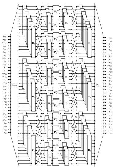
4. Evaluation of Computational Complexity

We will now calculate how many multiplications and additions of real numbers are required for the implementation of the new algorithm and will compare this with the number of operations required both for direct computation of matrix-vector products in Equation (1) and for implementing our previous algorithm [25]. The number of real multiplications required using the new algorithm is 192. Thus, using the proposed algorithm, the number of real multiplications needed to calculate the Kaluza number product is significantly reduced. The number of real additions required using our algorithm is 384. We observe that the direct computation of the Kaluza number product requires 608 additions more than the proposed algorithm. Thus, our proposed algorithm saves 832 multiplications and 960 additions of real numbers compared with the direct method. Thus, the total number of arithmetic operations for the proposed algorithm is approximately 71.4% less than that of the direct computation. The previously proposed algorithm [25] calculates the same result using 512 multiplications and 576 additions of real numbers. Thus, our proposed algorithm saves 62.5% of multiplications and 33.3% of additions of real numbers compared with our previous algorithm. Hence, the total number of arithmetic operations for the new proposed algorithm is approximately 47% less than that of our previous algorithm.

5. Conclusions

We presented a new effective algorithm for calculating the product of two Kaluza numbers. The use of this algorithm reduces the computational complexity of multiplications of Kaluza numbers, thus reducing implementation complexity and leading to a high-speed resource-effective architecture suitable for parallel implementation on VLSI platforms. Additionally, we note that the total number of arithmetic operations in the new algorithm is less than the total number of operations in the compared algorithms. Therefore, the proposed algorithm is better than the compared algorithms, even in terms of its software implementation on a general-purpose computer.

The proposed algorithm can be used in metacognitive neural networks using Kaluza numbers for data representation and processing. The effect in this case is achieved by using non-commutative finite groups based on the properties of the hypercomplex algebra [24]. When using the Kaluza number, in this case, the rule for generating the elements of the group will be set, as well as the rule for performing the group operation of multiplication. Such a system can contain two components: a neural network based on Kaluza numbers, which represents a cognitive component, and a metacognitive component, which serves to self-regulate the learning algorithm. At each stage, the metacognitive component will decide how and when the learning takes place. The algorithm removes unnecessary samples and keeps only those that are used. This decision will be determined by the magnitude and 31 phases of the Kaluza number. However, these matters are beyond the scope of this article and require more detailed research.

References

1. Kantor, I.L.; Solodovnikov, A.S. Hypercomplex Numbers: An Elementary Introduction to Algebras; Springer: Berlin/Heidelberg, Germany, 1989. [Google Scholar]
2. Alfsmann, D. On families of 2N-dimensional hypercomplex algebras suitable for digital signal processing. In Proceedings of the 2006 14th European Signal Processing Conference, Florence, Italy, 4–8 September 2006; pp. 1–4. [Google Scholar]
3. Alfsmann, D.; Göckler, H.G.; Sangwine, S.J.; Ell, T.A. Hypercomplex algebras in digital signal processing: Benefits and drawbacks. In Proceedings of the 2007 15th European Signal Processing Conference, Poznan, Poland, 3–7 September 2007; pp. 1322–1326. [Google Scholar]
4. Bayro-Corrochano, E. Multi-resolution image analysis using the quaternion wavelet transform. Numer. Algorithms 2005, 39, 35–55. [Google Scholar] [CrossRef]
5. Belfiore, J.C.; Rekaya, G. Quaternionic lattices for space-time coding. In Proceedings of the 2003 IEEE Information Theory Workshop (Cat. No. 03EX674), Paris, France, 31 March–4 April 2003; pp. 267–270. [Google Scholar]
6. Bulow, T.; Sommer, G. Hypercomplex signals-a novel extension of the analytic signal to the multidimensional case. IEEE Trans. Signal Process. 2001, 49, 2844–2852. [Google Scholar] [CrossRef] [Green Version]
7. Calderbank, R.; Das, S.; Al-Dhahir, N.; Diggavi, S. Construction and analysis of a new quaternionic space-time code for 4 transmit antennas. Commun. Inf. Syst. 2005, 5, 97–122. [Google Scholar]
8. Ertuğ, Ö. Communication over Hypercomplex Kähler Manifolds: Capacity of Multidimensional-MIMO Channels. Wirel. Person. Commun. 2007, 41, 155–168. [Google Scholar] [CrossRef]
9. Le Bihan, N.; Sangwine, S. Hypercomplex analytic signals: Extension of the analytic signal concept to complex signals. In Proceedings of the 15th European Signal Processing Conference (EUSIPCO-2007), Poznan, Poland, 3–7 September 2007; p. A5P–H. [Google Scholar]
10. Moxey, E.C.; Sangwine, S.J.; Ell, T.A. Hypercomplex correlation techniques for vector images. IEEE Trans. Signal Process. 2003, 51, 1941–1953. [Google Scholar] [CrossRef]
11. Comminiello, D.; Lella, M.; Scardapane, S.; Uncini, A. Quaternion convolutional neural networks for detection and localization of 3d sound events. In Proceedings of the ICASSP 2019–2019 IEEE International Conference on Acoustics, Speech and Signal Processing (ICASSP), Brighton, UK, 12–17 May 2019; pp. 8533–8537. [Google Scholar]
12. de Castro, F.Z.; Valle, M.E. A broad class of discrete-time hypercomplex-valued Hopfield neural networks. Neural Netw. 2020, 122, 54–67. [Google Scholar] [CrossRef] [Green Version]
13. Gaudet, C.J.; Maida, A.S. Deep quaternion networks. In Proceedings of the 2018 International Joint Conference on Neural Networks (IJCNN), Rio de Janeiro, Brazil, 8–13 July 2018; pp. 1–8. [Google Scholar]
14. Isokawa, T.; Kusakabe, T.; Matsui, N.; Peper, F. Quaternion neural network and its application. In Proceedings of the International Conference on Knowledge-Based and Intelligent Information and Engineering Systems, Oxford, UK, 3–5 September 2003; Springer: Berlin/Heidelberg, Germany, 2003; pp. 318–324. [Google Scholar]
15. Liu, Y.; Zheng, Y.; Lu, J.; Cao, J.; Rutkowski, L. Constrained quaternion-variable convex optimization: A quaternion-valued recurrent neural network approach. IEEE Trans. Neural Netw. Learn. Syst. 2019, 31, 1022–1035. [Google Scholar] [CrossRef]
16. Parcollet, T.; Morchid, M.; Linarès, G. A survey of quaternion neural networks. Artif. Intell. Rev. 2020, 53, 2957–2982. [Google Scholar] [CrossRef]
17. Saoud, L.S.; Ghorbani, R.; Rahmoune, F. Cognitive quaternion valued neural network and some applications. Neurocomputing 2017, 221, 85–93. [Google Scholar] [CrossRef]
18. Saoud, L.S.; Ghorbani, R. Metacognitive octonion-valued neural networks as they relate to time series analysis. IEEE Trans. Neural Netw. Learn. Syst. 2019, 31, 539–548. [Google Scholar] [CrossRef] [PubMed]
19. Vecchi, R.; Scardapane, S.; Comminiello, D.; Uncini, A. Compressing deep-quaternion neural networks with targeted regularisation. CAAI Trans. Intell. Technol. 2020, 5, 172–176. [Google Scholar] [CrossRef]
20. Vieira, G.; Valle, M.E. A General Framework for Hypercomplex-valued Extreme Learning Machines. arXiv 2021, arXiv:2101.06166. [Google Scholar]
21. Wu, J.; Xu, L.; Wu, F.; Kong, Y.; Senhadji, L.; Shu, H. Deep octonion networks. Neurocomputing 2020, 397, 179–191. [Google Scholar] [CrossRef]
22. Zhu, X.; Xu, Y.; Xu, H.; Chen, C. Quaternion convolutional neural networks. In Proceedings of the European Conference on Computer Vision (ECCV), Munich, Germany, 8–14 September 2018; pp. 631–647. [Google Scholar]
23. Bojesomo, A.; Liatsis, P.; Marzouqi, H.A. Traffic flow prediction using Deep Sedenion Networks. arXiv 2020, arXiv:2012.03874. [Google Scholar]
24. Saoud, L.S.; Al-Marzouqi, H. Metacognitive sedenion-valued neural network and its learning algorithm. IEEE Access 2020, 8, 144823–144838. [Google Scholar] [CrossRef]
25. Cariow, A.; Cariowa, G.; Łentek, R. An algorithm for multipication of Kaluza numbers. arXiv 2015, arXiv:1505.06425. [Google Scholar]
26. Silvestrov, V.V. Number Systems. Soros Educ. J. 1998, 8, 121–127. [Google Scholar]
27. Ţariov, A. Algorithmic Aspects of Computing Rationalization in Digital Signal Processing. (Algorytmiczne Aspekty Racjonalizacji Obliczeń w Cyfrowym Przetwarzaniu Sygnałów); West Pomeranian University Press: Szczecin, Poland, 2012. (In Polish) [Google Scholar]
28. Ţariov, A. Strategies for the synthesis of fast algorithms for the computation of the matrix-vector products. J. Signal Process. Theory Appl. 2014, 3, 1–19. [Google Scholar]