Article

Production Planning Problem of a Two-Level Supply Chain with Production-Time-Dependent Products

1
Department of Industrial and Management Engineering, Dong-A University, Busan 49315, Korea
2
Division of Business Administration & Accounting, Kangwon National University, Chuncheon-si 24341, Korea
3
Department of Business Administration, Kongju National University, Gongju-si 32588, Korea
*
Authors to whom correspondence should be addressed.
Appl. Sci. 2021, 11(20), 9687; https://doi.org/10.3390/app11209687
Submission received: 3 September 2021 / Revised: 13 October 2021 / Accepted: 14 October 2021 / Published: 17 October 2021
(This article belongs to the Special Issue Planning and Scheduling of Manufacturing Systems)

Abstract

:

Featured Application

Production planning problems with supply chains such as livestock, steel and chemical industries.

Abstract

This study considers a production planning problem with a two-level supply chain consisting of multiple suppliers and a manufacturing plant. Each supplier that consists of multiple production lines can produce several types of semi-finished products, and the manufacturing plant produces the finished products using the semi-finished products from the suppliers to meet dynamic demands. In the suppliers, different types of semi-finished products can be produced in the same batch, and products in the same batch can only be started simultaneously (at the same time) even if they complete at different times. The purpose of this study is to determine the selection of suppliers and their production lines for the production of semi-finished products for each period of a given planning horizon, and the objective is to minimize total costs associated with the supply chain during the whole planning horizon. To solve this problem, we suggest a mixed integer programming model and a heuristic algorithm. To verify performance of the algorithm, a series of tests are conducted on a number of instances, and the results are presented.

1. Introduction

This study considers a problem of production planning in a two-level supply chain consisting of multiple suppliers and a manufacturing plant. Each supplier that consists of multiple production lines can produce several types of semi-finished products and the manufacturing plant produces the finished products using the semi-finished products from the suppliers to meet dynamic demands. The planning manager of this supply chain selects suppliers to produce semi-finished products and determines the quantity of semi-finished products to be produced for each period to minimize total costs associated with the supply chain (the information of demand in each period is known in advance).
We focus on a case in which semi-finished products are produced by almost the same general process, but those products are sorted according to their production times. That is, the type of semi-finished product depends on the production time. In this paper, we assume that different types of semi-finished products can be produced in the same batch, and products in the same batch can only be started simultaneously (at the same time) even if they complete at different times. Such production characteristics (called production time-dependent products) can be easily found in food industries such as fermented foods, wines, and poultry. In the case of poultry farming industry, it has only been studied to analyze diseases and environmental issues [1,2], or to determine the location and size of livestock [3]. However, production management of the poultry industry is also one of the most important issues, but there is little research on this issue. Therefore, we focus on the production planning with consideration of characteristics of poultry farming.
In this industry, sizes (or weights) of the products are one of major attributes that distinguish the types of final products. In the suppliers, the size (weight) of the poultry may be the only distinguishing attribute if we do not consider exceptional cases like infection of diseases. In general, the size of poultry depends on the breeding time, and hence production plans for the semi-finished products at the suppliers are established considering the breeding time (or production time) of the semi-finished products. The production time-dependent products can also be found in other industries such as steel industry and chemical industry.
In the poultry industry, many companies own and operate manufacturing plants and many poultry farms together. In the concept of supply chains, the farms occupy the role of suppliers. However, the farms are not independent but are subordinate to headquarters. Therefore, the production plan of such suppliers depends on the manufacturer’s plan. Based on this situation, we consider a system in which one management unit controls all suppliers and a manufacturing plant. The management determines:
  • whether each supplier should be opened and operated in each period;
  • the total production quantities of the semi-finished product among candidate levels;
  • production quantities of each type of semi-finished product at the operated suppliers in each period.
When we determine suppliers to start production in each period, we also have to determine production quantity levels of the suppliers. For example, in real-world cases of poultry farms, there may be multiple numbers of production quantity levels depending on the number of production lines of a farm. That is, production quantity levels of farms are determined by the number of production lines to be operated to satisfy the quantity of products to be produced in each period. In other words, the farms may have to determine production quantity levels of semi-finished products in each period. We call this problem as the production planning problem with discrete production quantity levels for production-time-dependent products (FLPP-VC).
As mentioned above, the FLPP-VC determines production quantity levels in each period as a normal production planning problem. However, in each period, not every supplier starts its setup operation for processing a production batch. Therefore, we have to determine not only the production quantity, but also suppliers to be operated. Focusing on the determination in each period, the considered problem becomes the special case of a typical facility location problem (FLP). Both problems deal with selecting locations of the facilities to be operated among possible (candidate) facilities to satisfy the demand. Additionally, in general, these decisions are handled by the central manager of department, taking into account the entire systems. However, in a typical FLP, the locations of facilities are decided at the beginning of the planning horizon and the locations are fixed throughout the entire period, whereas the decisions on suppliers’ operations in the FLPP-VC can be changed during the planning horizon.
The studies of FLPP-VC are very rare, while FLPs have been studied by many researchers. Thus, we categorized and reviewed the variants of FLPs into four parts: uncapacitated FLP, capacitated FLP, dynamic FLP, and FLP determining capacities. For an uncapacitated facility location problem (UFLP), a branch-and-bound algorithm (B&B) was proposed in [4]. Additionally, for capacitated facility location problems (CFLPs), various algorithms were devised, including B&B [5,6], genetic algorithms [7,8,9,10], and Lagrangian relaxation based heuristic algorithms [11,12,13,14].
The dynamic facility location problem (DFLP), which is an FLP with multi-period dynamic demands, is very similar to our problem (FLPP-VC). However, like a typical FLP, the locations of the facilities in the DFLP are determined once at the beginning and not changed, even if it can worsen the overall efficiency of the supply chain for the entire planning period. Additionally, the semi-finished products inventory is not allowed in FLPP-VC, while DFLP can have positive inventory. For the DFLP, dynamic programming algorithms were developed in [15,16,17], while a simulated annealing was developed in [18] and an MIP based heuristic algorithm in [19]. In addition, an optimal solution algorithm was suggested in [20], considering a dual problem of the original DFLP. Additionally, ref. [21] studied an extended version of the problem considering setup, transportation, production costs and taxes (between two countries), and proposed a branch-and-bound algorithm, while [22] studied the problem considering relocation of facilities for the planning horizon and propose heuristics based on Bender’s decomposition and Lagrangian relaxation method. In their model, the opening and closing of the facilities are determined in each period but opening decisions for each facility can be done only once in the planning horizon. Ref. [23] considered a multi-period facility location problem with two different classes of customers, depending on the tolerance of delayed delivery. Ref. [24] proposed heuristic algorithms for dynamic facility location problems consisting of determining locations and sizes of facilities. Several extensions of the DFLP are also found, such as considering multi-commodities [25,26] and time restrictions for deliveries [27]. Furthermore, many heuristics and exact methods have been studied to solve the discrete multi-period facilities location problem, for example in [28,29,30,31,32].
In the considered problem, capacities of facilities can be changed. There have been very few previous studies, if any, in which changeable capacity levels were considered. However, the FLPs with determining capacities of suppliers have been considered in several studies. Among them, refs. [33,34,35,36,37] consider models in which at most one capacity level can be selected among a set of possibilities. Additionally, there are some studies on FLPs in which expansion of capacities is considered [38,39,40,41,42]. On the other hand, the production-time-dependent products dealt with in this paper have just been introduced in [43], and [44] studied a production planning problem of a two-level supply chain with production-time-dependent products considering outsourcing. These two studies consider that each supplier has only one production line, whereas this study considers multiple production lines in each supplier. Note that, in practice, a facility with multiple production lines opens the appropriate number of lines, not all lines.
Finally, we reviewed several papers related to centralized supply chains that are controlled by a central managerial department (or manager): ref. [45] developed a model to design a centralized supply chain network in markets under deterministic price-depended demands and with a rival chain present; ref. [46] analyzed and compared centralized and decentralized model predictive control strategies to control inventory positions and to reduce the bullwhip effect in a benchmark four-echelon supply chain; ref. [47] investigated the supply chain scenarios for their relevant performance at the conceptual design stage and showed that the centralized supply chain scenario demonstrates superiority in cost performance; ref. [48] presented a mathematical model to plan logistics activities in a forest products supply chain; ref. [49] analyzed control policies for a centralized two-stage supply chain with subcontractors at each stage a number of numerical results show the impact of variations in certain system parameters on file optimal control parameters and the corresponding profit; and ref. [50] explored the impact of misplaced inventory on a centralized two-level supply chain, which consists of a risk-neutral supplier and a risk-averse retailer.
The main contributions of this paper are as follows. To the best of our knowledge, this study is the first attempt to solve a production planning problem that needs to determine the location of facilities (suppliers) with multiple production lines in each period and the quantities of production-time-dependent products to be produced in each supplier. For the problem, we propose a mixed-integer linear programming (MILP) and a heuristic algorithm, considering variable capacity levels for production-time-dependent products with dynamic demands in a two-level supply chain. The heuristic algorithm consists of two steps: determining locations of facilities and then determining capacities of the facilities, i.e., determining which suppliers should be operated in each period, and the quantity produced for each type of semi-finished product from the supplier (selected for operating in each period).
This paper is organized as follows. In Section 2, we present the MILP and explain the problem in detail, and then we introduce a heuristic algorithm in Section 3. In Section 4, to evaluate the performance of our proposed algorithm, computational experiments are performed, and the results are reported. Finally, we conclude this paper with a short summary and discuss possible extensions of our study in Section 5.

2. Problem Description

This study considers a problem of production planning for the production-time-dependent products in a two-level supply chain consisting of multiple suppliers and a manufacturing plant. Each supplier has an upper limited capacity for production quantity which can be produced simultaneously at the same batch. However, it is assumed that the manufacturing plant is uncapacitated, that is, the plant can satisfy all demands of external customers. In a poultry industry, the production process of a manufacturer is simple and automated, such as packaging or cutting. Additionally, in general, the capacity of manufacturer is relatively larger than those of the suppliers. Thus, it is sufficient to consider only the capacities of suppliers for solving the real problem. To establish a production plan for the considered supply chain, a planning manager determines which suppliers start to produce semi-finished products in each period, capacities of the selected suppliers, and production quantities of each semi-finished product type at each supplier. The results of the planning are quantities of raw materials to be input into the suppliers for production of the semi-finished products.
As mentioned in the previous section, the considered problem is motivated from a poultry farming industry in Korea. Thus, this study makes the following assumptions based on the situation of the poultry farming industry.
  • The supply chain consists of multiple suppliers and a manufacturing plant;
  • Locations of the manufacturing plant and the (candidate) suppliers are pre-determined and given;
  • The suppliers produce several types of semi-finished products, and different semi-finished products may be produced at the same production line of a supplier. Note that we need to decide suppliers, product lines, and product types to produce, respectively;
  • If two or more types of semi-finished products are to be produced at the same supplier, they should be started simultaneously;
  • In a supplier, a new batch cannot be started while a batch is being produced;
  • A setup operation is needed (for cleaning and maintenance of a production line) at each supplier before each production run of a batch;
  • The capacity levels of production lines of each supplier and setup cost for each level are known and fixed;
  • Capacity of each supplier is equal to the sum of capacity levels of production lines in the supplier;
  • The demand for each product type in each period may vary by period and is known in advance;
  • There is no shortage of raw material for the semi-finished products;
  • There is no defective in the production process at the suppliers. Hence, the input and the output quantities at a supplier are the same;
  • All suppliers are ready to start production at the beginning (starting) of the planning horizon. In addition, there is no need for a setup operation for the first batch of the planning horizon;
  • The transportation time is negligibly short (compared to a period);
  • Only one production line can be selected and operated for a supplier at each operating period;
  • Production quantity of operated production line in a supplier to be operated in each period is equal to the capacity of the operated production line.
For a clearer description of the problem, we develop a mixed integer programming formulation. We use this formulation to find an optimal solution for this problem using a commercial integer programming solver in the computational experiments.
The following notation is used throughout the paper.

2.1. Indices and Parameters

i 
index for suppliers (i = 1,…, I)
l 
index for semi-finished product types (l = 1,…, L)
t 
index for time periods (t = 1,…,T)
j 
index for production lines (j = 1,…,J)
p l
production time (in the number of time periods) of semi-finished product type l at the suppliers
S i j U
setup cost for each batch at supplier i with production line j
K i j
capacity of production line j at supplier i
D l t
demand quantity (at the manufacturing plant) of semi-finished product type l in period t
C i l P
production cost per one unit of semi-finished product type l at supplier i
C i l T
transportation cost per one unit of semi-finished product type l from supplier i to the manufacturing plant
M 
a very large (positive) number

2.2. Decision Variables

Q i j l t
production quantity of semi-finished product type l, the quantity that is being processed, at production line j in supplier i on period t
Y i j l t
= 1 if production line j of supplier i starts processing semi-finished product l in period t, and 0 otherwise
Z i j t
= 1 if production line j of supplier i starts producing semi-finished products in period t, and 0 otherwise
Now, we give a mixed integer programming formulation for our problem below.
[ P ]   Minimize i j t S i j U Z i j t + i j l t ( C i l P + C i l T ) Q i j l t
subject   to i j Q i j l t D l , t + p l              l ,   t
l Q i j l t = K i j · Z i j t              i ,   j ,   t
j Z i j t 1              i , t
l Y i j l t L · Z i j t            t = 1 , ,   T p l ,     i ,   j ,   l
t = t + 1 t + p l Z i j t M · ( 1 Y i j l t )            t = 1 , ,   T p l ,     i ,   j ,   l
Q i j l t M · Y i j l t              i ,   j ,   l ,   t
Q i j l t 0              i ,   j ,   l ,   t
Y i j l t , Z i j t { 0 , 1 }              i ,   j ,   l ,   t
The objective function (1) is to minimize the total costs incurred in the supply chain, including setup costs of suppliers to start production, production costs at the suppliers, and transportation costs from suppliers to the manufacturing plant. Constraint (2) ensures demand is satisfied, i.e., the sum of production quantities of suppliers for each semi-finished product type is larger than demand. Constraint (3) ensures that the total production quantity is equal to the capacity of the operated production line of the supplier operated in each period. Constraint (4) ensures that only one production line can be selected and operated for a supplier at each operating period. Additionally, constraint (5) ensures that the selected production line can produce up to L types of products. This constraint defines relationship between Y i j l t and Z i j t . In addition, constraint (6) prevents a supplier from starting a new batch in the middle of processing a batch. Constraint (7) defines the relationships between Q i j l t and Y i j l t . Constraints (8) and (9) define the domain of decision variables.

3. Heuristic Algorithm

Since an uncapacitated facility location problem (UFLP) is known as NP-hard [51], our problem, FLPP-VC, is also NP-hard. Note that the UFLP is a special case of the FLPP-VC, that is, it is the case in which the capacities of the facilities are unlimited, demands of each product in all periods are the same, and suppliers produce a single product. Since it may take an excessive amount of time to obtain optimal solutions of the FLPP-VC using a commercial solver even for small-size instances, we present a two-step heuristic algorithm in this paper.
First, to simplify the problem, we group the demands for semi-finished products (of the same type or different types) based on the start time to produce the semi-finished products for satisfying the demand. That is, a demand group for period t is the set of demands for all semi-finished product types that must be started at period t in order for the supplier’s production to meet the demands on time. Before explaining the heuristic in detail, an additional notation is provided.
i 
for suppliers (i = 1,…, I)
l 
index for semi-finished product
D ˜ t
total demand quantity of demand group t, i.e., the sum of demand quantities of semi-finished products for which the production should be started in period t to meet their demand
C ¯ i p
average of production costs of semi-finished product types produced at supplier i, l = 1 L C i l p / L
C ¯ i t
average of transportation costs of semi-finished product types produced at supplier i, l = 1 L C i l t / L
E t av
set of suppliers that are available (to start production) in period t, those have been set up at the beginning of period t for production of semi-finished products
E t s t
set of suppliers that are to start production in period t
Zijt 
= 1 if i E t s t , i.e., if supplier i with production line j is selected to start production in period t, and 0 otherwise
To develop the two-step heuristic algorithm, we decompose the considered problem into two parts, and these are solved in each of the two steps, respectively. In the first step, we select suppliers that produce semi-finished products in each period and determine a production line of the selected suppliers. This decision made at the first step is related to the allocation of the suppliers to each period. Given the selected suppliers in each period, the second step is to determine the production quantity of each semi-finished product type at each of the selected suppliers. However, it may take an excessive amount of time if we consider demands for all semi-finished product types in all periods individually. Therefore, we use the concept of the demand group defined above.
In the first step, the following integer program is used for the selection decisions for period t where t = 1, 2, …, T. Here, we use a new cost term, V i j = S i j U + ( C ¯ i p + C ¯ i t ) K i j , which represents the setup, production, and transportation costs associated with supplier i of production line j.
[ IP t ]   Minimize i E t a v j V i j · Z i j
subject   to i E t a v K i j · Z i j t D ˜ t              j
j Z i j t 1              i
Z i j t { 0 , 1 }              i ,   j
By the objective function, the sum of the operation costs at the suppliers in period t is minimized. Constraint (11) ensures that the sum of capacity of production lines of the selected suppliers in E t a v can satisfy the demand quantity of the demand group of period t. Therefore, by using [IPt], we can select suppliers to satisfy the demand in period t with the minimum cost.
Even though [IPt] is based on the simplified demand groups, it is not easy to find the optimal solution of [IPt]. As an alternative, we suggest a heuristic algorithm to select suppliers and determine their production line to produce semi-finished products. In each period, we first select a supplier with the minimum operating cost (Vit) among those in E t a v and add the selected supplier into E t s t . If the demand quantity of the demand group is not satisfied by the selected supplier, other suppliers are selected one by one with the same method until the demand is satisfied by the capacity levels of the selected suppliers.
When suppliers are selected for demand group of period 1, all suppliers with all (candidate) production lines are available, that is, all suppliers are in E 1 a v . If suppler i with production line j is selected in period 1, it is included in the set of selected suppliers ( E 1 s t ) and is not considered for being selected until the production of a batch is completed. By updating E t a v for the subsequent periods, we can solve [IPt] and obtain E t s t for ∀t = 1, 2, …, T.
Once suppliers are allocated to each period, that is, suppliers to be opened (or operated) in each period and their production line for producing are determined, the subproblem of determining production quantities of each supplier can be defined, and it is formulated as the following linear program.
[ LP ]   Minimize            i E t s t j l ( C i l p + C i l t ) Q i j l t + i E t s t j S i j U · Z i j t
subject   to            i E t s t j Q i j l t D l , t + p l              l
l Q i j l t = K i j · Z i j t              i E t s t ,   j
Q i j l t 0              i E t s t ,   j ,   l
Solution values of the second term of the objective function (14) are given from the solutions of (IPt). Constraints (15), (16), and (17) correspond to (2), (3), and (8), respectively. Constraint (15) ensures that the sum of production quantities of suppliers for each semi-finished product type in period t have to satisfy the demand in period t. Constraints (16) ensures that the capacity of the operated production line of the supplier operated in period t is equal to the total production quantity in period t. Note that only the suppliers selected to produce semi-finished products, i.e., suppliers i such that i E t s t , are considered in [LP], and hence there are much fewer constraints to be considered. In our solution procedure, [LP] is solved with a commercial programming solver for linear programming.
By applying the above two steps sequentially, we can obtain a feasible, and possibly a good solution of FLPP-VC. The overall procedure of the heuristic can be summarized as follows.
Procedure 1. (Two-step heuristic for FLPP-VC)
Step 0
Set E 0 a v   = {1, 2, …, I}, E 1 s t = ∅, t=1, and TC* = ∞. Compute D ˜ t for t = 1,…, T, and Vij for i = 1,…, I and j = 1,…, J. Let t = 1.
Step 1
If there are suppliers with D ˜ t < K i j , select a supplier with the smallest value of V i j among them; otherwise, select a supplier and its production line with the smallest V i j among suppliers in E t a v . Update E t s t and E t a v , and let D ˜ t D ˜ t K i j .
Step 2
If D ˜ t > 0 , go to Step 1. Otherwise ( D ˜ t 0 ), if t = T, go to Step 3; otherwise, let tt + 1 and go to Step 1.
Step 3
Solve the linear program, [LP], defined by the solution of Step 1 (with a commercial LP solver), and stop.

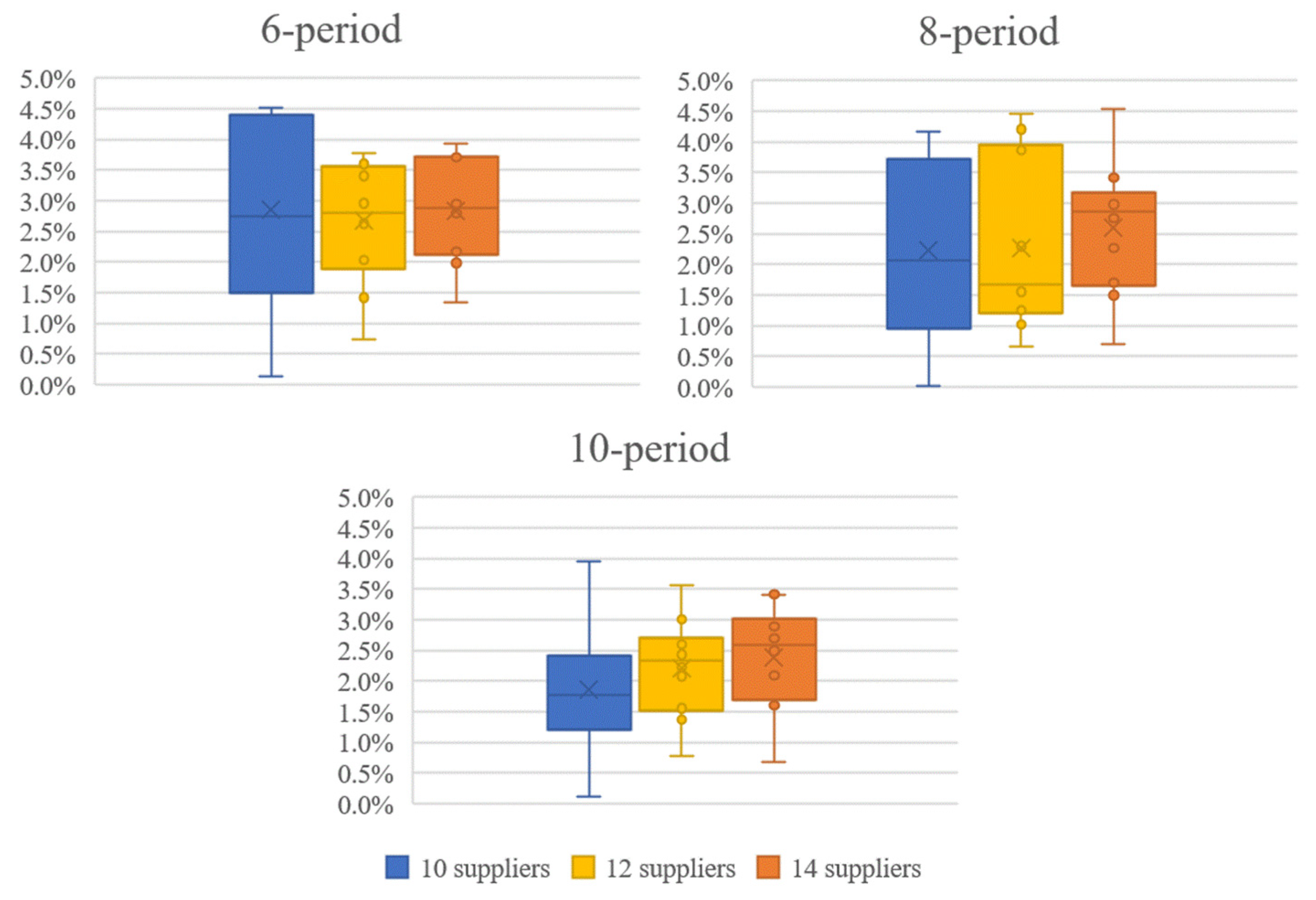
4. Computational Experiments

In this paper, we evaluated the suggested algorithm through computational experiments on a number of problem instances. These problem instances were generated randomly based on real information from a poultry company in Korea. Three levels of the number of supplies (I = 10, 12, and 14) and three levels of the length of planning horizon (T = 6, 8, and 10) were considered. For the nine combinations of (I and T), 10 instances were generated (totally 90 instances). Based on the information from the poultry company, we considered three types of semi-finished products with different processing time (L = 3, 4, and 5), and the numbers of candidate production line are three for all suppliers (J = 3). Other data were generated as follows. Here, U(a, b) represents the discrete uniform distribution with range [a, b].
  • Demand was generated from U(500, 800) for all types of product at each period;
  • The capacities of the three production lines at a supplier were generated from U(100, 200), U(200, 300), and U(300, 400), and setup costs for these production lines were generated from U(500, 1000), U(1000, 1500), and U(1500, 2000), respectively;
  • The production cost of each type of semi-finished products of a supplier were generated from U(10, 15), U(20, 25), and U(30, 35). The transportation costs between a supplier and the manufacturing plants were generated from U(5, 10), U(10, 15), and U(15, 20) for semi-finished product types 1, 2, and 3, respectively.
The heuristic algorithm was coded in Java programming language, and a commercial solver CPLEX was used for the linear and integer programs. We set the computation time limit to 15,000 s for an instance to prevent prolonged execution time. All tests were operated on a personal computer with AMD Phenom II (3.0-GHz) and 3 GB RAM.
Results of the test are given in Table 1, Table 2 and Table 3, which show solution values of the heuristic and CPLEX, CPU times, and percentage errors of the heuristic solutions from the solutions (or lower bounds) obtained by CPLEX. As can be seen from Table 1, for only 4 instances (with ten suppliers) out of 30 instances, the percentage errors were larger than 4%. Table 2 and Table 3 show similar results for larger instances. These results demonstrate the performance of the suggested heuristic algorithm that can give reasonably good solutions regardless of the length of the planning horizon. Additionally, the heuristic shows almost the same performance regardless of the number of the suppliers. The overall average percentage error (PE, %) of the 90 instances was 2.43%. Figure 1 shows the summary of the results of percentage errors according to different number of periods and suppliers. As shown in the figure, we could not find significant correlation between problem size and the percentage error.
For the 6-period instances, CPLEX required 15.31 s on average, while the suggested heuristic required only 0.01 s. In these instances, CPU time for both methods may look reasonable. However, as the length of the planning horizon increased, CPU times for CPLEX increased significantly, longer than one hour. On the other hand, the suggested heuristic found good solutions in a very short time. In the 10-period instances, which reflect practical situations, many instances failed to give an optimal solution by CPLEX within the time limit (15,000 s). In fact, we performed tests on instances of larger sizes (I > 14, T > 10), but none of these instances were solved by CPLEX within the time limit. In real situations, in which demand forecasts may be changed frequently, the problem may have to be solved accordingly, and even one hour for the solution of the planning problem may be considered too long.
In real situations in poultry farming companies, they have to establish a weekly production plan within one or two hours, but it may be required to modify or re-make due to changed forecast values. Therefore, the heuristic algorithm can be effectively used for such situations, because it gives reasonably good solutions within a very short computation time. Additionally, for longer-term planning with T > 10, which a company needs to prepare for demand fluctuations, the suggested heuristic may be more appropriate than CPLEX. Moreover, the results or solutions for the problem can be used for managerial decision by evaluating efficiency of the supply chain with selected production line. For example, if the production quantity is smaller than demand, they can change the production line of suppliers. On the other hands, if the production quantity is larger than demand, the company can reduce the number of suppliers to be operated. In other words, the proposed heuristic can also be used for design of the supply chain.

5. Discussion and Conclusions

This study investigated a planning problem for production in a two-level supply chain in which there are multiple suppliers with different capacity levels and a single manufacturing plant with dynamic demands for production-time-dependent products. This problem is to select suppliers to produce semi-finished products and to determine production quantities to be produced at the determined suppliers, in each period during the planning horizon. For the problem, a mixed integer programming model is provided, and a heuristic algorithm is also suggested to obtain good solutions quickly. In the heuristic, the problem is solved in two steps, selection of suppliers to be operated and their production line and then determination of production quantities at the suppliers. The two decisions are made sequentially with a heuristic method and a commercial LP solver.
This study can be the basis for research on production management of poultry and livestock industries. In addition, the study is highly expandable because the characteristics of production-time dependent can be found in various fields such as steel, fermented food, liquor, and chemical industries. This research can be extended in several ways. Since this study is the first attempt to consider a problem dealt with a design of supply chain and a production planning for the production-time-dependent products simultaneously, the considered model can be applied to a supply chain with similar characteristics. In addition, one may need to case involving determination of the locations of suppliers and manufacturing plants to design a supply chain. Also, research on the problem of limited capacity of the manufacturer can be studied and applied to various industries. Then, in the future, we can consider the problem in which the manufacturer and suppliers are not under the control of the one company unit.

Author Contributions

Conceptualization, J.-H.H., and B.J.; methodology, J.-H.H., J.-Y.L., and B.J.; software, J.-H.H., and J.-Y.L.; validation, J.-H.H., J.-Y.L., and B.J.; formal analysis, J.-H.H.; investigation, J.-H.H.; resources, J.-H.H.; data curation, J.-H.H., and J.-Y.L.; writing—original draft preparation, J.-H.H., J.-Y.L., and B.J.; writing—review and editing, J.-H.H., J.-Y.L., and B.J.; visualization, J.-Y.L.; supervision, B.J.; project administration, J.-H.H.; funding acquisition, J.-H.H. All authors have read and agreed to the published version of the manuscript.

Funding

This work was supported by the Dong-A University research fund.

Data Availability Statement

The data used to support the findings of this study are available from the corresponding author upon request.

Conflicts of Interest

The authors declare no conflict of interest.

References

  1. Mekonnen, M.; Hoekstra, A. A global assessment of the water footprint of farm animal products. Ecosystems 2012, 15, 401–415. [Google Scholar] [CrossRef] [Green Version]
  2. Mottet, A.; Tempio, G. Global poultry production: Current state and future outlook and challenges. World Poult. Sci. J. 2017, 73, 245–256. [Google Scholar] [CrossRef] [Green Version]
  3. Fischer, G.; Ermolieva, T.; Ermoliev, Y.; van Velthuizen, H. Livestock production planning under environmental risks and uncertainties. J. Syst. Sci. Syst. Eng. 2006, 15, 399–418. [Google Scholar] [CrossRef]
  4. Erlenkotter, D. A dual-based procedure for uncapacitated facility location. Oper. Res. 1978, 26, 992–1009. [Google Scholar] [CrossRef]
  5. Neebe, A.W.; Rao, M.R. An algorithm for the fixed-charge assigning users to sources problem. J. Oper. Res. Soc. 1983, 34, 1107–1113. [Google Scholar] [CrossRef]
  6. Yang, Z.; Chu, F.; Chen, H. A cut-and-solve based algorithm for the single-source capacitated facility location problem. Eur. J. Oper. Res. 2012, 221, 521–532. [Google Scholar] [CrossRef]
  7. Atabaki, M.S.; Mohammadi, M.; Naderi, B. Hybrid genetic algorithm and invasive weed optimization via priority based encoding for location-allocation decisions in a three-stage supply chain. Aisa Pac. J. Oper. Res. 2017, 34, 1750008. [Google Scholar] [CrossRef]
  8. Suzuki, A.; Yamamoto, H. Solving facility rearrangement problem using a genetic algorithm and a heuristic local search. Ind. Eng. Manag. Syst. 2012, 11, 170–175. [Google Scholar] [CrossRef] [Green Version]
  9. Wang, X.; Sun, X.; Fang, Y. Genetic algorithm solution for multi-period two-echelon integrated competitive/uncompetitive facility location problem. Aisa Pac. J. Oper. Res. 2008, 25, 33–56. [Google Scholar] [CrossRef]
  10. Yang, F.-C.; Kao, S.-L. An agent gaming and genetic algorithm hybrid method for factory location setting and factory/supplier selection problem. Ind. Eng. Manag. Syst. 2009, 8, 228–238. [Google Scholar]
  11. Christofides, N.; Beasley, J.E. Extensions to a Lagrangian relaxation approach for the capacitated warehouse location problem. Eur. J. Oper. Res. 1983, 12, 19–28. [Google Scholar] [CrossRef]
  12. Barcelo, J.; Casanovas, J. A heuristic Lagrangian algorithm for the capacitated plant location problem. Eur. J. Oper. Res. 1984, 15, 212–226. [Google Scholar] [CrossRef]
  13. Klincewicz, J.G.; Luss, H. A lagrangian relaxation heuristic for capacitated facility location with single-source constraints. J. Oper. Res. Soc. 1986, 37, 495–500. [Google Scholar] [CrossRef]
  14. Kim, C.-Y.; Choi, G.-H. Adaptive mean value cross decomposition algorithms for capacitated facility location problems. J. Korea Inst. Ind. Eng. 2011, 37, 124–131. [Google Scholar] [CrossRef]
  15. Wesolowsky, G.O. Dynamic facility location. Manag. Sci. 1973, 19, 1241–1248. [Google Scholar] [CrossRef]
  16. Wesolowsky, G.O.; Truscott, W.G. The multiperiod location-allocation problem with relocation of facilities. Manag. Sci. 1975, 22, 57–65. [Google Scholar] [CrossRef]
  17. Sweeney, D.J.; Tatham, R.L. An improved long-run model for multiple warehouse location. Manag. Sci. 1976, 22, 748–758. [Google Scholar] [CrossRef] [Green Version]
  18. Chardaire, P.; Sutter, A.; Costa, M.C. Solving the dynamic facility location problem. Networks 1996, 28, 117–124. [Google Scholar] [CrossRef]
  19. Canel, C.; Khumawala, B.M. International facilities location: A heuristic procedure for the dynamic uncapacitated problem. Int. J. Prod. Res. 2001, 39, 3975–4000. [Google Scholar] [CrossRef]
  20. Roy, T.J.V.; Erlenkotter, D. A dual-based procedure for dynamic facility location. Manag. Sci. 1982, 28, 1091–1105. [Google Scholar] [CrossRef] [Green Version]
  21. Canel, C.; Khumawala, B. Multi-period international facilities location: An algorithm and application. Int. J. Prod. Res. 1997, 35, 1897–1910. [Google Scholar] [CrossRef]
  22. Torres-Soto, J.; Uster, H. Dynamic-demand capacitated facility location problems with and without relocation. Int. J. Prod. Res. 2011, 49, 3979–4005. [Google Scholar] [CrossRef]
  23. Sauvey, C.; Melo, T.; Correia, I. Heuristics for a multi-period facility location problem with delayed demand satisfaction. Comput. Ind. Eng. 2020, 139, 106171. [Google Scholar] [CrossRef]
  24. Silva, A.; Aloise, D.; Coelho, L.; Rocha, C. Heuristics for the dynamic facility location problem with modular capacities. Eur. J. Oper. Res. 2021, 290, 435–452. [Google Scholar] [CrossRef]
  25. Jena, S.; Cordeau, J.; Gendron, B. Solving a dynamic facility location problem with partial closing and reopening. Comput. Oper. Res. 2016, 67, 143–154. [Google Scholar] [CrossRef]
  26. Correia, I.; Melo, T. A multi-period facility location problem with modular capacity adjustments and flexible demand fulfillment. Comput. Ind. Eng. 2017, 110, 307–321. [Google Scholar] [CrossRef]
  27. Jena, S.; Cordeau, J.; Gendron, B. Lagrangian heuristics for large-scale dynamic facility location with generalized modular capacities. INF J. Comput. 2017, 29, 388–404. [Google Scholar] [CrossRef]
  28. Boujelben, M.K.; Gicquel, C.; Minoux, M. A MILP model and heuristic approach for facility location under multiple operational constraints. Comput. Ind. Eng. 2016, 98, 446–461. [Google Scholar] [CrossRef] [Green Version]
  29. Marufuzzaman, M.; Gedik, R.; Roni, M. A Benders based rolling horizon algorithm for a dynamic facility location problem. Comput. Ind. Eng. 2016, 98, 462–469. [Google Scholar] [CrossRef] [Green Version]
  30. Castro, J.; Nasini, S.; Saldanha-da-Gama, F. A cutting-plane approach for large-scale capacitated multi-period facility location using a specialized interior-point method. Math. Program. 2017, 163, 411–444. [Google Scholar] [CrossRef] [Green Version]
  31. Dong, Y.K.; Wang, J.Y.; Chen, F.H.; Hu, Y.; Deng, Y. Location of facility based on simulated annealing and “ZKW” algorithms. Math. Probl. Eng. 2017, 2017, 4628501. [Google Scholar] [CrossRef] [Green Version]
  32. Rahmani, A.; Yousefikhoshbakht, M. A benders decomposition method for dynamic facility location in integrated closed chain problem. Math. Probl. Eng. 2021, 2021, 6684029. [Google Scholar] [CrossRef]
  33. Mazzola, J.B.; Neebe, A.W. Lagrangian-relaxation-based solution procedures for a multiproduct capacitated facility location problem with choice of facility type. Eur. J. Oper. Res. 1999, 115, 285–299. [Google Scholar] [CrossRef]
  34. Amiri, A. Designing a distribution network in a supply chain system: Formulation and efficient solution procedure. Eur. J. Oper. Res. 2006, 171, 567–576. [Google Scholar] [CrossRef]
  35. Elhedhli, S.; Gzara, F. Integrated design of supply chain networks with three echelons, multiple commodities and technology selection. IIE Trans. 2008, 40, 31–44. [Google Scholar] [CrossRef]
  36. Amrani, H.; Martel, A.; Zufferey, N.; Makeeva, P. A variable neighborhood search heuristic for the design of multicommodity production-distribution networks with alternative facility configurations. OR Spectr. 2011, 33, 989–1007. [Google Scholar] [CrossRef]
  37. Correia, I.; Melo, T.; Saldanha-da-Gama, F. Comparing classical performance measures for a multi-period, two-echelon supply chain network design problem with sizing decisions. Comput. Ind. Eng. 2013, 64, 366–380. [Google Scholar] [CrossRef] [Green Version]
  38. Shulman, A. An algorithm for solving dynamic capacitated plant location problems with discrete expansion sizes. Oper. Res. 1991, 39, 423–436. [Google Scholar] [CrossRef]
  39. Antunes, A.; Peeters, D. On solving complex multi-period location models using simulated annealing. Eur. J. Oper. Res. 2001, 130, 190–201. [Google Scholar] [CrossRef] [Green Version]
  40. Hugo, A.; Pistikopoulos, E. Environmentally conscious long-range planning and design of supply chain networks. J. Cleaner Prod. 2005, 13, 1471–1491. [Google Scholar] [CrossRef]
  41. Thanh, P.; Bostel, N.; Peton, O. A dynamic model for facility location in the design of complex supply chains. Int. J. Prod. Econ. 2008, 113, 678–693. [Google Scholar] [CrossRef]
  42. Thanh, P.; Peton, O.; Bostel, N. A linear relaxation-based heuristic approach for logistics network design. Comput. Ind. Eng. 2010, 59, 964–975. [Google Scholar] [CrossRef]
  43. Han, J.; Kim, Y. Design and operation of a two-level supply chain for production-time-dependent products using Lagrangian relaxation. Comput. Ind. Eng. 2016, 96, 118–125. [Google Scholar] [CrossRef]
  44. Han, J.; Lee, J.; Kim, Y. Production planning in a two-level supply chain for production-time-dependent products with dynamic demands. Comput. Ind. Eng. 2019, 135, 1–9. [Google Scholar] [CrossRef]
  45. Rezapour, S.; Farahani, R.Z. Strategic design of competing centralized supply chain networks for markets with deterministic demands. Adv. Eng. Softw. 2010, 41, 810–822. [Google Scholar] [CrossRef]
  46. Fu, D.F.; Ionescu, C.M.; Aghezzaf, E.H.; De Keyser, R. Decentralized and centralized model predictive control to reduce the bullwhip effect in supply chain management. Comput. Ind. Eng. 2014, 73, 21–31. [Google Scholar] [CrossRef]
  47. Chiu, M.C.; Kremer, G.E.O. An Investigation on Centralized and Decentralized Supply Chain Scenarios at the Product Design Stage to Increase Performance. IEEE Trans. Eng. Manag. 2014, 61, 114–128. [Google Scholar] [CrossRef]
  48. Alayet, C.; Lehoux, N.; Lebel, L.; Bouchard, M. Centralized supply chain planning model for multiple forest companies. INFOR 2016, 54, 171–191. [Google Scholar] [CrossRef]
  49. Saharidis, G.K.D.; Kouikoglou, V.S.; Dallery, Y. Centralized and decentralized control polices for a two-stage stochastic supply chain with subcontracting. Int. J. Prod. Econ. 2009, 117, 117–126. [Google Scholar] [CrossRef]
  50. Zhu, L.J.; Lee, C. Risk Analysis of a Two-Level Supply Chain Subject to Misplaced Inventory. Appl. Sci.-Basel 2017, 7, 676. [Google Scholar] [CrossRef] [Green Version]
  51. Cornuéjols, G.; Nemhauser, G.L.; Wolsey, L.A. The Uncapacitated Facility Location Problem; Carnegie-Mellon Univ Pittsburgh Pa Management Sciences Research Group: Pittsburgh, PA, USA, 1983. [Google Scholar]
Figure 1. Summary of PE (%) of tests (6, 8, and 10-periods).
Applsci 11 09687 g001
Table 1. Results of the test on 6-period instances.
IInstancesSolutionsCPU Time (s)
CPLEXHeuristicPE (%) CPLEXHeuristic
10161,24164,1384.528.720.01
265,76366,8261.5910.500.01
363,78565,3482.399.880.01
466,14069,1024.2910.510.01
567,24967,3360.1310.150.01
662,52164,4222.959.590.01
767,15968,9172.5510.200.01
864,84267,8764.474.130.01
964,89867,8744.389.540.01
1062,28663,0451.2010.170.01
average 2.869.340.01
121166,48269,1003.7910.330.01
1266,41968,4452.969.68<0.01
1367,53469,3592.6317.050.01
1469,48070,4811.4211.13<0.01
1566,83869,1983.4118.30<0.01
1663,81166,2023.6110.19<0.01
1768,78871,3143.5410.58<0.01
1866,74567,2380.7320.91<0.01
1969,01670,4552.0436.71<0.01
2066,56868,3792.655.080.01
average 2.8814.99<0.01
142167,91670,6943.938.090.01
2261,20162,4441.9915.280.01
2360,64163,0143.7716.340.02
2460,30761,6452.1732.150.01
2564,08266,0332.9516.370.02
2669,13171,7953.7115.770.01
2766,33667,2381.3416.750.01
2867,96969,9262.8015.750.01
2968,76270,7992.8864.610.01
3066,46868,4412.8814.840.01
average 2.8621.600.01
overall 2.8715.310.01
percentage error of the heuristic solution from the solution obtained with CPLEX.
Table 2. Results of the test on 8-period instances.
IInstancesSolutionsCPU Time (s)
CPLEXHeuristicPE (%) CPLEXHeuristic
103199,938103,6793.6154.430.02
32100,048103,6253.4583.150.02
3398,22099,2211.01337.070.02
3496,71397,8311.1465.650.02
3599,205103,5304.1882.810.02
3697,558100,4092.845.590.02
3792,68593,3860.75199.400.01
3897,72798,9971.2817.760.01
3998,46598,4770.0148.020.01
4095,50999,5634.0751.150.01
average 2.2794.500.02
124199,004102,9853.87138.180.02
4295,39399,5884.2194.930.02
4395,42896,9401.56316.490.02
44100,728102,0101.264005.740.02
4592,42093,9971.68394.930.02
4696,61398,2641.68895.340.02
4796,676101,2034.47167.930.02
4892,61493,2420.67486.230.01
4991,58292,5251.02575.960.01
5092,17694,3452.30525.380.02
average 2.30760.110.02
1451115,364119,4443.428736.240.02
52111,140113,7232.27>15,000 0.02
53117,477118,3000.70>15,000 0.02
54110,723113,8632.7612,163.610.01
55112,605117,9754.554699.990.02
56115,180116,9351.50>15,000 0.01
57119,450123,2193.06>15,000 0.02
58123,667127,6133.098910.810.02
59114,046116,0181.70>15,000 0.01
60115,386118,9362.98>15,000 0.02
average 2.6012,451.06 #0.02
overall 2.394435.22 #0.02
percentage error of the heuristic solution from the solution (or the best feasible solution in case where CPLEX could not solve the instance to optimality) obtained with CPLEX; This shows that CPLEX could not solve the instance to optimality in 15,000 s. # This is a lower bound on the computation time.
Table 3. Results of the test on 10-period instances.
IInstancesSolutionsCPU Time (s)
CPLEXHeuristicPE (%) CPLEXHeuristic
1061169,759173,1141.94173.610.03
62155,805158,1191.469513.370.03
63167,030169,7651.6112,856.510.02
64165,533165,7210.11>15,000 0.02
65166,244170,4802.4811,773.900.02
66165,533167,6511.26>15,000 0.02
67160,947167,5753.963900.530.26
68152,001153,5451.01433.190.03
69164,455168,4342.36543.020.02
70164,631168,6602.394205.110.02
average 1.4910,719.570.03
1271167,634169,9711.3710,465.670.02
72171,343175,6372.44>15,000 0.02
73156,004161,7733.57>15,000 0.02
74165,812170,2452.605367.220.02
75160,362165,3373.01>15,000 0.02
76174,292178,7762.51>15,000 0.02
77162,923166,6362.23>15,000 0.02
78160,262162,8091.563284.660.02
79165,380166,6740.78>15,000 0.12
80177,514181,2822.085342.690.02
average 2.2211786.710.03
1481143,200146,2612.092292.850.03
82148,173150,7861.73>15,000 0.03
83140,813144,7162.70>15,000 0.02
84144,862149,9863.42>15,000 0.02
85143,006145,3431.612278.750.03
86136,539140,6062.89>15,000 0.02
87144,260149,3633.42>15,000 0.02
88140,587144,6332.80>15,000 0.02
89138,474142,0132.4914,701.130.02
90145,716146,7300.69>15,000 0.03
average 2.3811,927.26 #0.02
overall 2.0311,477.85 #0.03
†, ‡, # See the footnotes of Table 2.
Publisher’s Note: MDPI stays neutral with regard to jurisdictional claims in published maps and institutional affiliations.

