Logistic Wavelets and Their Application to Model the Spread of COVID-19 Pandemic

Abstract

In the present paper, we model the cumulative number of persons, reported to be infected with COVID-19 virus, by a sum of several logistic functions (the so-called multilogistic function). We introduce logistic wavelets and describe their properties in terms of Eulerian numbers. Moreover, we implement the logistic wavelets into Matlab’s Wavelet Toolbox and then we use the continuous wavelet transform (CWT) to estimate the parameters of the approximating multilogistic function. Using the examples of several countries, we show that this method is effective as a method of fitting a curve to existing data. However, it also has a predictive value, and, in particular, allows for an early assessment of the size of the emerging new wave of the epidemic, thus it can be used as an early warning method.

1. Introduction

The logistic equation is defined as

$$u^{\prime }\left(t\right)=\frac{s}{u_{max}}u(u_{max}-u),u\left(0\right)=u_0.$$

(1)

where t is time, $u=u\left(t\right)$ is the unknown function and the parameters s-steepness and $u_{max}$-saturation level are constants. The integral curve $u\left(t\right)$ fulfilling condition $0<u\left(t\right)<u_{max}$ is known as the logistic function.

After solving (1) we obtain the logistic function in the form

$$u\left(t\right)=\frac{u_{max}}{1+e^{-s(t-t_0)}},$$

(2)

where $t_0$ is the inflection point, which is related to the initial condition ${\displaystyle u\left(0\right)=u_0=\frac{u_{max}}{1+e^{s{t}_0}}}$, therefore ${\displaystyle t_0=\frac{1}{s}log\left(\frac{u_{max}-u_0}{u_0}\right)}$. Putting $t=t_0$ in (2) we see that $u\left(t_0\right)=u_{max}/2$.

The logistic function finds applications in many fields, including biology, biomathematics, chemistry, demography, economics, physics, probability, sociology, statistics, and artificial neural networks. The logistic function and the logistic equation, as well as some of their generalizations, have also been widely used in epidemiology to describe various phenomena with a sigmoid trend (see for example papers by Kartono et al. [1] and Pelinovsky et al. [2], and the references therein). Fokas et al. [3] used a generalization of the logistic function for forecasting the number of individuals reported to be infected with COVID-19 in different countries.

Wavelet analysis is now frequently used to extract information from epidemiological and other time series. Grenfell et al. [4] introduced wavelet analysis for characterizing non-stationary epidemiological time series. Cazelles et al. [5] used the Morlet wavelets for applications in epidemiology. Krantz et al. [6] proposed a two-phase procedure (combining discrete graphs and Meyer wavelets) for constructing true COVID-19 epidemic growth. Jose and Bishop [7] used the reverse biorthogonal wavelet pairs for modeling the rotavirus epidemic dynamics. They also mentioned that they obtained similar results when using the Haar wavelet. Wang et al. [8] apply the Daubechies wavelet (db2) and the Coiflets wavelet (coif1) for modeling of pertussis incidence in China from 2004 to 2018. Santos et al. [9] and Zhang et al. [10] use the wavelet analysis to investigate the correlation between the incidence of dengue and weather conditions. Liu [11] applies the Haar wavelet transform and the simplex forecasting method to the dataset of hepatitis A in the United States to give predictions of its incidence.

Lavrova et al. [12] modeled the disease dynamics caused by Mycobacterium tuberculosis in Russia using a sum of two logistic functions (2) (so-called bi-logistic model). Similar method was used by E. Vanucci and L. Vanucci [13] for predicting the end date of COVID-19 disease in Italy.

From a slightly broader point of view, the logistic Equation (1) can be considered in the context of the following non-linear first-order autonomous differential equation

$$\frac{du}{dt}=f\left(u\right),$$

(3)

where $f\left(u\right)$ is a real, continuous function of u, representing a non-linear part of the equation. Several exact forms for $f\left(u\right)$ have been studied by Tsoularis [14] and by Tsoularis and Wallace [15]. An advanced theory with important applications of Equation (3) is provided by Kowalski and Steeb [16]. The connections with Lie algebra, Bose–Einstein state, and quantum theory, are put there in evidence.

The method of separated variables gives a first stage of the solution of (3) in terms of $t\left(u\right)$. This function is explicit only if the integral of the reciprocal of $f\left(u\right)$ is exactly available. The second stage of the solution depends on if $t\left(u\right)$ can be inverted in a closed form. Most of the important equations are not exactly solvable in terms of $t\left(u\right)$ and we need to solve them with numerical integration and inversion.

The functional inversion can be performed with the Lagrange inversion method for some particular forms of $t\left(u\right)$ and with a general procedure described in a paper by Dominici [17] through recursive application of nested derivatives on the kernel $f\left(u\right)$. The result is expressed in terms of the Taylor expansions of $u\left(t\right)$ at a given point. One of the authors (GF) of the present paper is preparing a new efficient inversion technique based on an auxiliary exact function and through the fast direct derivative of $t\left(u\right)$ followed by a linear triangular recursive inversion algorithm. In his method, the nested derivatives are not necessary.

In the present paper, we introduce logistic wavelets and describe their properties in terms of Eulerian numbers. We add the second logistic wavelet into Matlab’s Wavelet Toolbox, to be able to use the continuous wavelet transform (CWT). We then perform CWT analysis for the second differences of a smoothed total number of people reported as infected with the COVID-19 virus. We model the total number of people infected with the COVID-19 virus by the sum of several logistic functions (the so-called multilogistic function). The CWT analysis allows to estimate parameters of the successive logistic waves, which together form the multilogistic function. All three parameters (i.e., the inflection point, the steepness and the saturation level) of each logistic function can be read from the CWT scalograms. Then we use the non-linear generalized reduced gradient method, minimizing the RMSE error, to optimize the parameters, mainly the saturation levels. To show the accuracy and effectiveness of our method, we apply it to the cases of COVID-19 infection in several countries, as well as around the world. This method, in addition to the curve-fit property to existing data, has also a predictive value, and, in particular, allows for an early assessment of the size of the emerging new wave of the epidemic. Thus it can be used as an early warning method.

This paper is organized as follows. In Section 2.1, we discuss basic properties of Riccati’s equation, logistic equation, and logistic curve. For this purpose, we use Eulerian numbers. Section 2.2 and Section 2.3 are devoted to introduction and study of the logistic wavelets. In Section 3 we model the cumulative number of persons reported to be infected by COVID-19 in several countries and also in the whole world. The results are discussed and concluded in Section 4.

We use the following convention for the Fourier transform:

$$\widehat{f}\left(\xi \right)=\frac{1}{\sqrt{2\pi }}{\int }_{-\infty }^{\infty }f\left(x\right)e^{-i\xi x}dx,$$

(4)

where $f\in L^1\left(\mathbb{R}\right)\cap L^2\left(\mathbb{R}\right)$ (the intersection of the space of integrable functions and the space of square integrable functions defined on the set of real numbers $\mathbb{R}$).

2. Materials and Methods

2.1. Logistic Function and Its Derivatives

For the convenience of the reader, we now briefly describe the logistic function and some of its properties, which have been proven mainly in our paper [18].

Equation (1) is a particular case of Riccati’s equation with constant coefficients

$$u^{\prime }\left(t\right)=r(u-u_1)(u-u_2).$$

(5)

The constants $r\ne 0,u_1,u_2$ can be real or complex numbers.

If $u\left(t\right)$ is a solution of (5) then the nth derivative $u^{\left(n\right)}\left(t\right)$ ($n=2,3,4,\dots$) of $u\left(t\right)$ can be expressed as a polynomial of the function $u\left(t\right)$ itself:

$$u^{\left(n\right)}\left(t\right)=r^n{\displaystyle \sum _{k=0}^{n-1}}〈\genfrac{}{}{0.0pt}{}{n}{k}〉{(u-u_1)}^{k+1}{(u-u_2)}^{n-k}$$

(6)

where $n=2,3,\dots$ and ${\displaystyle 〈\genfrac{}{}{0.0pt}{}{n}{k}〉}$ denotes the Eulerian number (number of permutations of the set $\{1,2,\dots ,n\}$ having $k,(k=0,1,2,\dots ,n-1)$ permutation ascents, see Graham et al. [19]). The first few Eulerian numbers are given in the

Table 1. Eulerian numbers.

n	${\displaystyle 〈\genfrac{}{}{0.0pt}{}{\mathit{n}}{\mathbf{0}}〉}$	${\displaystyle 〈\genfrac{}{}{0.0pt}{}{\mathit{n}}{\mathbf{1}}〉}$	${\displaystyle 〈\genfrac{}{}{0.0pt}{}{\mathit{n}}{\mathbf{2}}〉}$	${\displaystyle 〈\genfrac{}{}{0.0pt}{}{\mathit{n}}{\mathbf{3}}〉}$	${\displaystyle 〈\genfrac{}{}{0.0pt}{}{\mathit{n}}{\mathbf{4}}〉}$	${\displaystyle 〈\genfrac{}{}{0.0pt}{}{\mathit{n}}{\mathbf{5}}〉}$	${\displaystyle 〈\genfrac{}{}{0.0pt}{}{\mathit{n}}{\mathbf{6}}〉}$	${\displaystyle 〈\genfrac{}{}{0.0pt}{}{\mathit{n}}{\mathbf{7}}〉}$
0	1
1	1	0
2	1	1	0
3	1	4	1	0
4	1	11	11	1	0
5	1	26	66	26	1	0
6	1	57	302	302	57	1	0
7	1	120	1191	2416	1191	120	1	0

.

Formula (6) was discussed during the Conference ICNAAM 2006 and it appeared, with an inductive proof, in paper [20] (see also [21]). Independently the formula has been considered and proved, with the proof based on generating functions, by Franssens [22]. The polynomial of u, of order $(n+1)$, appearing on the right-hand side of (1) is known in the literature as the so-called derivative polynomial. In [23], we proved that all $(n+1)$ zeros of the polynomial are simple and lie in the interval $[u_1,u_2]$. The derivative polynomials have been recently intensively studied.

Formula (6) applied to the particular case of the logistic Equation (1) is as follows:

$$u^{\left(n\right)}\left(t\right)={\left(-\frac{s}{u_{max}}\right)}^n{\displaystyle \sum _{k=0}^{n-1}}〈\genfrac{}{}{0.0pt}{}{n}{k}〉u^{k+1}{(u-u_{max})}^{n-k}.$$

(7)

It is easily seen that if $u_0$ is a zero of the polynomial on the right-hand side of (7) then $u_0/u_{max}$ is the zero of the polynomial

$$P_{n+1}\left(u\right)={(-1)}^n{\displaystyle \sum _{k=0}^{n-1}}〈\genfrac{}{}{0.0pt}{}{n}{k}〉u^{k+1}{(u-1)}^{n-k}.$$

(8)

The first few derivatives (7) (for $u_{max}=1$, $s=1$) are as follows

$$\begin{array}{cc}\hfill u^{\prime }\left(t\right)=& u(1-u)=-u(u-1)=P_2\left(u\right),\hfill \\ \hfill u^{″}\left(t\right)=& u{(u-1)}^2+u^2(u-1)=P_3\left(u\right),\hfill \\ \hfill u^{‴}\left(t\right)=& -u{(u-1)}^3-4u^2{(u-1)}^2-u^3(u-1)=P_4\left(u\right),\hfill \\ \hfill u^{\left(4\right)}\left(t\right)=& u{(u-1)}^4+11u^2{(u-1)}^3+11u^3{(u-1)}^2+u^4(u-1)=P_5\left(u\right),\hfill \\ \hfill u^{\left(5\right)}\left(t\right)=& -u{(u-1)}^5-26u^2{(u-1)}^4-66u^3{(u-1)}^3-26u^4{(u-1)}^2-u^5(u-1)=P_6\left(u\right).\hfill \end{array}$$

By direct calculation, one can show that the smallest positive zeros of the polynomials $P_4\left(u\right),P_5\left(u\right),P_6\left(u\right)$ are, respectively, $0.211,0.0917,0.0413$. From this it follows that if, e.g., $t_1$ is the smallest root of the equation $u^{‴}\left(t\right)=0$, where $u\left(t\right)$ is given by (2), then $u\left(t_1\right)=0.211u_{max}$. Simultaneously, at $t=t_1$, $u^{″}\left(t\right)$ attains its maximum. Similarly, if $t_2$ and $t_3$ are the smallest roots of the equations $u^{\left(4\right)}\left(t\right)=0$ and $u^{\left(5\right)}\left(t\right)=0$, respectively, then $u\left(t_2\right)=0.0917u_{max}$ and $u\left(t_3\right)=0.0413u_{max}$.

One can also calculate distances of points $t_1$, $t_2$, $t_3$ from the inflection point $t_0$. For example

$$u\left(t_1\right)=\frac{u_{max}}{1+e^{-s(t_1-t_0)}}=0.211u_{max},$$

from which we get

$$t_0-t_1=\frac{1.319}{s}.$$

(9)

2.2. Wavelets Based on the Second Derivative of the Logistic Function

Let a mother wavelet ${\psi }_2\left(x\right)$ (see Figure 1) be the second derivative of the logistic function $u\left(x\right)=\frac{1}{1+e^{-x}}$. Since $u^{\prime }\left(x\right)=-u(u-1)$, then by (6) or directly we get

$$u^{″}\left(x\right)=u(1-u)(1-2u),$$

(10)

and by (10) it follows that the wavelet has the following exact form

$${\psi }_2\left(x\right)=\frac{1}{1+e^{-x}}\left(1-\frac{1}{1+e^{-x}}\right)\left(1-\frac{2}{1+e^{-x}}\right)=\frac{e^{-2x}-e^{-x}}{{(1+e^{-x})}^3}.$$

(11)

By changing the variable $u=\frac{1}{1+exp(-x)},u^{\prime }\left(x\right)=u(1-u)$ in the following three integrals we calculate

$$\begin{array}{cc}\hfill & {\int }_{-\infty }^{\infty }{\psi }_2\left(x\right)dx={\int }_0^1(1-2u)du=0,\hfill \\ \hfill & {\int }_{-\infty }^{\infty }|{\psi }_2\left(x\right)|dx={\int }_0^1|1-2u|du=\frac{1}{2},\hfill \\ \hfill & {\int }_{-\infty }^{\infty }{\left({\psi }_2\left(x\right)\right)}^{2}dx={\int }_0^{1}u(1-u){(1-2u)}^{2}du=\frac{1}{30},\hfill \end{array}$$

(12)

which proves that ${\psi }_2\left(x\right)\in L^1\left(\mathbb{R}\right)\cap L^2\left(\mathbb{R}\right)$ (the intersection of the space of integrable functions and the space of square integrable functions defined on the set of real numbers $\mathbb{R}$). In fact ${\psi }_2\left(x\right)\in S\left(\mathbb{R}\right)$ (the space of rapidly decreasing functions on $\mathbb{R}$). We will discuss this in the next section.

The Fourier transform of ${\psi }_2\left(x\right)$ is as follows [24]:

$$\widehat{{\psi }_2}\left(\xi \right)=\frac{1}{\sqrt{2\pi }}{\int }_{-\infty }^{\infty }{\psi }_2\left(x\right)e^{-i\xi x}dx=\sqrt{\frac{\pi }{2}}\frac{i{\xi }^2}{sinh\left(\pi \xi \right)}.$$

(13)

It is well known (see Daubechies [25]) that a mother wavelet $\psi \left(x\right)\in L^1\left(\mathbb{R}\right)\cap L^2\left(\mathbb{R}\right)$ should satisfy the following admissibility condition

$$2\pi {\int }_{-\infty }^{\infty }{\left|\xi \right|}^{-1}{\left|\widehat{\psi }\left(\xi \right)\right|}^{2}d\xi <\infty .$$

(14)

We will show that for ${\psi }_2\left(x\right)$ the condition (14) is satisfied and even the integral can be expressed in a closed form in terms of the Riemann zeta function. Namely, using (13) and the following formula from Dwight’s Tables [26] (item no $860.519$):

$${\int }_0^{\infty }\frac{x^p}{{(sinh\left(ax\right))}^2}dx=\frac{\Gamma (p+1)}{2^{p-1}{a}^{p+1}}\zeta \left(p\right),a>0,p>1,$$

(15)

we have

$$2\pi {\int }_{-\infty }^{\infty }{\left|\xi \right|}^{-1}{\left|\widehat{{\psi }_2}\left(\xi \right)\right|}^{2}d\xi ={\pi }^2{\int }_{-\infty }^{\infty }\frac{{\left|\xi \right|}^3}{{(sinh\left(\pi \xi \right))}^2}d\xi =\frac{3\zeta \left(3\right)}{{\pi }^2}.$$

(16)

As usual, we generate from ${\psi }_2$ a doubly-indexed family of wavelets by dilating and translating,

$${\psi }_2^{a,b}\left(x\right)=\frac{1}{\sqrt{a}}{\psi }_2\left(\frac{x-b}{a}\right),$$

where $a,b\in \mathbb{R},a>0$.

2.3. Wavelets Based on Higher Derivatives of the Logistic Function

Similarly, as in the previous section we define a wavelet ${\psi }_n\left(x\right)$ to be the nth ($n=3,4,\dots$) derivative of the logistic function $u\left(x\right)=\frac{1}{1+exp(-x)}$. Thus, (6) gives

$$u^{\left(n\right)}\left(x\right)={(-1)}^n{\displaystyle \sum _{k=0}^{n-1}}〈\genfrac{}{}{0.0pt}{}{n}{k}〉u^{k+1}{(u-1)}^{n-k},$$

and then ${\psi }_n\left(x\right)$ can be explicitly expressed as

$${\psi }_n\left(x\right)={(-1)}^n{\displaystyle \sum _{k=0}^{n-1}}〈\genfrac{}{}{0.0pt}{}{n}{k}〉{\left(\frac{1}{1+e^{-x}}\right)}^{k+1}{\left(\frac{1}{1+e^{-x}}-1\right)}^{n-k}=\frac{{(-1)}^n{\displaystyle \sum _{k=0}^{n-1}}〈\genfrac{}{}{0.0pt}{}{n}{k}〉{(-e^{-x})}^{n-k}}{{(1+e^{-x})}^{n+1}}.$$

(17)

By definition, the function ${\psi }_n\left(x\right)$ is an even function for odd n and an odd function when n is even. The numerator of the expression (17) is a polynomial of degree n of the variable $e^{-x}$, while the denominator of degree $n+1$. Therefore, for any polynomial $p\left(x\right)$ we have $\underset{x\to -\infty }{lim}p\left(x\right){\psi }_n\left(x\right)=0$. Since ${\psi }_n\left(x\right)$ has the symmetry property then also $\underset{x\to \infty }{lim}p\left(x\right){\psi }_n\left(x\right)=0$. The last conclusion results also from multiplying the numerator and the denominator of (17) by $e^{(n+1)x}$. From this and from the fact that ${\psi }_{k+1}\left(x\right)={\psi }_k^{\prime }\left(x\right)$ for any integer $k\ge 2$ it follows that ${\psi }_n\left(x\right)\in S\left(\mathbb{R}\right)$, ($n=2,3,\dots$).

By (13) we have

$$\widehat{{\psi }_n}\left(\xi \right)=\frac{1}{\sqrt{2\pi }}{\int }_{-\infty }^{\infty }{\psi }_n\left(x\right)e^{-i\xi x}dx=\sqrt{\frac{\pi }{2}}\frac{{\left(i\xi \right)}^{n-1}\xi }{sinh\left(\pi \xi \right)}.$$

(18)

Now, using (18) and once again formula (15) we can calculate the integral of the admissibility condition (14) as follows:

$$\begin{array}{cc}\hfill 2\pi {\int }_{-\infty }^{\infty }{\left|\xi \right|}^{-1}{\left|\widehat{{\psi }_n}\left(\xi \right)\right|}^{2}d\xi & ={\pi }^2{\int }_{-\infty }^{\infty }\frac{{\left|\xi \right|}^{2n-1}}{{(sinh\left(\pi \xi \right))}^2}d\xi ={\pi }^2\frac{2\Gamma \left(2n\right)}{2^{2n-2}{\pi }^{2n}}\zeta (2n-1)\hfill \\ \hfill & =\frac{(2n-1)!}{2^{2n-3}{\pi }^{2n-2}}\zeta (2n-1).\hfill \end{array}$$

(19)

As usually we generate a doubly-indexed family of wavelets from ${\psi }_n$ by dilating and translating,

$${\psi }_n^{a,b}\left(x\right)=\frac{1}{\sqrt{a}}{\psi }_n\left(\frac{x-b}{a}\right),$$

where $a,b\in \mathbb{R},a>0,n=2,3,\dots$.

3. Results

We model the cumulative number of persons reported to be infected by COVID-19 virus, using a sum of logistic functions (multilogistic function) of the form

$$f\left(x\right)={\displaystyle \sum _{j=1}^k}\frac{u_{j,max}}{1+exp(-\frac{x-b_j}{a_j})},$$

(20)

where k is the number of all considered logistic waves.

Denote by $y_n^{\ast }$ the total cumulative number of individuals reported to be infected up to nth day in a country or a region and by $y_n$ the 7-day moving arithmetic average for the sequence $y_n^{\ast }$, i.e.,

$$y_n=\frac{1}{7}{\displaystyle \sum _{i=-6}^0}{y}_{n+i}^{\ast }.$$

We will look, in the sequence $\left(y_n\right)$, for points (days n) corresponding to zeros of the second or the third derivative of the logistic function. This is equivalent to detect points, where the sequence of second differences,

$${\Delta }^2{y}_n=y_{n+1}-2y_n+y_{n-1},$$

takes a value close to zero or a maximum, respectively.

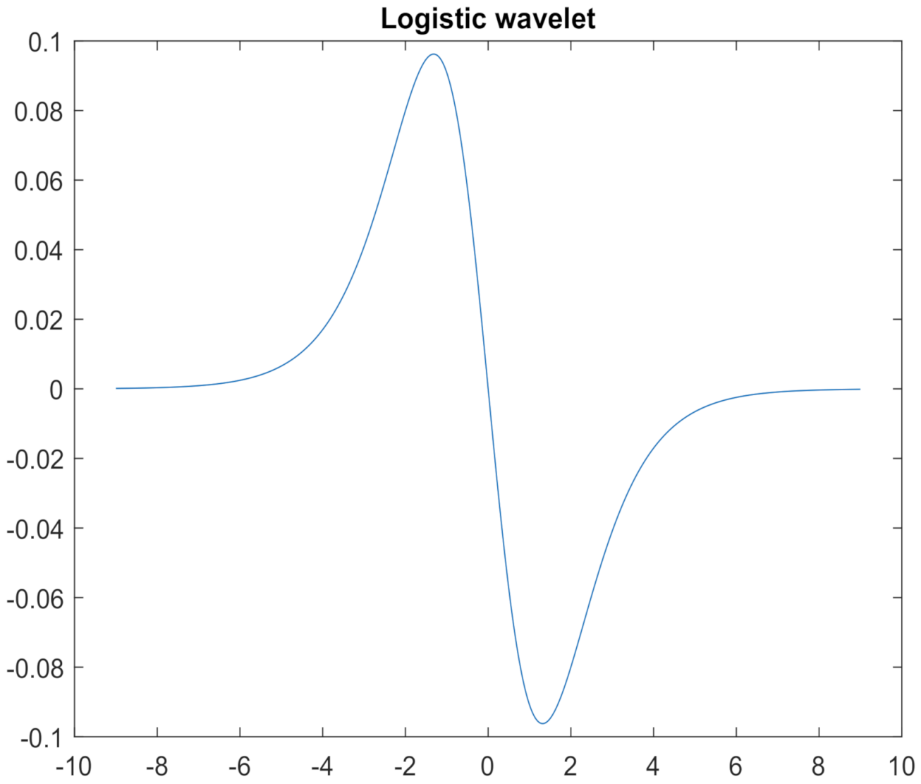
In order to calculate the continuous wavelet transform (CWT) coefficients for $\left({\Delta }^2{y}_n\right)$, we implemented ${\psi }_2\left(x\right)$ into Matlab’s Wavelet Toolbox giving the following definition of the Logistic wavelet:

function [psi,t] = logist(LB,UB,N,∼)

• % LOGISTIC Logistic wavelet.
• % [PSI,T] = LOGIST(LB,UB,N) returns values of
• % the Logistic wavelet on an N point regular
• % grid in the interval [LB,UB].
• % Output arguments are the wavelet function PSI
• % computed on the grid T.
• % This wavelet has [-7 7] as effective support.
• % See also WAVEINFO.
• % Compute values of the Logistic wavelet.
• t = linspace(LB,UB,N); % wavelet support.
• psi = (exp(- 2* t)-exp(-t))./(1+exp(-t)).${}^{\wedge }$3;
• end

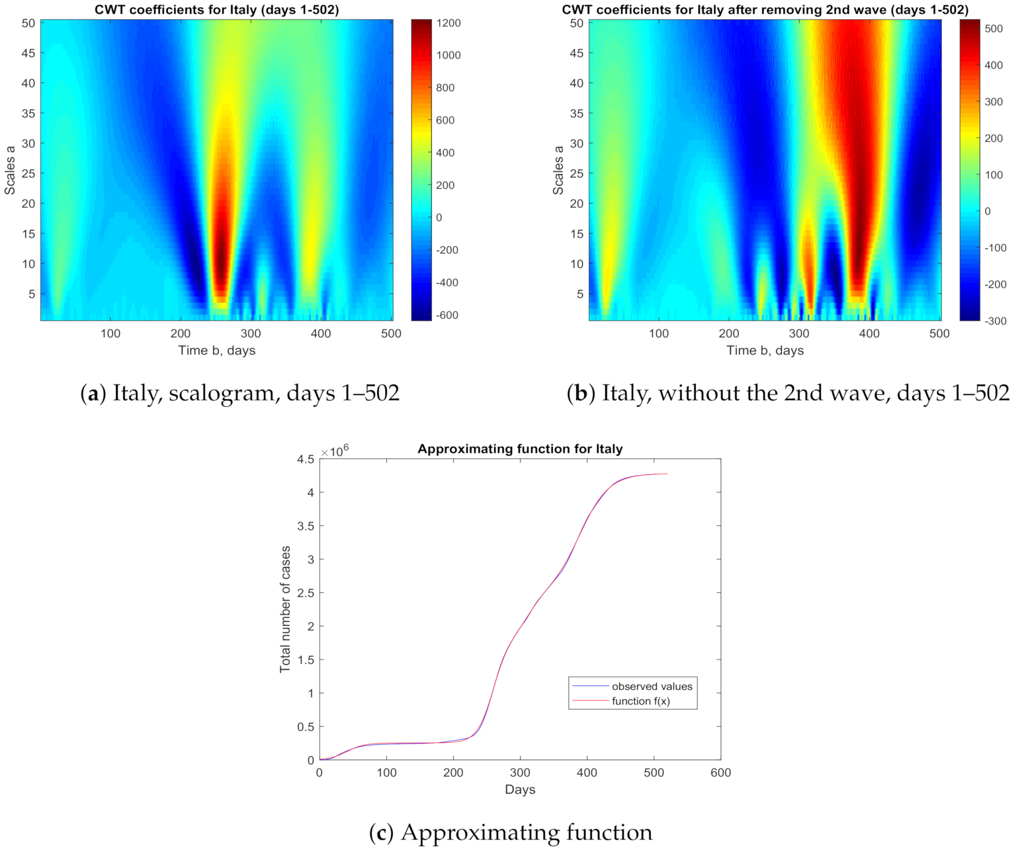
Observations show that successive, relatively large, logistic waves arise at fairly long time intervals. Therefore, usually, the second differences corresponding to all previous waves are small as the next wave unfolds. However, the largest wave (with relatively high values of both the saturation level $u_{max}$ and the parameter a), may be an exception. Therefore, at least for some countries, we perform the next wavelet analysis and calculate the CWT coefficients after subtracting the largest wave. Hence, we calculate the second differences and perform their wavelet analysis for the following new time series

$$z_n=y_n-\frac{u_{i,max}}{1+exp(-\frac{x-b_i}{a_i})},$$

where for $j=i$, the parameters $a_i,b_i,u_{i,max}$ correspond to the largest wave in (20). Moreover, if necessary, we also carry out the wavelet analysis for shorter periods of time.

We find the above mentioned points and parameters either directly by observing the sequence of second differences $\left({\Delta }^2{y}_n\right)$ or read them from the scalograms of the CWT transform of Matlab’s Wavelet Toolbox by using the Logistic wavelet. From the considerations in Section 2.1 and from (9) it follows that parameter b should be determined as that point where the sequence $\left({\Delta }^2{y}_n\right)$ changes sign. Parameter a should be chosen in such a way that the distance between the zero and the maximum of $\left({\Delta }^2{y}_n\right)$ was approximately $1.319a$ (see (9)). Thus, we obtain two parameters defining a logistic function approximating the time series $\left(y_n\right)$. It remains to determine the third parameter of the wave, i.e., its saturation level u. Assuming that $\left(y_n\right)$ follows locally a logistic function ${\displaystyle y_n\approx y\left(n\right)=\frac{u_{max}}{1+exp(-\frac{n-b}{a})}}$ and since by definition it holds

$$y^{″}\left(x\right)=\frac{u_{max}}{a^{3/2}}{\psi }_2^{a,b}\left(x\right),$$

then by (12) we get successively

$$\begin{array}{cc}\hfill {\displaystyle \sum _n}& {\Delta }^2{y}_n{\psi }_2^{a,b}\left(n\right)\approx {\displaystyle \sum _n}{\Delta }^{2}y\left(n\right){\psi }_2^{a,b}\left(n\right)\approx {\int }_{-\infty }^{\infty }{y}^{″}\left(x\right){\psi }_2^{a,b}\left(x\right)dx={\int }_{-\infty }^{\infty }\frac{u_{max}}{a^{3/2}}{\psi }_2^{a,b}\left(x\right){\psi }_2^{a,b}\left(x\right)dx\hfill \\ \hfill & =\frac{u_{max}}{a^{3/2}}{\int }_{-\infty }^{\infty }{\left({\psi }_2^{a,b}\left(x\right)\right)}^{2}dx=\frac{u_{max}}{30a^{3/2}}.\hfill \end{array}$$

(21)

Using (21) we can estimate the saturation level $u_{max}$ as follows

$$u_{max}\approx 30a^{3/2}{\displaystyle \sum _n}{\Delta }^2{y}_n{\psi }_2^{a,b}\left(n\right),$$

(22)

Parameters a and b in (20) can also be estimated by maximizing locally the integral (i.e., the CWT coefficient) on the left-hand side of (21). Hence, we find in the sequence ${\Delta }^2{y}_n$ the best pattern corresponding to the wavelet ${\psi }_2^{a,b}$. The saturation level of a logistic wave can also be estimated as twice the value of the sequence $\left(y_n\right)$ at the point where $\left({\Delta }^2{y}_n\right)$ changes signs (inflection point) or its maximal value multiplied by $1/0.211$ (zero of the third derivative). This approach is especially important for the last wave of the multilogistic function (20), when it is still in its initial or middle stage and has not yet terminated. After this we use the non-linear generalized reduced gradient method, minimizing the RMSE error, to optimize the parameters, mainly saturation levels. All data were collected from the Our World in Data website [27].

We will use the theory to build models for the total cumulative number of individuals reported to be infected by COVID-19 successively in Germany, Italy, Poland, the United Kingdom, the United States, and in the world.

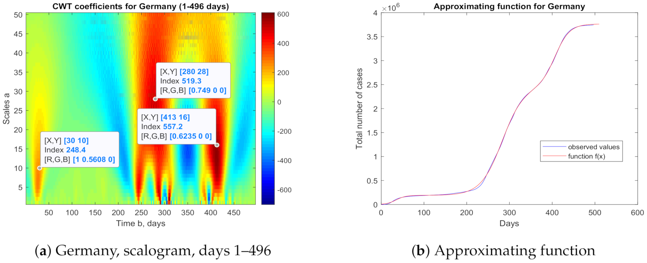
3.1. Germany

Using the example of Germany, we will show in detail the steps leading to the approximating function $f\left(x\right)$ (23). We analyze the data over a period of 496 days from 7 March 2020 ($n=1$) to 15 July 2021 ($n=496$). On the scalogram (Figure 2a) showing CWT coefficients, we can distinguish three large logistic waves. We read for them initially (before optimization) the values of parameters a and b, as well as the value of the CWT coefficient (i.e., the integral (21)). Then, we calculate their estimated saturation levels using Formula (22). We have:

• First wave, $a=10,b=30,\mathrm{CWT}\mathrm{coeff}=248$. Thus, we estimate the saturation level as follows:

  $$u_{max}=248\times 30\times 10\times \sqrt{10}=235,273;$$
• Second wave, $a=28,b=280,\mathrm{CWT}\mathrm{coeff}=519,u_{max}=$ 2,306,883;
• Third wave, $a=16,b=413,\mathrm{CWT}\mathrm{coeff}=557,u_{max}=$ 1,069,440.

Next, we optimize the values of these parameters by minimizing the root mean square error (RMSE) value, which gives:

$$\mathrm{RMSE}=\sqrt{\frac{1}{496}{\displaystyle \sum _{n=1}^{496}}{(y_n-f\left(n\right))}^2}=15,336$$

with the following approximating function

$$f\left(x\right)=\frac{\mathrm{190,654}}{1+exp(-\frac{x-35}{11})}+\frac{\mathrm{2,265,636}}{1+exp(-\frac{x-283}{25})}+\frac{\mathrm{1,308,386}}{1+exp(-\frac{x-407}{17})}.$$

(23)

The approximating function $f\left(x\right)$ (23) is shown in Figure 2b. In the case of Germany, no large, newly emerging logistic wave is visible at that time.

3.2. Italy

In the case of Italy, we analyzed a period of 502 days from 1 March 2020 ($n=1$) to 15 July 2021 ($n=502$) and obtained the following approximating function

$$f\left(x\right)=\frac{\mathrm{253,302}}{1+exp(-\frac{x-41}{13})}+\frac{\mathrm{1,517,214}}{1+exp(-\frac{x-259}{12})}+\frac{\mathrm{693,808}}{1+exp(-\frac{x-311}{15})}+\frac{\mathrm{1,815,925}}{1+exp(-\frac{x-389}{22})},$$

(24)

with the error $\mathrm{RMSE}=$ 12,926. Figure 3 shows scalograms with CWT coefficients and the approximating function (24).

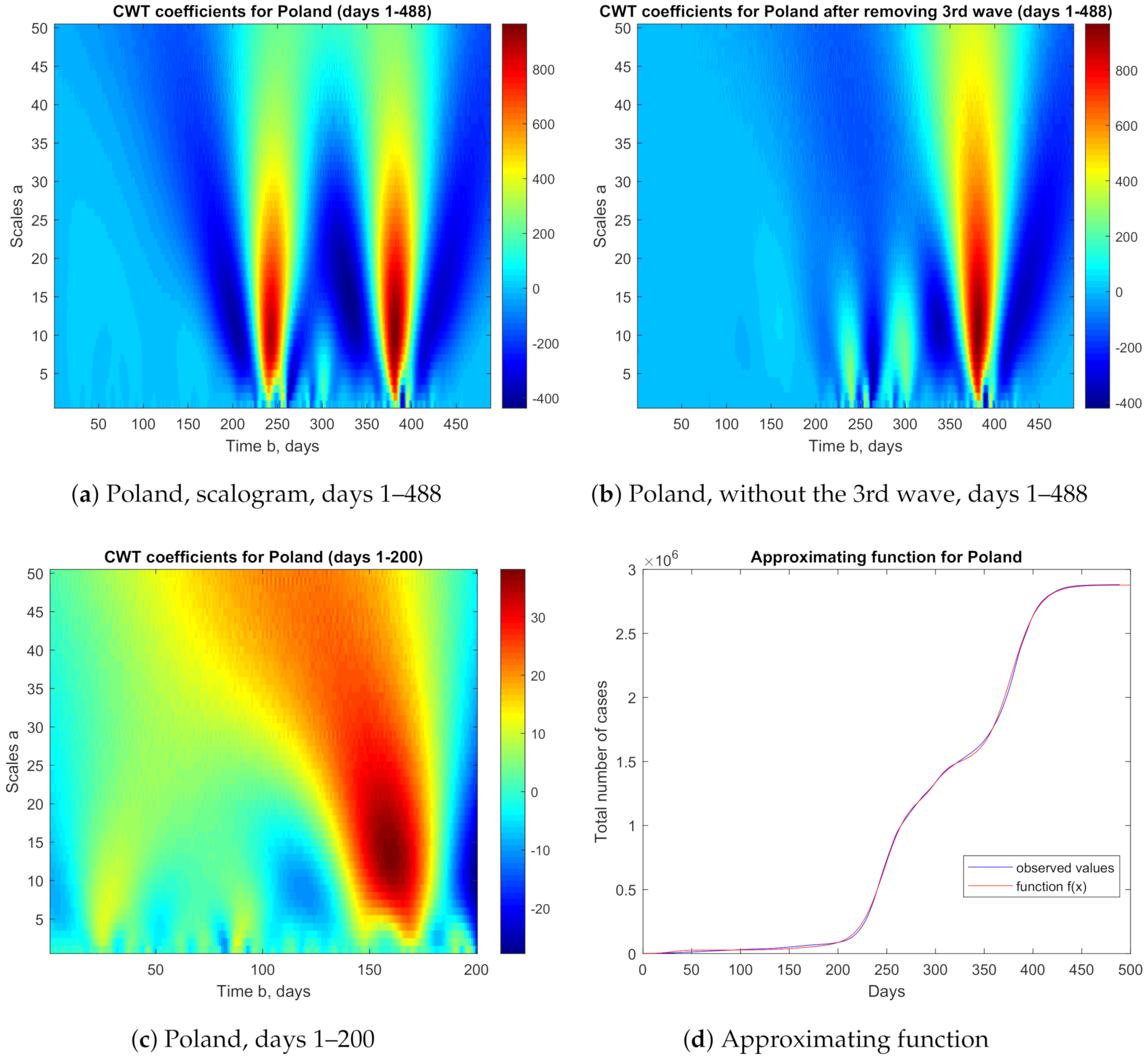
3.3. Poland

We analyzed data over a period of 488 days from 15 March 2020 ($n=1$) to 15 July 2021 ($n=488$). The multilogistic approximating function has the following form

$$\begin{array}{cc}\hfill f\left(x\right)=& \frac{\mathrm{27,659}}{1+exp(-\frac{x-29}{7})}+\frac{\mathrm{30,235}}{1+exp(-\frac{x-160}{15})}+\frac{\mathrm{1,118,196}}{1+exp(-\frac{x-247}{13})}+\frac{\mathrm{237,375}}{1+exp(-\frac{x-301}{7})}\hfill \\ \hfill & +\frac{\mathrm{1,398,841}}{1+exp(-\frac{x-378}{14})},\hfill \end{array}$$

(25)

with the error $\mathrm{RMSE}=$ 13,433. Figure 4 shows scalograms with CWT coefficients and the approximating function (25).

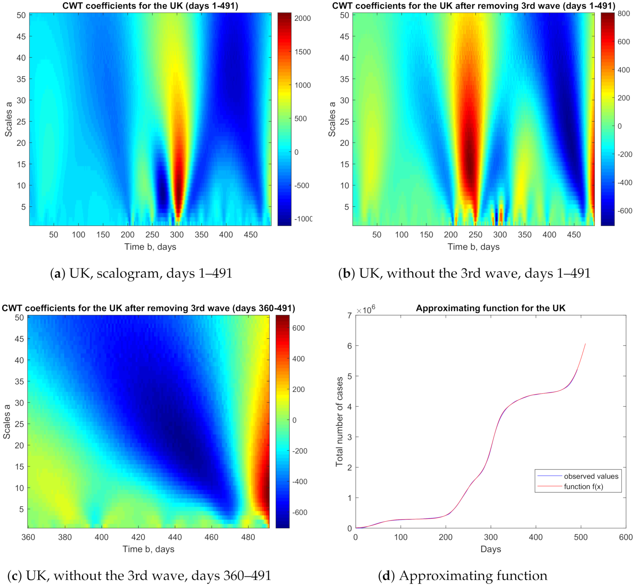
3.4. The United Kingdom

For the UK we analyze the period of 491 days from 12 March 2020 ($n=1$) to 15 July 2021 ($n=491$). Figure 5 shows scalograms with CWT coefficients.

In this case, unlike in previous countries, a new, developing logistic wave is visible on the right in the Figure 5b,c. On July 16 (day 492), this wave has not yet reached its inflection point, as shown by the second differences, which are all positive (

Table 2. A part of the working table for the UK.

Day, n	${\mathit{y}}_{\mathit{n}}$	${\mathbf{\Delta }}^{\mathbf{2}}{\mathit{y}}_{\mathit{n}}$
⋮	⋮	⋮
482	4,896,238	913
483	4,923,476	636
484	4,951,350	1288
485	4,980,512	1054
486	5,010,728	1069
487	5,042,013	1100
488	5,074,398	1125
489	5,107,908	1446
490	5,142,864	2363
491	5,180,183	2295
492	5,219,797

).

With the CWT analysis alone, it would be difficult to determine the parameters of this wave. However, in order to do it we can use the results of Section 2.1. Assuming that the second differences reach their maximum on July 14 (day 490), i.e., it is the zero ($t_1=490$) of the third derivative of the last wave, we can estimate its saturation level. Subtracting from $y_{490}=$ 5,142,864 the saturation levels of all previous four waves, we get about 700,000 cases. Thus, the saturation level of the last wave can be estimated as $u_{max}=$ 700,000/0.211 ≈ 3,300,000. Moreover, assuming that the parameter a is similar to that which was for the other waves, say $a=16$, by (9) we have $b=t_0=t_1+1.319\times 16\approx 511$. After the optimization we get the following approximating function

$$\begin{array}{cc}\hfill f\left(x\right)=& \frac{\mathrm{296,755}}{1+exp(-\frac{x-49}{16})}+\frac{\mathrm{1,492,663}}{1+exp(-\frac{x-238}{16})}+\frac{\mathrm{2,126,051}}{1+exp(-\frac{x-304}{10})}+\frac{\mathrm{519,365}}{1+exp(-\frac{x-355}{18})}\hfill \\ \hfill & +\frac{\mathrm{3,267,991}}{1+exp(-\frac{x-510}{16})},\hfill \end{array}$$

(26)

with the error $\mathrm{RMSE}=$ 12,174. Figure 5 shows also the approximating function (26).

In

Table 3. Forecasting for the UK.

Day, n	Date	${\mathit{y}}_{\mathit{n}}$	$\mathit{f}\left(\mathit{n}\right)$	$|{\mathit{y}}_{\mathit{n}}-\mathit{f}\left(\mathit{n}\right)|$	$|{\mathit{y}}_{\mathit{n}}-\mathit{f}\left(\mathit{n}\right)|/{\mathit{y}}_{\mathit{n}}$
493	2021-07-17	5,262,604	5,273,915	11,311	0.00214
494	2021-07-18	5,307,763	5,313,502	5739	0.00108
495	2021-07-19	5,353,760	5,354,247	487	0.00009
496	2021-07-20	5,401,212	5,396,120	5092	0.00094
497	2021-07-21	5,448,935	5,439,082	9853	0.00180
498	2021-07-22	5,495,427	5,483,091	12,336	0.00224
499	2021-07-23	5,539,655	5,528,095	11,560	0.00208
500	2021-07-24	5,580,660	5,574,038	6622	0.00118
501	2021-07-25	5,618,963	5,620,858	1895	0.00033
502	2021-07-26	5,655,018	5,668,486	13,468	0.00238

(Added in proof), we compare the 10-day forecast with actual data. The last two columns show the forecast error, both absolute and relative. It can be seen that the function $f\left(n\right)$ predicts the trend quite well for a short period. However, it seems more important that the discussed method can be used for early warning of the appearance of new waves. This is in line with Hu et al. [28] comments on the use of wavelet analysis to study the development of infectious diseases.

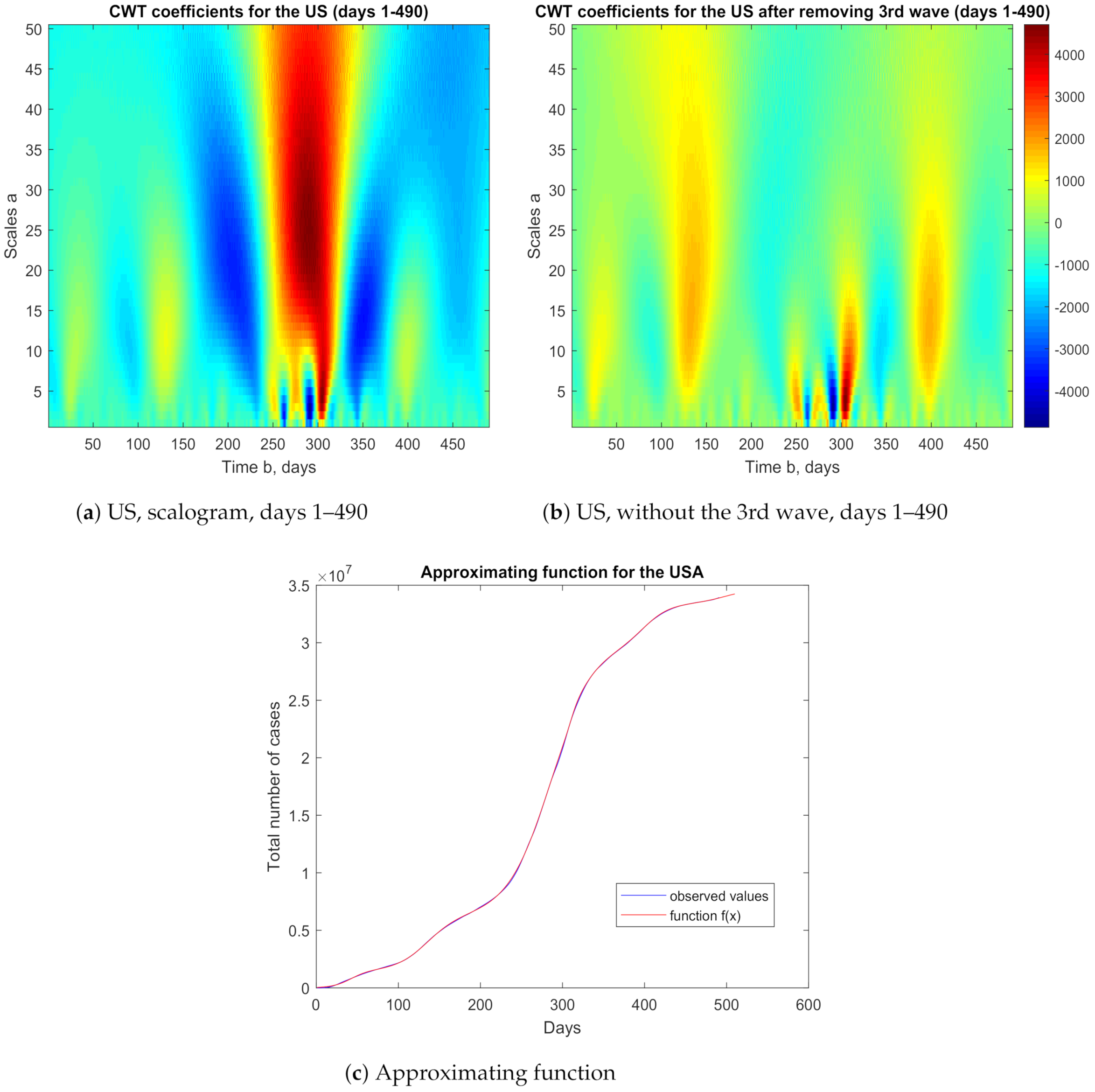
3.5. The United States

In the case of the US, we analyzed the data over a period of 490 days from 13 March 2020 ($n=1$) to 15 July 2021 ($n=490$). The multilogistic approximating function has the following form

$$\begin{array}{cc}\hfill f\left(x\right)=& \frac{\mathrm{1,489,667}}{1+exp(-\frac{x-42}{11})}+\frac{\mathrm{4,777,642}}{1+exp(-\frac{x-135}{19})}+\frac{\mathrm{22,527,836}}{1+exp(-\frac{x-284}{26})}+\frac{\mathrm{996,663}}{1+exp(-\frac{x-311}{4})}\hfill \\ \hfill & +\frac{\mathrm{3,648,578}}{1+exp(-\frac{x-400}{16})}+\frac{\mathrm{1,228,591}}{1+exp(-\frac{x-499}{17})},\hfill \end{array}$$

(27)

with the error $\mathrm{RMSE}=$ 59,106.

The scalograms with CWT coefficients and the approximating function (27) are shown in Figure 6.

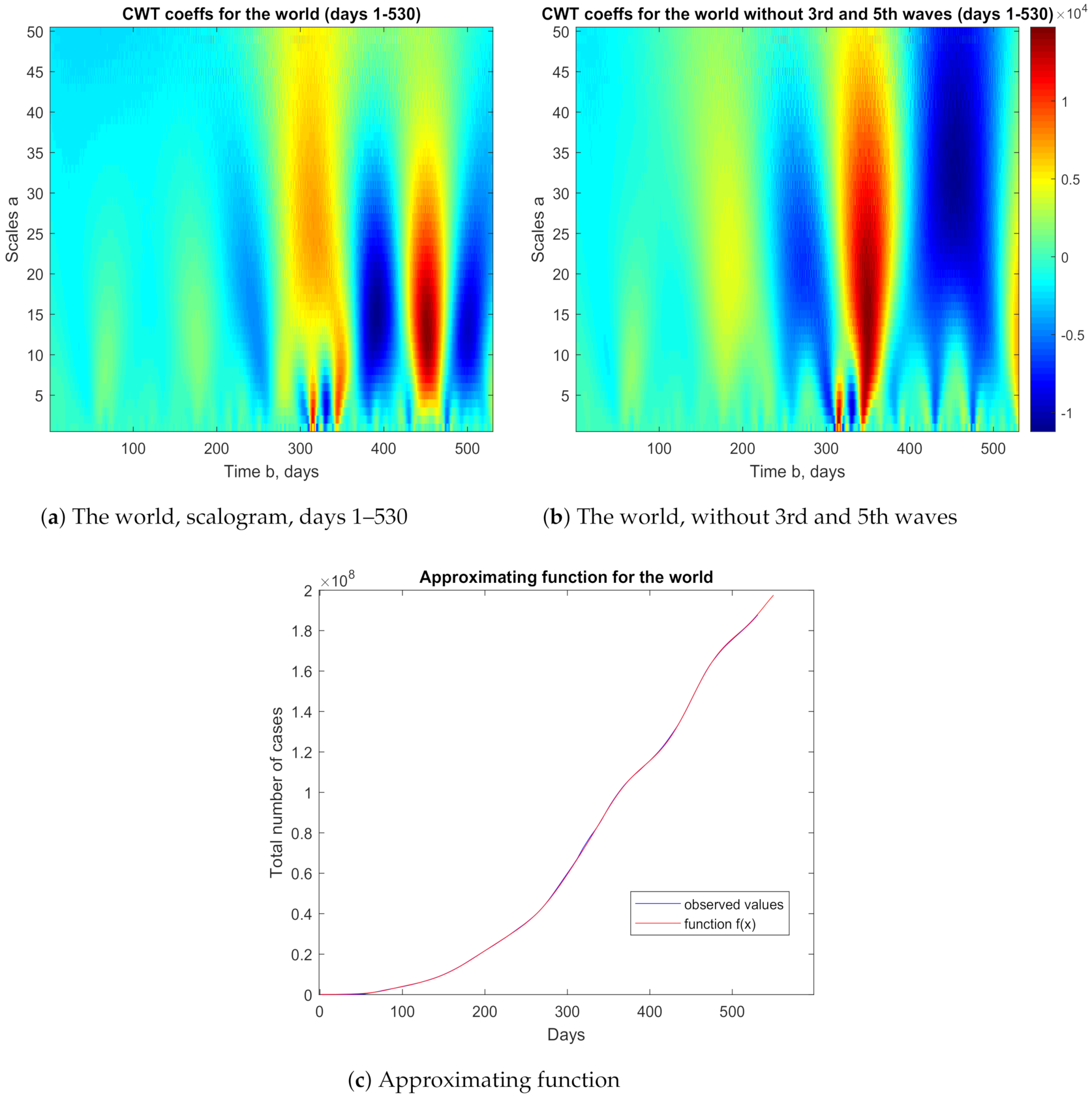
3.6. The World

In the case of the whole world, we analyzed the data over a period of 530 days from 2 February 2020 ($n=1$) to 15 July 2021 ($n=530$). The multilogistic approximating function has the following form

$$\begin{array}{cc}\hfill f\left(x\right)=& \frac{\mathrm{2,951,000}}{1+exp(-\frac{x-83}{12})}+\frac{\mathrm{30,199,966}}{1+exp(-\frac{x-188}{31})}+\frac{\mathrm{42,251,210}}{1+exp(-\frac{x-293}{23})}+\frac{\mathrm{37,503,735}}{1+exp(-\frac{x-348}{19})}\hfill \\ \hfill & +\frac{\mathrm{67,293,529}}{1+exp(-\frac{x-451}{21})}+\frac{\mathrm{27,772,754}}{1+exp(-\frac{x-541}{15})},\hfill \end{array}$$

(28)

with the error $\mathrm{RMSE}=$ 248,525.

The scalograms with CWT coefficients and the approximating function (28) are shown in Figure 7.

4. Discussion

The article deals with the application of the logistic function to the description of phenomena that follow many overlapping sigmoidal trends. We used some properties of the zeros of successive derivatives of the logistic function, in particular their relation to the saturation level.

By using the Eulerian numbers, we defined logistic wavelets of any order and examined their properties, checking for them the general admissibility condition for wavelets. We have added a second order logistic wavelet to the Matlab’s Wavelet Toolbox. Then we performed a wavelet analysis of the time series, whose terms are the second differences of the smoothed total number of individuals infected with the COVID-19 virus in several countries. As a result, we obtained the continuous wavelet transform (CWT) scalograms, from which we could read the distribution of successive logistic waves, and their parameters. Note that the three-dimensional CWT scalograms allow the simultaneous identification of all three parameters of consecutive logistic waves. This has been described in detail using the example of Germany Section 3.1. Other approximation methods do not provide such possibilities. We then optimized the parameters (mainly the saturation levels) minimizing the RMSE error. We have shown in the examples that the multilogistic function, obtained in this way, well approximates the total number of infections. The theory and procedure can be applied to model the total number of infections in any country or a region.

We limited ourselves to identifying the largest logistic waves visible on the scalograms. There are also visible smaller waves, which we have omitted, because they do not contribute much to the explanation of the phenomenon. These could be considered in addition and then the RMSE error would probably be smaller.

The CWT analysis described above makes it possible to estimate the parameters of the logistic waves that have already terminated. In the case of an ongoing, new wave, what we have seen on the example of the UK Section 3.4, we should determine its level of development. In practice, it can be done by determining whether the logistic wave has already reached the inflection point (zero of the second derivative, 50% of the saturation level), which corresponds to a change in the sign in the series of second differences $\left({\Delta }^2{y}_n\right)$. If the inflection point has not yet been reached, we can try to determine whether the wave has reached the previously located zero of the third derivative. This corresponds to a maximum in a series of second differences (this point is about 21% of the saturation level).

It may be considered in a further work, whether the CWT analysis, based on the use of only the positive part of the second-order logistic wavelet, would be helpful in determining the parameters of ongoing waves.

In our further work, we intend to use, in a similar way, the logistic wavelets of higher order (see Section 2.3). Moreover, using appropriate special numbers we are going to define analogous wavelets for the Gompertz function (see some initial calculations [29,30]) or for some generalizations of the logistic function (for preliminary theorems see [31]).