Short-Term Load Forecasting Based on Deep Learning Bidirectional LSTM Neural Network

Abstract

Accurate load forecasting guarantees the stable and economic operation of power systems. With the increasing integration of distributed generations and electrical vehicles, the variability and randomness characteristics of individual loads and the distributed generation has increased the complexity of power loads in power systems. Hence, accurate and robust load forecasting results are becoming increasingly important in modern power systems. The paper presents a multi-layer stacked bidirectional long short-term memory (LSTM)-based short-term load forecasting framework; the method includes neural network architecture, model training, and bootstrapping. In the proposed method, reverse computing is combined with forward computing, and a feedback calculation mechanism is designed to solve the coupling of before and after time-series information of the power load. In order to improve the convergence of the algorithm, deep learning training is introduced to mine the correlation between historical loads, and the multi-layer stacked style of the network is established to manage the power load information. Finally, actual data are applied to test the proposed method, and a comparison of the results of the proposed method with different methods shows that the proposed method can extract dynamic features from the data as well as make accurate predictions, and the availability of the proposed method is verified with real operational data.

1. Introduction

A reliable and accuracy short-term load forecasting system is the basis of energy trade between the customers and electrical utility companies [1,2]. With the increasing penetration of distributed generations and consumer energy systems, the randomness and variability of load profiles bring more challenges for short-term load forecasting systems. Researchers around the world have focused on short-term load forecasting in recent years and tried to get a more accuracy forecasting result using variable new technologies.

The traditional load forecasting method uses statistics [1,3,4], which has appeared in former studies. However, large amounts of precise historical data are needed, which increases the challenges of accurate prediction. Artificial neural network-based methods are the most popular among the data-driven methods due to their strong capability of nonlinear approximation and self-learning. Different types of neural networks such as back propagation (BP) [5], radial basis function (RBF) [6], and extreme learning machines (ELM) [7,8] have been proposed and applied in short-term load forecasting. Furthermore, a regularizing term and the combination of multiple ELM is added to reduce the randomness of traditional ELM in photovoltaic power forecasting in [8]. However, low convergence speed is always an obstacle to the large-scale application of neural networks.

The rapid development of a deep learning framework and artificial intelligence (AI) technology brings more choices for the power system load forecasting. In recent years, convolutional neural network (CNN) [9,10], deep belief network (DBN) [11,12,13], and deep residual networks (DRN) [14] have been developed and applied in load forecasting, which shows a promising prospect in load forecasting areas. These methods can extract the key elements of the load profile. A multiple-input deep convolutional neural network (CNN) model is proposed and applied in the short-term photovoltaic power forecasting in [9], in which solar radiation and ambient temperature combined with the historical output power of a PV system are collected as the input data of the forecasting model. In [10], a deep convolutional neural network-based forecasting method is proposed for the short-term PV power forecasting; here, the original meter data are decomposed into a two-dimensional timescale by convolution kernels and refined into advanced features by a CNN model. Deep belief network is applied in photovoltaic power forecasting in [11]; the proposed methodology is focused on real data capturing to establish the optimum architectural of deep belief network. An improved deep belief network is applied in load forecasting considering demand-side response in [12]; three aspects of the DBN are optimized to dispose the predictive accuracy. The deep belief network method is incorporated into a feed-forward neural network in [13], in which the layer-by-layer unsupervised training procedure is combined with parameters’ fine-tuning based on a supervised back-propagation training method. In [14], a two-stage ensemble strategy of deep residual network is formulated to enhance the generalization capability of load forecasting.

Due to its advantages to solve the vanishing gradient issues, LSTM is more effective than a recurrent neural network to deal with industrial problems that are highly related to time series [15,16,17]. A LSTM neural network has been successfully deployed in many practical applications; it can learn longer-term dependencies due to the associated memory units [18,19,20]. An LSTM architecture-based method is used in a distributed network in [18], in which the LSTM-based structure is used for the linear regression of each node and receives a variable length data sequence with its neighbors to train the LSTM architecture. A video-captioning method based on adversarial learning and LSTM is proposed in [19]; it is used to handle the temporal nature of video data exponential error accumulation. In [20], an attention-based LSTM model with semantic consistency is used to transfer videos to natural sentences. An LSTM neural network is used in multimodal ambulatory sleep detection in [21], and the proposed method can synthesize temporal information accuracy. In [22], nonuniformly sampled variable length sequential data are classified, which is followed by regression by LSTM.

The LSTM neural network also shows significant potential in the prediction field. The authors in [23,24] proposed an LSTM-based framework for the single energy customer load forecasting. In [25], a multi-layer bidirectional RNN based on LSTM and a gated recurrent unit (GRU) is proposed for short-term load forecasting; the proposed method can match different types of load data and is shown to be more accurate. In [26], a forecasting model based on LSTM-DNN is proposed for the photovoltaic power output, available temperature data, and statistical features extracted from the historical photovoltaic output data using stationary wavelet transform. An LSTM neural network is proposed for the prediction of solar irradiance one hour in advance and one day in advance [27,28]; the clearness index was used to classify the type of weather by k-means. A k-means LSTM network model for wind power spot prediction is proposed in [29]; the wind power factors are clustered to generate a new LSTM sub-prediction model.

In [30], the authors proposed five LSTM-based forecasting methods for photovoltaic power prediction, and the prediction capacity is improved by stacking LSTM layers on top of each other. In [31] a one-dimensional convolutional stacked LSTM for load disaggregation is proposed; the deep learning framework is created by stacking several LSTM layers within the hidden layers. The hidden layers are joined reconnections in the LSTM cell. There is no gradient disappearance or gradient explosion problem in the prediction model of the stacked LSTM neural network. However, the long-distance data transmission will cause data loss, which will result in accumulated errors in the process prediction. In order to solve this problem, reverse computing combined with forward computing are introduced to solve the unidirectionality of the memory process in the process of training the data. A feedback mechanism is introduced to improve the front and back association. Combined with the reverse computing, the LSTM neural network has the ability of bidirectional computing, which can overcome the defection of data loss in long-distance transmission. Furthermore, forward and backward propagation prediction make data more dependent and reliable. A multi-layer stacked deep learning style is built for the data training process to improve the information communication between the dataset sequentially.

The main contributions of this paper are as follows: (1) A bidirectional LSTM short-term load forecasting framework model is proposed in this paper, in which reverse computing is combined with forward computing to retrieve the important information hidden in the load profiles and improve the forecasting ability of the time-series problem. (2) A multi-layer stacked bidirectional LSTM prediction structure based on deep learning technology is proposed. The advantages of the multi-layer structure are applied to analyze the load profiles and extract the data essential features. (3) Last, the multi-layer stacked bidirectional LSTM prediction model is approved by using real operational cases, and the evaluation results are compared with other methods.

2. LSTM Neural Network

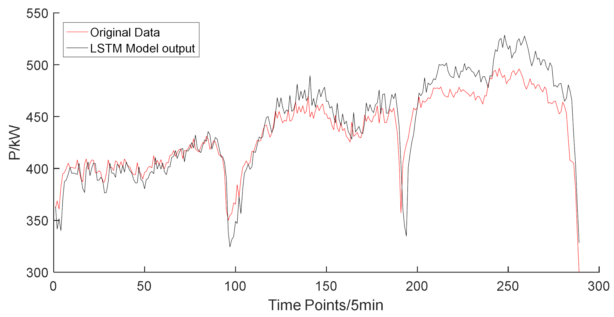
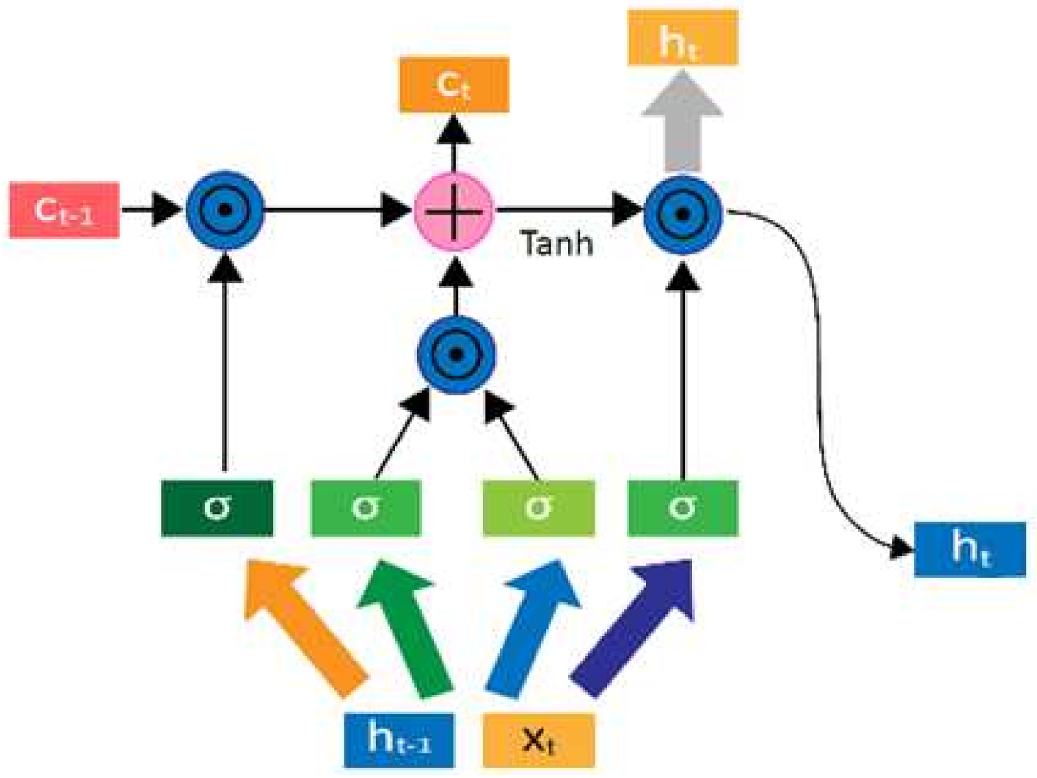
2.1. LSTM Neural Network

The LSTM neural network was proposed in 1997, which is a time-domain deep learning neural network. Compared with traditional recurrent neural network, there are two special parts: the forget gate and the memory unit in the hidden layer of the LSTM neural network. A long-term information stream from the input to output can improve the memory capacity of the neural network in the process of training. The structure of the LSTM cell is shown in Figure 1. It consists of four computing units: namely, the output gate, forget gate, memory unit, and input gate, respectively.

Based on the output $h_{t-1}$ of the last hidden layer and the current input $x_t$, a new value of $f_t$ is generated based on the activation function “Sigmoid”, which determines whether to let the information $C_{t-1}$ learned in the last moment pass through; that is, how much of the last cell state $C_{t-1}$ is saved to the current time $C_t$. The function between $h_{t-1}$,$x_t$ and $f_t$ can be written as:

$$f_t=\sigma \left(W_f\cdot \left[h_{t-1},x_t\right]+b_f\right)$$

(1)

where $\sigma$ is the “Sigmoid” function, and the range of the output value of the “Sigmoid” function is [0,1]. $W_f$ is the weight matrix of the forget gate, $b_f$ is the bias of the forget gate, $f_t$ is the value of the forget gate which decides the forgetting factor of long-term memory information. The value of $f_t$ is between [0,1].

The threshold of LSTM consists of a sigmoid activation function and dot multiplication operation. After the hidden layer of the previous moment enters the forget gate, the function gives the judge information about whether it is updated or not. However, the cell state rolls continuously and runs in the horizontal direction.

$$I_t=\sigma \left(W_t\cdot \left[h_{t-1},x_t\right]+b_i\right)$$

(2)

$${\tilde{C}}_t=\tanh \left(W_{\mathrm{c}}\cdot \left[h_{t-1},x_t\right]+b_c\right)$$

(3)

$$C_t=f_t*C_{t-1}+I_t*{\tilde{C}}_t$$

(4)

where $\tanh$ is the hyperbolic tangent activation function, ${\tilde{C}}_t$ is the temporary unit state of $C_t$, $W_{\mathrm{c}}$ is the weight matrix of the memory unit, $b_c$ is the bias of the memory unit, and $I_t$ is the output value of the input gate. The current cell state $C_t$ is the sum of the original state and the updated state.

$$o_t=\sigma \left(W_o\cdot \left[h_{t-1},x_t\right]+b_o\right)$$

(5)

$$h_t=o_t*\tanh \left(C_{\mathrm{t}}\right)$$

(6)

where $W_o$ is the weight matrix of the output gate, $o_t$ is the output value of the output gate, and $b_o$ is the bias of the output gate. The initial output $h_t$ is obtained through the sigmoid layer, $\tanh \left(C_t\right)$ is between −1 and 1.

The signal passes through the input gate, output gate, and forget gate in turn, and it realizes information storing and maintaining in the current time period. The LSTM structure of the neural network shows that the input variable is transmitted horizontally from input to output directly. Hence, the prediction error will accumulate continuously and suddenly swell in direct proportion with the previous time in the prediction model. Figure 2 shows the LSTM prediction accumulation error in the power load forecasting in one day. The short-term load forecasting method usually takes a day or a week as the training dataset. Three days’ data are taken as sample forecast in Figure 2. The error accumulation occurs in the LSTM prediction results with the increase in the step of the prediction data, and the error will become larger and larger as time goes on.

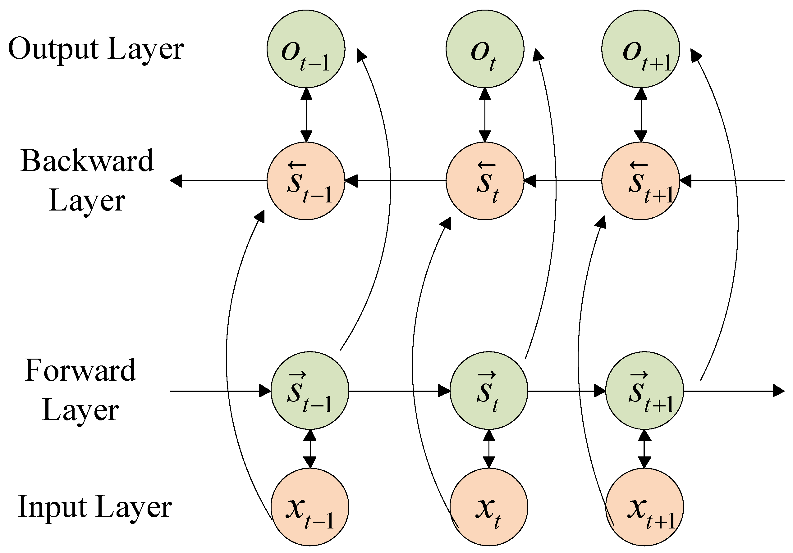
2.2. Bidirectional LSTM Neural Network

In order to overcome the accumulative error problem, a bidirectional LSTM is proposed here, which is shown in Figure 3. The bidirectional LSTM neural network consists of two layers of LSTM structure; one is used to calculate the hidden vector from the front to the back, and the other is used to calculate the hidden vector from the back to the front. The output of the bidirectional LSTM neural network is determined by these two layers.

The bidirectional LSTM neural network is different from the traditional feed-forward mechanism neural network. The internal nodes in each layer do not connect with each other in bidirectional LSTM. A directional loop is introduced in the connection of hidden layers, foregoing information; results are memorized and stored in the memory unit, which can improve the association of single pieces of information in different time series. The current output of the neural network is determined bycombining the previous output and the current input. However, with the increasing amount of input data in the time series, there will be gradient disappearance and gradient explosion problems due to the lack of delay window width.

Based on the traditional LSTM model, the bidirectional LSTM neural network will fully consider the front and back correlation of the load data in time series and improve the model performance for the sequence classification problem especially. During the training process, the input data sequence of the forward layer is the training data, and the backward layer is the reverse copy of the input data sequence. The results of bidirectional structure prediction are determined by the previous input and the latter input, which increases the dependence between the training data to avoid the forgetting of the order information.

Figure 3 shows that the forward layer calculates the forward direction from 1 to $t$, and it saves the output of the forward hidden layer at each moment. The backward layer calculates the reverse time series and saves the output of the backward hidden layer at each moment. Finally, the output of the bidirectional LSTM neural network is calculated by combining the corresponding output results of the forward layer and backward layer at each time point. The bidirectional LSTM neural network can be written as:

$$s_t=f\left(U{x}_t+W{s}_{t-1}\right)$$

(7)

$$s_t^{\prime }=f\left(U^{\prime }{x}_t+W^{\prime }{s}_{t+1}^{\prime }\right)$$

(8)

$${\mathrm{o}}_t=g\left(V{s}_t+V^{\prime }{s}_t\right)$$

(9)

where $s_t$ is the state variable of the hidden layer at time $t$, ${\mathrm{o}}_t$ is the state variable of the output layer at time $t$, $s_t^{\prime }$ is the state variable of the reverse hidden layer at time $t$, $x_t$ is the input vector, $g$ and $f$ are activation functions, $V$, $W$, and $U$ are the weight matrix from the hidden layer to the output layer, the hidden layer, and the input layer to the hidden layer, and $V^{\prime }$, $W^{\prime }$, and $U^{\prime }$ are the corresponding reverse weight matrix. The state weight matrix of the forward layer and the backward layer is not shared information between the two. The forward layer and backward layer are calculated in turn and give the result of each time. The final output ${\mathrm{o}}_t$ depends on the sum of the forward calculation result $s_t$ and the reverse calculation result $s_t^{\prime }$.

3. Multi-Layer Stacked Bidirectional LSTM Neural Network for Short-Term Load Forecasting

The power load profile is affected by the residential electricity behavior, temperature, humidity, etc. It is a multi-dimension nonlinear problem. The bidirectional LSTM neural network solves the accumulated error problem in the training process. Furthermore, the multi-layer bidirectional LSTM neural network is the fusion of a bidirectional neural network based on a deep learning mechanism. A multi-layer forward structure and reverse structure constitute the multi-layer stacked bidirectional LSTM. The multi-layer stacked bidirectional LSTM neural network expands the depth of the bidirectional LSTM neural network. The input data can be learned repeatedly to get an in-depth understanding of the data characteristics and improve the accuracy of load forecasting.

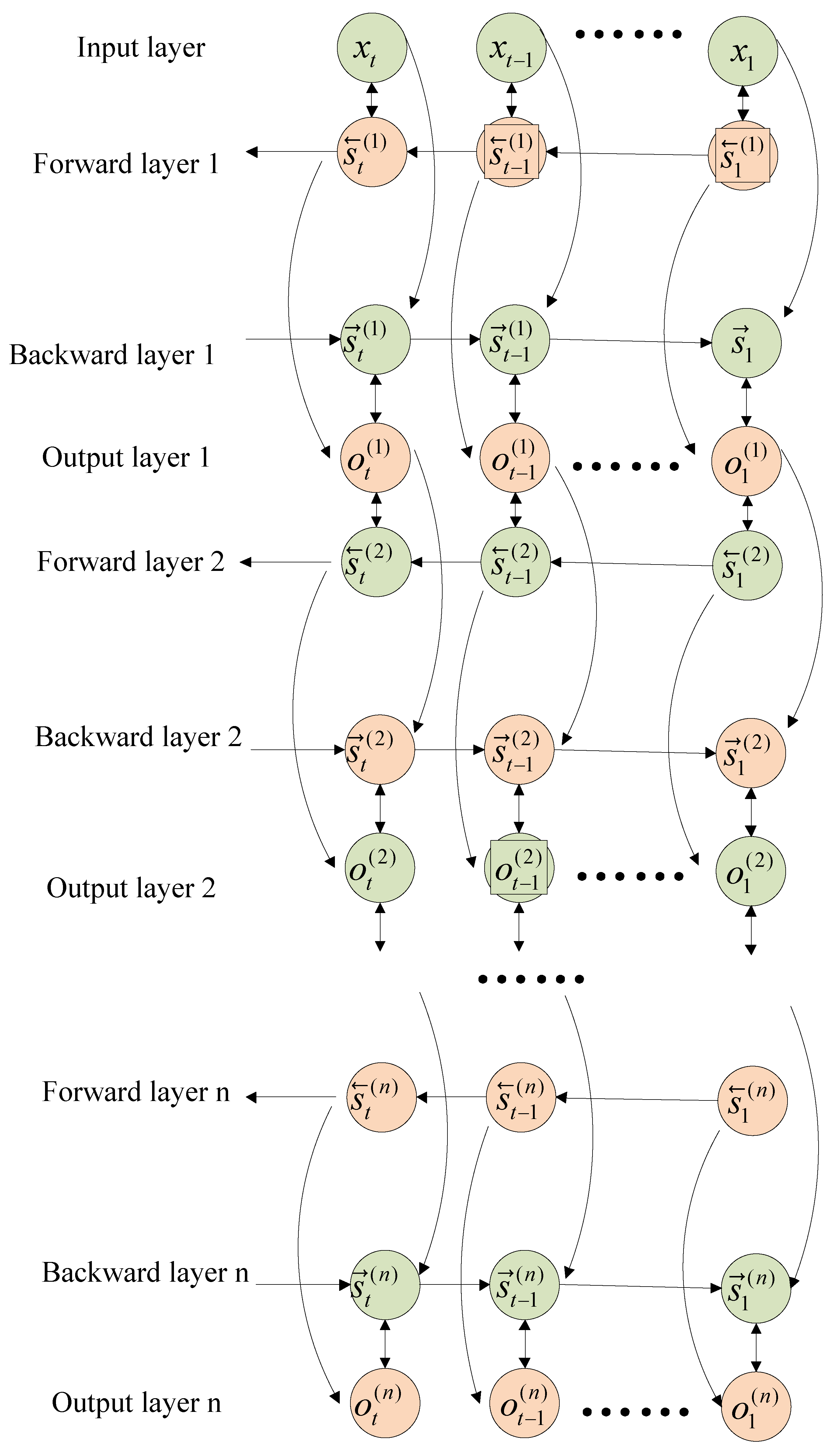
3.1. Multi-Layer Stacked Bidirectional LSTM Neural Network

The system structure of the multi-layer stacked bidirectional LSTM is shown in Figure 4. In the multi-layer stacked structure, every two layers of the LSTM neural network are composed of forward and reverse LSTM networks. The second layer receives the sum of the output results of the first layer of forward and reverse LSTM.

Figure 4 specifies the multi-layer bidirectional LSTM neural network system structure; the output of the multi-layer stacked bidirectional LSTM neural network is determined by the forward and backward results of each layer, and its model can be expressed as follows.

$${\mathrm{o}}_t=g\left(V^{(j)}{s}_t^{(i)}+V^{(i)}{s}_t^{(i)}\right)$$

(10)

$${\mathrm{o}}_t=g\left(V^{(j)}{s}_t^{(i)}+V^{(i)}{s}_t^{(i)}\right)$$

(11)

$$s_t^{(i)}=f(U^{*(i)}{{s_t}^{\prime }}^{(-1)}+W^{(i)}{s}_{t+1}^{\prime })$$

(12)

$$s_t^{(1)}=f\left(U^{(1)}{x}_t+W^{(1)}{s}_{t-1}\right)$$

(13)

$${{s_t}^{\prime }}^{(1)}=f\left({U^{\prime }}^{(1)}{x}_t+{W^{\prime }}^{(1)}{s}_{t-1}^{\prime }\right)$$

(14)

where $s_t^i$ and $s_{t-1}^i$ are the state variables of the $i^{th}$ hidden layer at $t-1$ and $t$ time, respectively. The forward and reverse calculations do not share the weight information. $V^{(i)}$, $U^{(i)}$, and $W^{(i)}$ are the weight matrix between the input layer, hidden layer, and output layer. In the reverse calculation, $V^{\prime }(i)$, $U^{\prime }(i)$, and $W^{\prime }(i)$ are the corresponding inverse weight matrix, respectively. $i$ is the number of bidirectional LSTM layers, and $i=0,1,2\cdots \infty$ represents the value of the output layer.

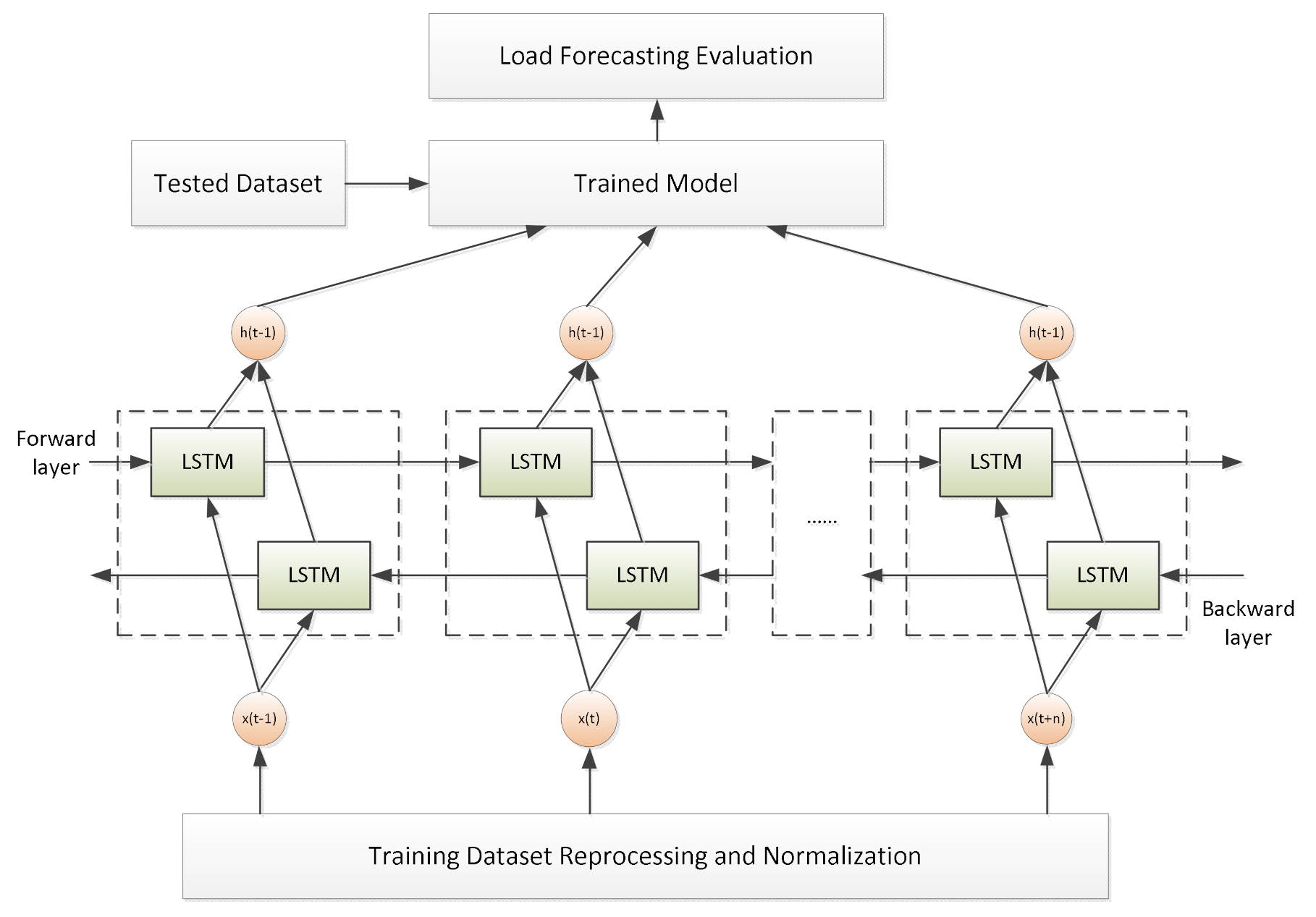
3.2. Multi-Layer Stacked Bidirectional LSTM Based Load Forecasting

The essential concept of the proposed improved LSTM neural network consists of obtaining the statistical analysis of the power load by reconstructing the training sample data. The multi-layer stacked bidirectional LSTM network is trained to perform the forecast of the power load for the next 24 h. The prediction process of the proposed model can be divided into the follow steps and shown in Figure 5.

Step 1: Data preparation. Historical data of the power load profiles are collected and pre-processed to remove any outlier or incorrect data before the training process. However, the original data are not standard enough to use directly. Normalization is a common method to normalize original data structures in system modeling, and the original data become dimensionless after normalization, which can increase the convergence speed of the neural network. After normalization, the value of the original data is between the range of [0,1]. There are many normalization methods such as min–max scaling, Z-score standardization method, and decimal scaling. In this paper, a linear normalization method based on min–max scaling is used, which can be written as follows:

$$x^{*}=\frac{x-x_{min}}{x_{max}-x_{min}}.$$

(15)

$x_{max}$ and $x_{min}$ are the maximum and minimum values of the sample data of power load, $x$ is the original value of the sample data, and $x^{*}$ is the normalized value of the original data.

Step 2: Network training. The forward value of input at t = 1 and the reverse state value of input at t = T (T is the last sampling time of the training dataset) are unknown, which are generally set to a fixed value (0.5) in the training process. Additionally, the derivative of the forward value of input at T = t and the original value of the reverse state of t = 1 are generally set to zero. It is assumed that the later information is not very important for the current information updated. The process of network training contains the following:

(1) Forward transfer. With the time sequence of 1 < t <= T, training data are input from the cell of the bidirectional LSTM, and the predicted outputs are determined. Forward passes are only for forward states (from t = 1 to t = T) and backward states (from t = T to t = 1). The output cells were transferred forward, and the n-th layer forward predicted output is calculated.

(2) Backward transfer: The derivative of the partial objective function is calculated for the forward transfer time period with 1 < t <= T. The backward LSTM cells are calculated based on the forward value of 1 < t <= T and the reverse value of 1 < t <= T. The reversed prediction output is calculated.

(3) Weight matrix updating. Based on the loss function of the neural network during the training process, the weight matrix is calculated and updated.

(4) Result output. Based on the bidirectional calculation, the parameters of the prediction model of LSTM neural network are estimated.

3.3. Evaluation Index

In this paper, the mean absolute error (MAE), root mean square error (RMSE), and mean absolute percentage error (MAPE) are used to evaluate the error of prediction results. MAPE, RMSE, and MAE are common indicators to evaluate the accuracy of the proposed model based on the measurement value and estimated value. The definition of the indicators is shown in Equations (16)–(18). MAE is the estimated indictor, which is used as the measurement value. RMSE is used to evaluate the deviation between the observed value and the true value; it is sensitive to outliers. MAPE is used to evaluate the relative errors between the average observed value and the true value on the test. MAE can reflect the error distribution during the time series, while MAPE normalizes the error at different points and reduces the effect of the absolute errors of the outliers.

$$MAPE=\frac{1}{n}{\displaystyle \sum _{i=1}^n\frac{\left|x_i-{\widehat{x}}_i\right|}{x_i}}\times 100\%$$

(16)

$$RMSE=\sqrt{\frac{1}{n}{\displaystyle \sum _{i=1}^n{\left|x_i-{\widehat{x}}_i\right|}^2}}$$

(17)

$$MAE=\frac{1}{n}{\displaystyle \sum _{i=1}^n\left|x_i-{\widehat{x}}_i\right|}$$

(18)

$n$ is the number of sample data, $x_i$ is the real value, and ${\widehat{x}}_i$ is the predicted value.

4. Simulation and Experimental Analysis

In this section, we evaluate the performance of the proposed multi-layer stacked bidirectional LSTM neural network for short-term load forecasting, and the key parameters of the model are discussed as well. Moreover, the comparison between the proposed method and previous work are also assessed. All models were executed in a computer with a CPU clock speed of 3.0 GHz and 8 GB of RAM. The hidden layer of the proposed model is 100, the hidden node is 8, the initial value of training learning rate is 0.01, and the number of model training iterations is 100.

4.1. Dataset for Load Forecasting

The databases used in the paper were obtained from the station in the southwest of China with an AC power voltage of 35 kV. The dataset contains a 3-year power load profile with the sampling time of 15 min. The dataset is a mixed dataset that contains different types of loads such as resident load, commercial load, and industrial load. The dataset was pre-processed in order to separate the relevant data and select the predictive features in the models. Here, we separated the dataset into different types for the load forecasting based on days and season characteristics. The pre-processing of the dataset is shown in Section 3.2, and the forecasting models were trained and tested using a 1-year sample dataset where the first 80% is used for model training and the remaining 20% is used to test the performance of the proposed model.

4.2. Neural Network Structure Determine

Prediction accuracy has a significant relationship with the depth of the bidirectional LSTM neural network. The dynamic characteristics of the load data will be extracted based on the interaction of the different layers of the neural network. The internal relevance information of the load profiles will be deep learned with the different stacked layers, and the nonlinearity of the load sequence can be described in different dimensions. The parameters of the input units, forget units, and output units of the proposed model are shown in

Table 1. The parameters of the equivalent model.

Input Gate	0.023	0.020	0.120	0.127	0.033	0.975	0.044	0.037	0.579	0.035
	0.044	0.049	0.017	0.012	0.034	0.025	0.041	0.001	0.043	0.037
	0.027	0.025	0.135	0.128	0.070	0.975	0.049	0.043	0.540	0.007
	0.025	0.047	0.042	0.029	0.034	0.025	0.048	0.043	0.005	0.040
Forget Gate	0.024	0.006	0.030	0.008	0.032	0.015	0.050	0.016	0.024	0.005
	0.012	0.015	0.013	0.046	0.013	0.045	0.041	0.048	0.050	0.019
	0.049	0.044	0.046	0.005	0.000	0.023	0.015	0.046	0.019	0.037
	0.007	0.014	0.030	0.007	0.043	0.016	0.044	0.025	0.047	0.037
Output Gate	0.030	0.002	0.043	0.038	0.005	−0.033	0.049	0.001	0.012	0.014
	0.006	0.024	0.012	0.001	0.046	0.043	0.049	0.036	0.039	0.014
	0.008	0.048	0.029	0.037	0.038	−0.044	0.023	0.012	0.002	0.035
	0.021	0.045	0.002	0.017	0.006	0.048	0.019	0.020	0.023	0.012

.

The prediction accuracy of the different layers of the LSTM neural work is shown in Figure 6. It can be seen that the proposed multi-layer bidirectional LSTM neural network is an effective method and is accurate enough for the load forecast problem. Furthermore, with the increasing numbers of layers, the prediction result will be more accurate. However, when there are four layers, the prediction accuracy will increase, on the contrary. It is said that three layers is suitable for the prediction of the load sequence data in this paper.

Table 2. Error of different stacked layers of bidirectional LSTM.

Bi-LSTM Layers	1	2	3	4	5
MAPE (%)	0.51	0.465	0.405	0.41	0.41

shows the prediction errors of MAPE between the different layers of the different neural network model.

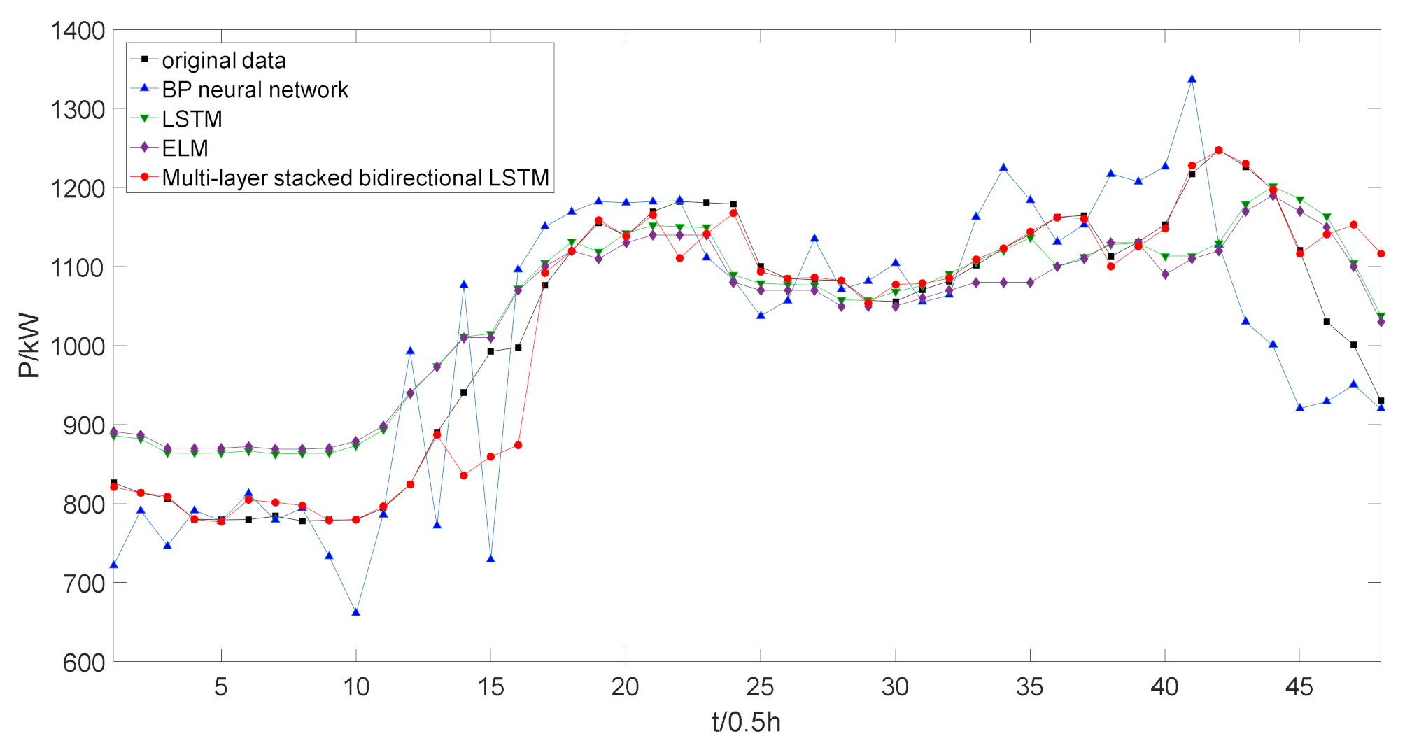
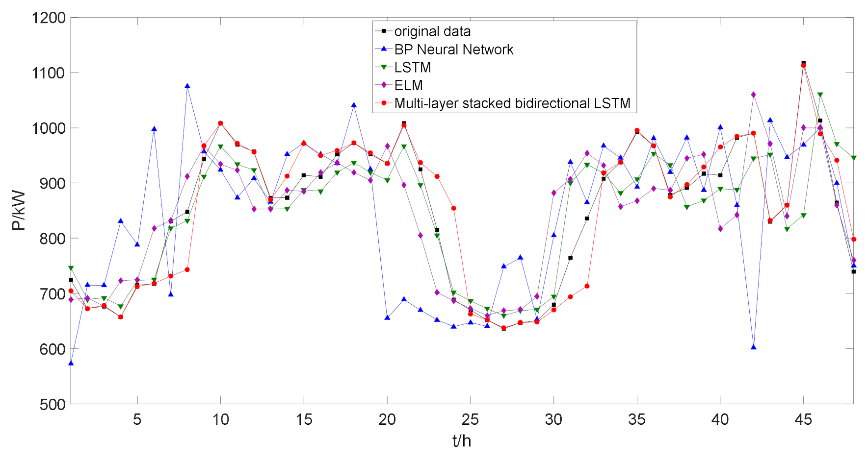
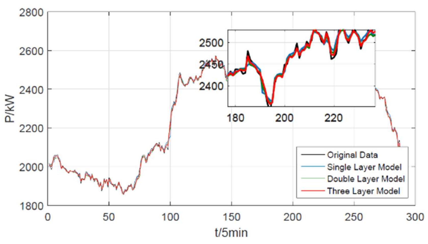
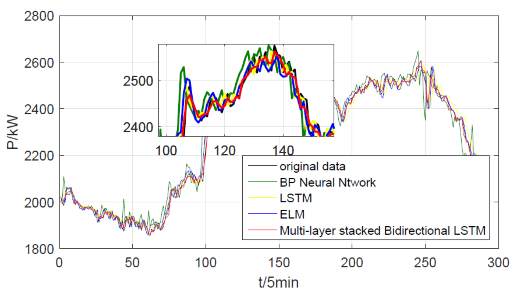
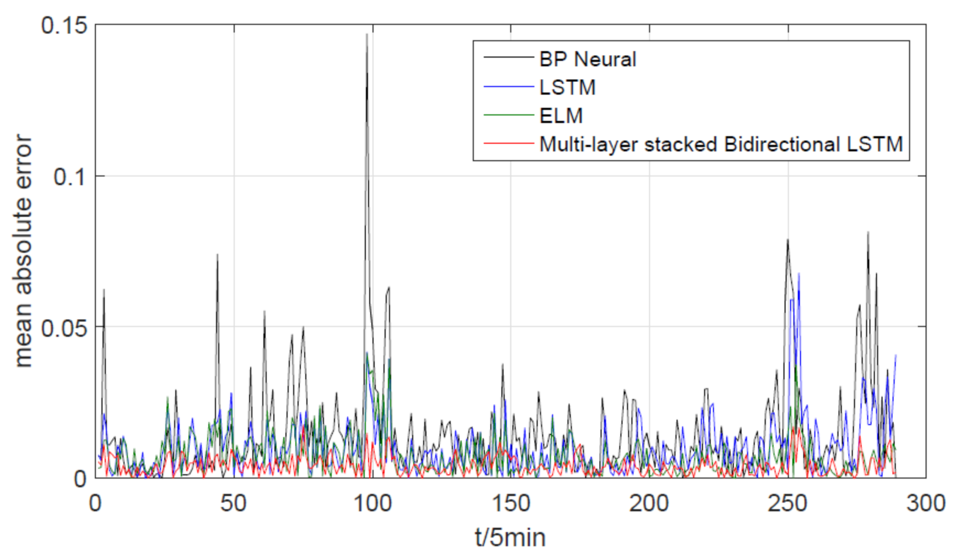
4.3. Method Comparison

In order to show the high performance of the multi-layer stacked bidirectional LSTM neural network in short-term load forecasting, different methods that contain a BP neural network, ELM, traditional LSTM, and multi-layer stacked bidirectional LSTM model are discussed in this paper. The prediction results all the methods tested in this paper followed the same trend with the real load power shown in Figure 7. It can be seen that the multi-layer stacked bidirectional LSTM neural network will be more competitive, and the error comparison of those methods is shown in

Table 3. Error comparison of different prediction models.

Prediction Model	BP	LSTM	ELM	Proposed Method
MAPE (%)	1.485	1.03	0.77	0.405
RMSE	2.95	1.921	1.369	0.706
MAE	33.564	23.236	17.07	9.341

, where the MAPE, RMSE, and MAE index are calculated and compared for one day over 24 h. From Table 3, the average MAPE of the proposed method prediction model is 0.4137%; however, the average MAPE values of the BP, LSTM, and ELM models are 1.485%, 1.030%, and 0.77%, respectively. The average RMSE of the proposed method prediction model is 0.706, and those of the BP, LSTM, and ELM models are 2.95, 1.921, and 1.369, respectively.

Different time interval errors are calculated between ELM, LSTM, BP, and the proposed method in

Table 4. Error comparison of different prediction models in a two-hour interval.

Forecast Time Interval	BP [6]			LSTM [21]			ELM [8]			Proposed Method
	MAPE%	RMSE	MAE	MAPE%	RMSE	MAE	MAPE%	RMSE	MAE	MAPE%	RMSE	MAE
0–2 h	0.73	28.53	14.76	0.59	15.94	11.79	0.58	14.21	11.58	0.35	9.36	7.13
2–4 h	0.92	33.16	17.71	1.18	26.11	22.66	1.11	25.33	21.56	0.49	10.8	9.39
4–6 h	1.62	40.76	30.47	1.01	23.14	19.18	1.08	23.17	20.49	0.41	9.09	7.7
6–8 h	1.71	40.38	35.08	1.03	25.62	21.21	0.92	23.4	18.96	0.52	12.96	10.66
8–10 h	2.67	90.05	60.54	1.22	38.12	28.11	1.26	41.67	28.95	0.49	14.95	11.43
10–12 h	1.1	30.61	27.58	0.79	24.86	19.93	0.65	21.26	16.38	0.39	11.89	9.96
12–14 h	1.27	36.6	30.36	0.66	22.32	15.65	0.57	18.78	13.51	0.43	12.9	10.41
14–16 h	1.05	32.59	25.15	0.56	18.35	13.4	0.61	17.76	14.67	0.39	11.73	9.51
16–18 h	0.95	28.58	23.3	0.78	23.36	19.12	0.43	13.44	10.37	0.27	7.96	6.54
18–20 h	1.09	33.3	27.2	1.0	30.51	25.11	0.56	17.02	14.01	0.32	9.82	8.03
20–22 h	2.27	78.7	57.12	1.85	65.6	46.68	0.93	31.81	23.52	0.48	16.9	11.99
22–24 h	2.42	73.32	54.88	1.57	41.71	35.33	0.48	13.01	10.8	0.42	12.76	9.56

. The two-hour interval forecasting results fluctuate in different evaluation indexes. However, the total evaluation indexes of the proposed method are at the minimum in one day, and the quantitate analysis forecasting errors are calculated and shown in Figure 8. Here, it can be seen that proposed method based on the multi-layer bidirectional LSTM prediction model better grasps the prediction sample information and has a more competitive forecasting performance. The multi-layer stacked bidirectional LSTM neural network model can retain the original characteristics of the load sequences and reduce the data error by incorporating errors in unsupervised training, which can enhance the robustness of the predictive model.

Different samples of training data will significantly affect the robustness of the load forecasting model. The load will be more accurate with a smaller sample in the training dataset. With 48 or 24 measurement points, the training dataset will be more random, which will increase the difficulty of the load prediction. In this paper, a sample dataset with 48 measurement points is used for the training of the proposed method to verify the robustness of the proposed method and compare it with other methods. Figure 9 shows the comparison of the load forecasting results with a half-hour training dataset; the proposed method is accurate enough to track the load profiles based on deep learning, which can extract the internal characteristics of the discrete sample load data and improve the robustness of the proposed method with the multi-layer bidirectional training mechanism. The MAPE of the proposed method is 2.39%, as shown in

Table 5. The error between different methods.

Prediction Model	BP	LSTM	ELM	Proposed Method
MAPE (%)	6.77	5.44	5.61	2.39
RMSE	91.9627	64.244	67.237	50.827
MAE	69.535	51.158	56.03	23.763

.

Furthermore, in order to verify the generalization ability of the proposed method for the more complex environments on special days such as the weekend or a holiday, study cases are tested with the historical day based on different measurement points; these are shown in Figure 10 and Figure 11. It can be seen that the prediction results of the load profile can track the measurement data accuracy in different sample time intervals, and the sampling time will influence the prediction results. The results in Figure 10 and Figure 11 show that the proposed multi-layer stacked bidirectional LSTM method is more accurate than the other methods mentioned such as the BP neural network, ELM, and traditional LSTM neural network.

5. Conclusions

Accurate short-term load forecasting is a huge challenge due to the complexity of the electrical load composition in modern power systems. In this paper, based on the traditional LSTM neural network, a multi-layer stacked type short-term load forecasting method is proposed. Reverse computing combined with forward computing is designed to solve the unidirectionality of the memory process during the training period. The output gate can collaborate the implied information in the historical load series. Furthermore, a multi-layer stacked deep learning style for the neural network is proposed to perceive a low-level features form of power load and form a more abstract high-level representation of load characteristics. At last, a load forecasting frame based on the multi-layer bidirectional LSTM neural network is proposed that contains neural network model construction, historical load profile training, and load forecasting. In the experiments, the real operational load data of a substation are tested, and the performance of the proposed method is tested and evaluated. The results show that the proposed multi-layer stacked bidirectional LSTM neural network method has high performance and is more accurate than the others. The proposed method can retain the original information as much as possible and has a strong memory function to extract the relevant information from historical load sequences.

However, with the increase in the sequence length of the problem, the efficiency of the proposed method will reduce because the capacity of the memory units is limited. There are four fully connected layers in each cell in the LSTM neural network; it needs a lot of computing time in a deep stacked LSTM neural network. Future works will focus on the industrial application of the proposed method with a more complex dataset. (1) We built an online load forecasting system. The application of load forecasting is employed for the dispatch of the power system, which is working all the time. Hence, an online and rolling load forecasting system using the historical load data is the basis of this work. (2) We corrected the load forecasting results. If the load forecast results deviate greatly, the forecast points are corrected based on the data before and after time points.

References

1. Quilumba, F.L.; Lee, W.J.; Huang, H.; Wang, D.Y.; Szabados, R.L. Using smart meter data to improve the accuracy of intraday load forecasting considering customer behavior similarities. IEEE Trans. Smart Grid 2014, 6, 911–918. [Google Scholar] [CrossRef]
2. Xu, D.; Wu, Q.; Zhou, B.; Li, C.; Bai, L.; Huang, S. Distributed multi-energy operation of coupled electricity, heating and natural gas networks. IEEE Trans. Sustain. Energy 2019, 11, 2457–2469. [Google Scholar] [CrossRef]
3. Al-Hamadi, H.M.; Soliman, S.A. Short-term electric load forecasting based on Kalman filtering algorithm with moving window weather and load model. Electr. Power Syst. Res. 2004, 68, 47–59. [Google Scholar] [CrossRef]
4. Ceperic, E.; Ceperic, V.; Baric, A. A strategy for short-term load forecasting by support vector regression machines. IEEE Trans. Power Syst. 2013, 28, 4356–4364. [Google Scholar] [CrossRef]
5. Kaur, A.; Nonnenmacher, L.; Coimbra, C.F. Net load forecasting for high renewable energy penetration grids. Energy 2016, 114, 1073–1084. [Google Scholar] [CrossRef]
6. Cecati, C.; Kolbusz, J.; Rozycki, P.; Siano, P.; Wilamowski, B.M. A novel RBF training algorithm for short-term electric load forecasting and comparative studies. IEEE Trans. Ind. Electron. 2015, 62, 6519–6529. [Google Scholar] [CrossRef]
7. Teo, T.T.; Logenthiran, T.; Woo, W.L. Forecasting of photovoltaic power using extreme learning machine. In Proceedings of the IEEE Innovative in Smart Grid Technologies-Asia (ISGT ASIA), Bangkok, Thailand, 3–6 November 2015; pp. 1–6. [Google Scholar]
8. Teo, T.T.; Logenthiran, T.; Woo, W.L.; Abidi, K. Forecasting of photovoltaic power using regularized ensemble extreme learning machine. In Proceedings of the IEEE Region 10 Conference (TENCON), Singapore, 22–25 November 2016; pp. 455–458. [Google Scholar]
9. Huang, C.J.; Kuo, P.H. Multiple-input deep convolutional neural network model for short-term photovoltaic power forecasting. IEEE Access 2019, 7, 74822–74834. [Google Scholar] [CrossRef]
10. Zang, H.; Cheng, L.; Ding, T.; Cheung, K.W.; Liang, Z.; Wei, Z.; Sun, G. Hybrid method for short-term photovoltaic power forecasting based on deep convolutional neural network. IET Gener. Transm. Distrib. 2018, 12, 4557–4567. [Google Scholar] [CrossRef]
11. Neo, Y.Q.; Teo, T.T.; Woo, W.L.; Logenthiran, T.; Sharma, A. Forecasting of photovoltaic power using deep belief network. In Proceedings of the 2017 IEEE Region 10 Conference (TENCON), Penang, Malaysia, 5–8 November 2017. [Google Scholar]
12. Kong, X.; Li, C.; Zheng, F.; Wang, C. Improved deep belief network for short-term load forecasting considering demand-side management. IEEE Trans. Power Syst. 2019, 35, 1531–1538. [Google Scholar] [CrossRef]
13. Dedinec, A.; Filiposka, S.; Kocarev, L. Deep belief network based electricity load forecasting: An analysis of Macedonian case. Energy 2016, 115, 1688–1700. [Google Scholar] [CrossRef]
14. Chen, K.J.; Chen, K.L.; Wang, Q.; He, Z.; Hu, J.; He, J. Short-term load forecasting with deep residual network. IEEE Trans. Smart Grid 2018, 10, 3943–3953. [Google Scholar] [CrossRef] [Green Version]
15. Ergen, T.; Kozat, S.S. Efficient online learning algorithms based on LSTM neural networks. IEEE Trans. Neural Netw. Learn. Syst. 2017, 29, 3772–3783. [Google Scholar] [PubMed] [Green Version]
16. Greff, K.; Srivastava, R.K.; Koutník, J.; Steunebrink, B.R.; Schmidhuber, J. LSTM: A search space odyssey. IEEE Trans. Neural Netw. Learn. Syst. 2016, 28, 2222–2232. [Google Scholar] [CrossRef] [Green Version]
17. Feng, Y.; Zhang, T.; Sah, A.P.; Han, L.; Zhang, Z. Using appearance to predict pedestrian trajectories through disparity-guided attention and convolutional LSTM. IEEE Trans. Veh. Technol. 2021, 70, 7480–7494. [Google Scholar] [CrossRef]
18. Ergen, T.; Kozat, S.S. Online training of LSTM networks in distributed systems for variable length data sequences. IEEE Trans. Neural Netw. Learn. Syst. 2017, 29, 5159–5165. [Google Scholar] [CrossRef] [Green Version]
19. Yang, Y.; Zhou, J.; Ai, J.; Bin, Y.; Hanjalic, A.; Shen, H.T.; Ji, Y. Video captioning by adversarial LSTM. IEEE Trans. Image Process. 2018, 27, 5600–5612. [Google Scholar] [CrossRef] [Green Version]
20. Gao, L.; Guo, Z.; Zhang, H.; Xu, X.; Shen, H.T. Video captioning with attention-based LSTM and semantic consistency. IEEE Trans. Multimedia 2017, 19, 2045–2055. [Google Scholar] [CrossRef]
21. Sano, A.; Chen, W.; Martinez, D.L.; Taylor, S.; Picard, R.W. Multimodal ambulatory sleep detection using LSTM recurrent neural networks. IEEE J. Biomed. Health Inform. 2018, 23, 1607–1617. [Google Scholar] [CrossRef]
22. Sahin, S.O.; Kozat, S.S. Nonuniformly sampled data processing using LSTM networks. IEEE Trans. Neural Netw. Learn. Syst. 2018, 30, 1452–1462. [Google Scholar] [CrossRef]
23. Mohan, N.; Soman, K.; Kumar, S.S. A data-driven strategy for short-term electric load forecasting using dynamic mode decomposition model. Appl. Energy 2018, 232, 229–244. [Google Scholar] [CrossRef]
24. Tang, X.; Dai, Y.; Wang, T.; Chen, Y. Short-term power load forecasting based on multi-layer bidirectional recurrent neural network. IET Gener. Transm. Distrib. 2019, 13, 3847–3854. [Google Scholar] [CrossRef]
25. Wang, Y.; Shen, Y.; Mao, S.; Chen, X.; Zou, H. LASSO and LSTM Integrated Temporal Model for Short-Term Solar Intensity Forecasting. IEEE Internet Things J. 2018, 6, 2933–2944. [Google Scholar] [CrossRef]
26. Ospina, J.; Newaz, A.; Faruque, M.O. Forecasting of PV plant output using hybrid wavelet-based LSTM-DNN structure model. IET Renew. Power Gener. 2019, 13, 1087–1095. [Google Scholar] [CrossRef]
27. Yu, Y.; Cao, J.; Zhu, J. An LSTM short-term solar irradiance forecasting under complicated weather conditions. IEEE Access 2019, 7, 145651–145666. [Google Scholar] [CrossRef]
28. Hong, Y.Y.; Martinez, J.J.F.; Fajardo, A.C. Day-ahead solar irradiation forecasting utilizing gramian angular field and convolutional long short-term memory. IEEE Access 2020, 8, 18741–18753. [Google Scholar] [CrossRef]
29. Zhou, B.; Ma, X.; Luo, Y.; Yang, D. Wind power prediction based on LSTM networks and nonparametric kernel density estimation. IEEE Access 2019, 7, 165279–165292. [Google Scholar] [CrossRef]
30. Abdel-Nasser, M.; Mahmoud, K. Accurate photovoltaic power forecasting models using deep LSTM-RNN. Neural Comput. Appl. 2019, 31, 2727–2740. [Google Scholar] [CrossRef]
31. Quek, Y.T.; Woo, W.L.; Logenthiran, T. Load disaggregation using one-directional convolutional stacked long short-term memory recurrent neural network. IEEE Syst. J. 2019, 14, 1395–1404. [Google Scholar] [CrossRef]
Figure 1. LSTM cell structure.
Applsci 11 08129 g001
Figure 2. Accumulate error of the forecasting model.
Applsci 11 08129 g002
Figure 3. Basic structure of bidirectional LSTM.
Applsci 11 08129 g003
Figure 4. Multi-layer stacked bidirectional LSTM neural network.
Applsci 11 08129 g004
Figure 5. The framework of the proposed method for load forecasting.
Applsci 11 08129 g005
Figure 6. The load forecasting of different layers of LSTM.
Applsci 11 08129 g006
Figure 7. Load power of different forecasting methods.
Applsci 11 08129 g007
Figure 8. Comparison of different prediction mode.
Applsci 11 08129 g008
Figure 9. Load forecasting of different methods.
Applsci 11 08129 g009
Figure 10. The load forecasting for a weekend with a 0.5 h sample training dataset.
Applsci 11 08129 g010
Figure 11. The load forecasting for a weekend with a 1 h sample training dataset.
Applsci 11 08129 g011