Cyclostationary Crosstalk Cancelation in High-Speed Transmission Lines

Abstract

The theoretical and experimental evaluation of the cyclostationary random data transferring process corrupted by the individually and jointly cyclostationary crosstalk interference is presented. The interference and the message signals were measured by the real time digital oscilloscope. Autocorrelation functions were evaluated by synchronous cyclic averaging procedure. The analyzed periodic two-dimensional impulse response of the time-varying filter allows to obtain the output random process with the same cyclic frequency at the output of the filter by separation of orthogonal stationary waveforms constituting the input cyclostationary random process (CSRP). The filtering of the measured random process was implemented by the cyclic Wiener filter. The evaluation of the two-dimensional autocorrelation function and eye diagrams at the output of the cyclic Wiener filter showed significant reduction of the independent interference components in the estimated message signal.

1. Introduction

The modern tendency in the assurance of signal integrity in high-speed data transmission links is the development of transceivers with adaptive channel equalization, crosstalk cancelation, and the recovering of clock signals [1,2]. The high-speed circuits design is based on the feed forward and decision feedback schemes optimizing tap weights [3]. The significant performance benefit of the transceiver was achieved by optimization that utilizes the cyclostationary properties of crosstalk [4,5]. The additional parameter of optimization based on the minimum mean square error (MSE) is a sampling phase.

The improvement of the transceiver structure may be produced by changing the criterion of the optimization criteria. The simulation or measurement data can be used not only for controlling eye diagrams but also for the review of the probability models [6,7,8,9]. Probability modeling of random processes can be performed by using measurement data. The proper model of the cyclostationary processes enforce the design of an effective signal processing algorithm. The processing of random signals can be based on the multimodal probability distribution using machine learning. Optimization criteria may be the maximum of the mutual information [10]. The choice of the appropriate figure of merit allows to compare performance characteristics of different signal processing algorithms.

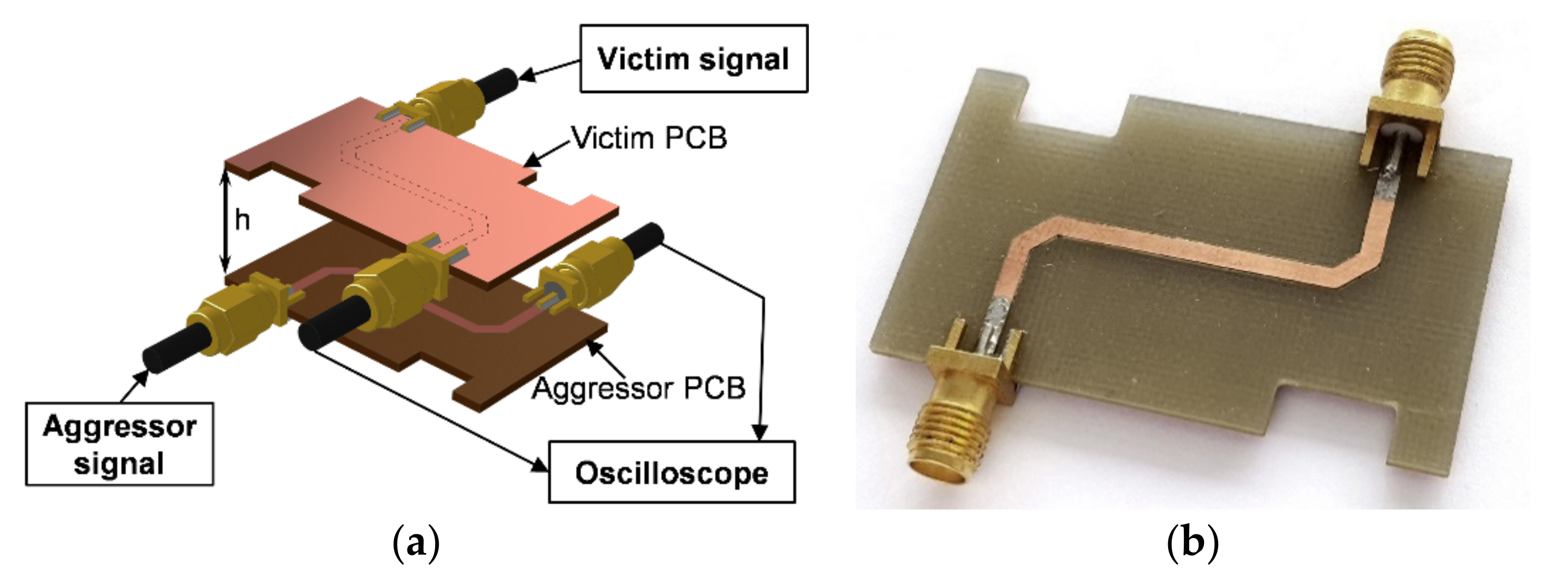
The verification of performance characteristics can be realized by simulation using the electronic design automation (EDA) software [6,7] or a direct measurement using the pseudo-random bit sequence (PRBS) generator and digital oscilloscope [8]. The complex electromagnetic compatibility (EMC) research of the high-speed data transmission link combines the time-domain measurements of the signals in the transmission lines and near-field measurements of radiated emissions [11]. The multichannel measurement setup provides simultaneous capturing of waveforms in parallel high-speed data transferring busses.

The bit error rate (BER) can be estimated by statistical processing of the measured or simulated waveforms. Traditionally in communications, performance is characterized by the parameter of the BER defined as the relative frequency of the error:

$$BER=\underset{n_{Tot}\to \infty }{\lim }\frac{n_{Err}}{n_{Tot}}$$

(1)

where $n_{Err}$ is the number of bit errors in the received data, $n_{Tot}$ is the total number of transmitted bits. The BER parameter is essentially the probability of the bit error induced by the noise and interference accompanying the process of data transferring. The BER plot shows the eye diagram opening for different sampling phases during the unit interval [12].

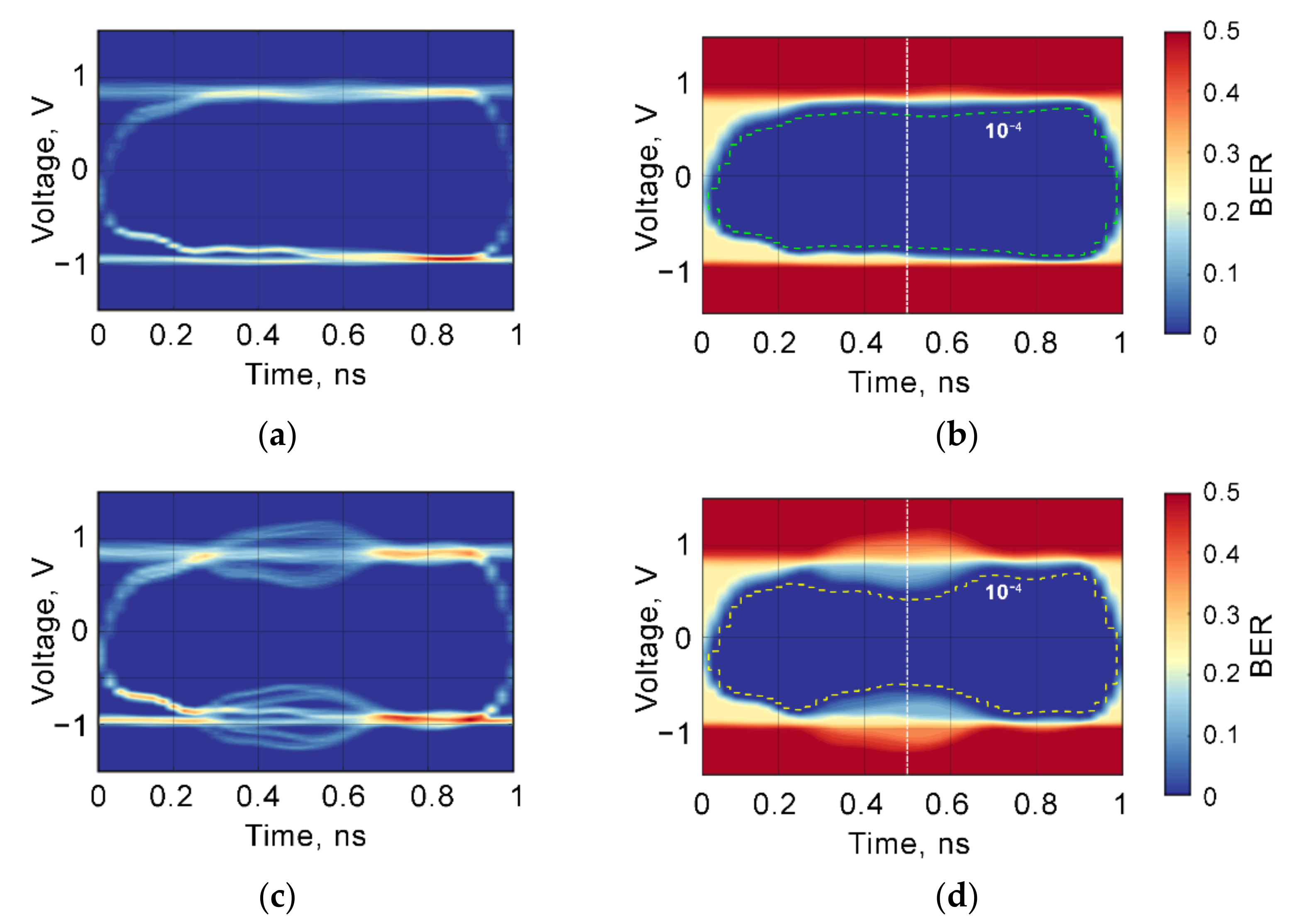
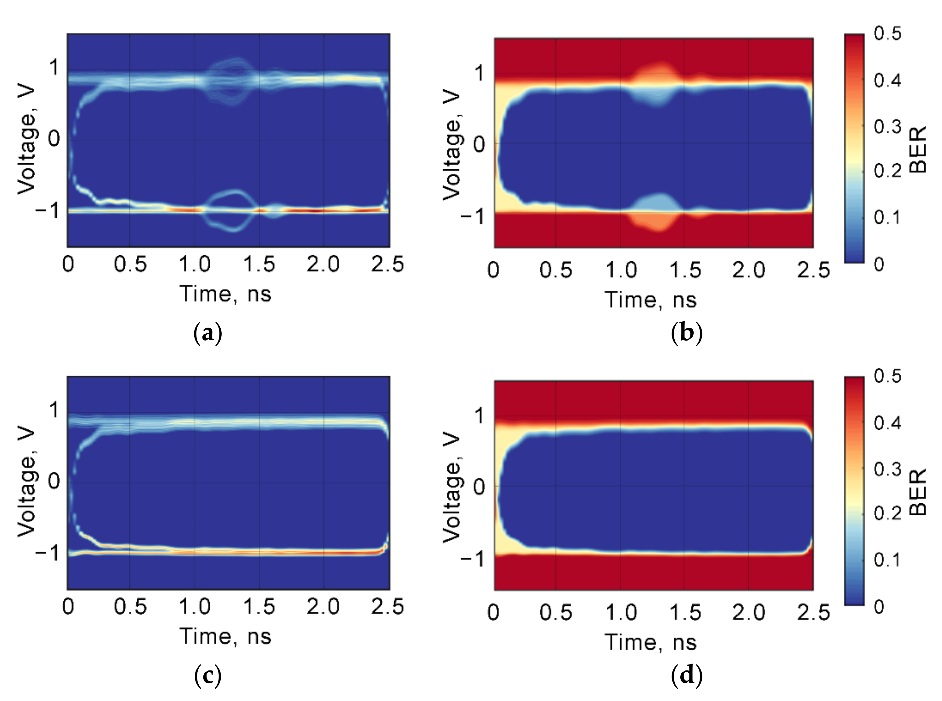
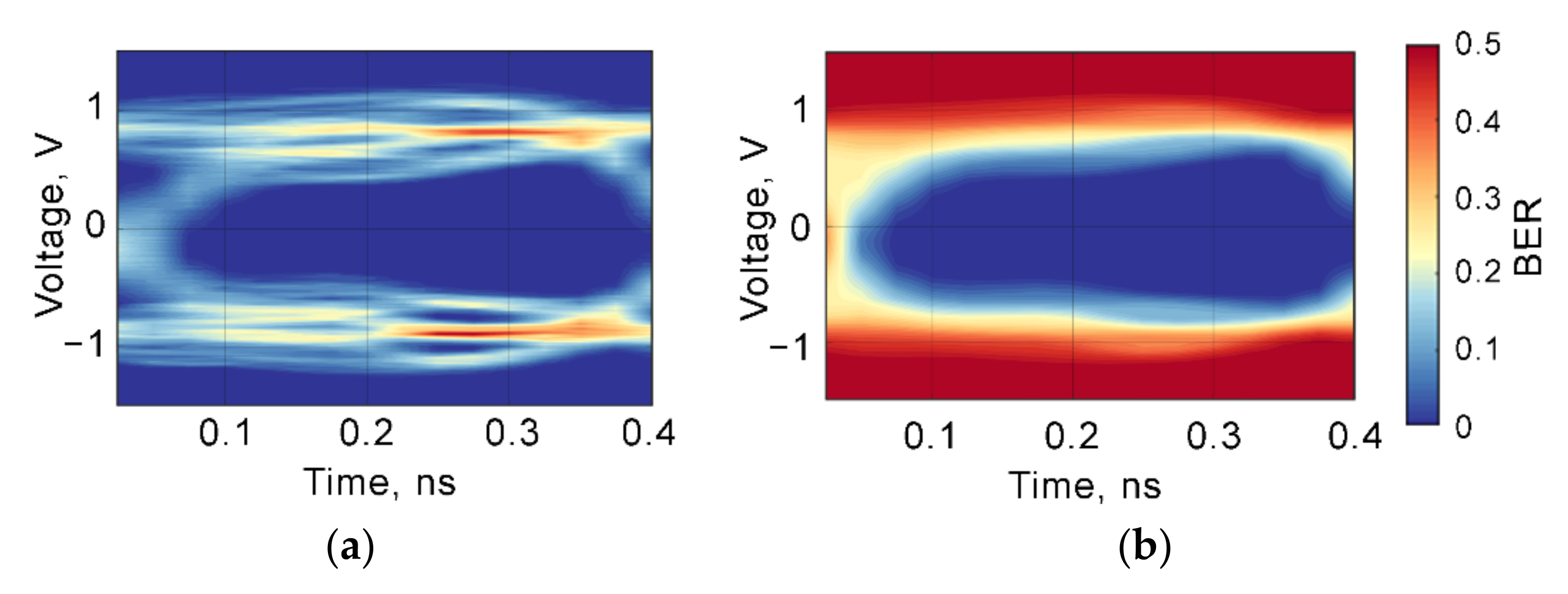
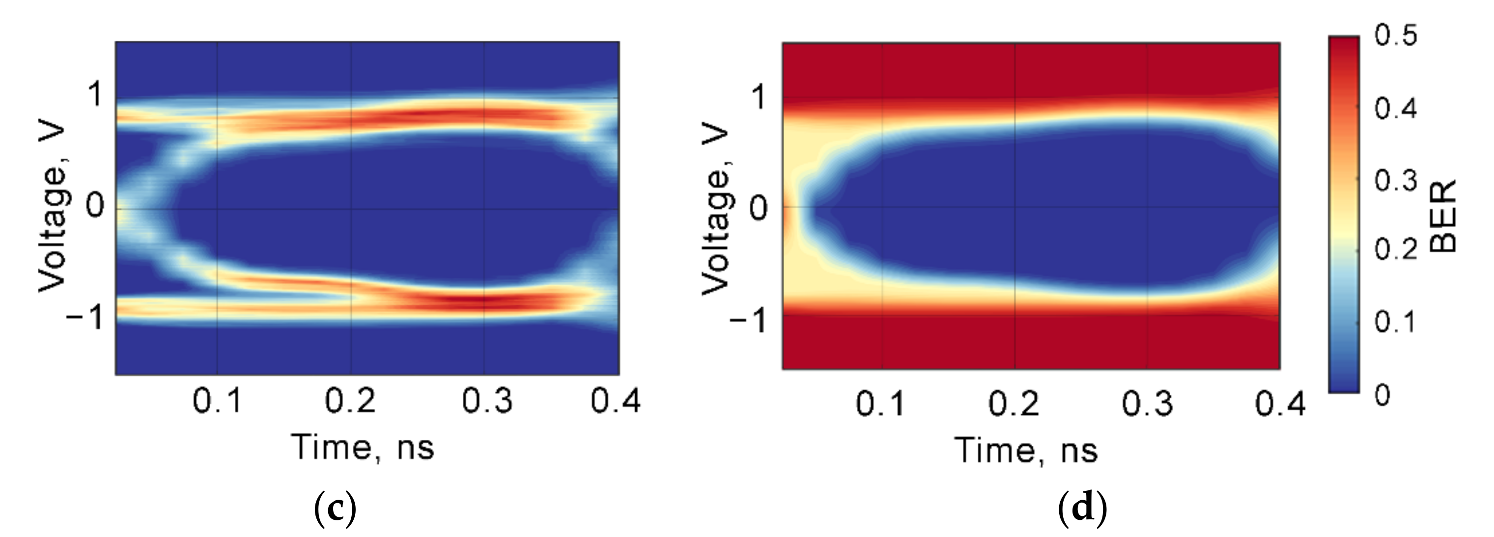
The Figure 1 shows an example of the ordinary statistical processing of waveforms with bit rate 1 Gbit/s captured using the digital oscilloscope [13]. The synchronous ensemble of cyclostationary signals can be represented by eye diagrams. Figure 1a,c present eye diagrams of measured signals without and with crosstalk interference, respectively, for the possible sampling phase during the unit interval with the duration of 1 ns. The crosstalk degrades the signal waveform decreasing the eye-opening width in the middle of the eye diagram. The corresponding BER plots are shown in Figure 1b,d. These plots show the quantity of eye-opening width for the given BER level. The green and yellow contours margin the BER level 10⁻⁴ for all sampling phases. The log-scaled BER plot can be viewed using a cross-section for the sampling phase corresponding to the middle of the signal bit response (white dash-dot vertical line).

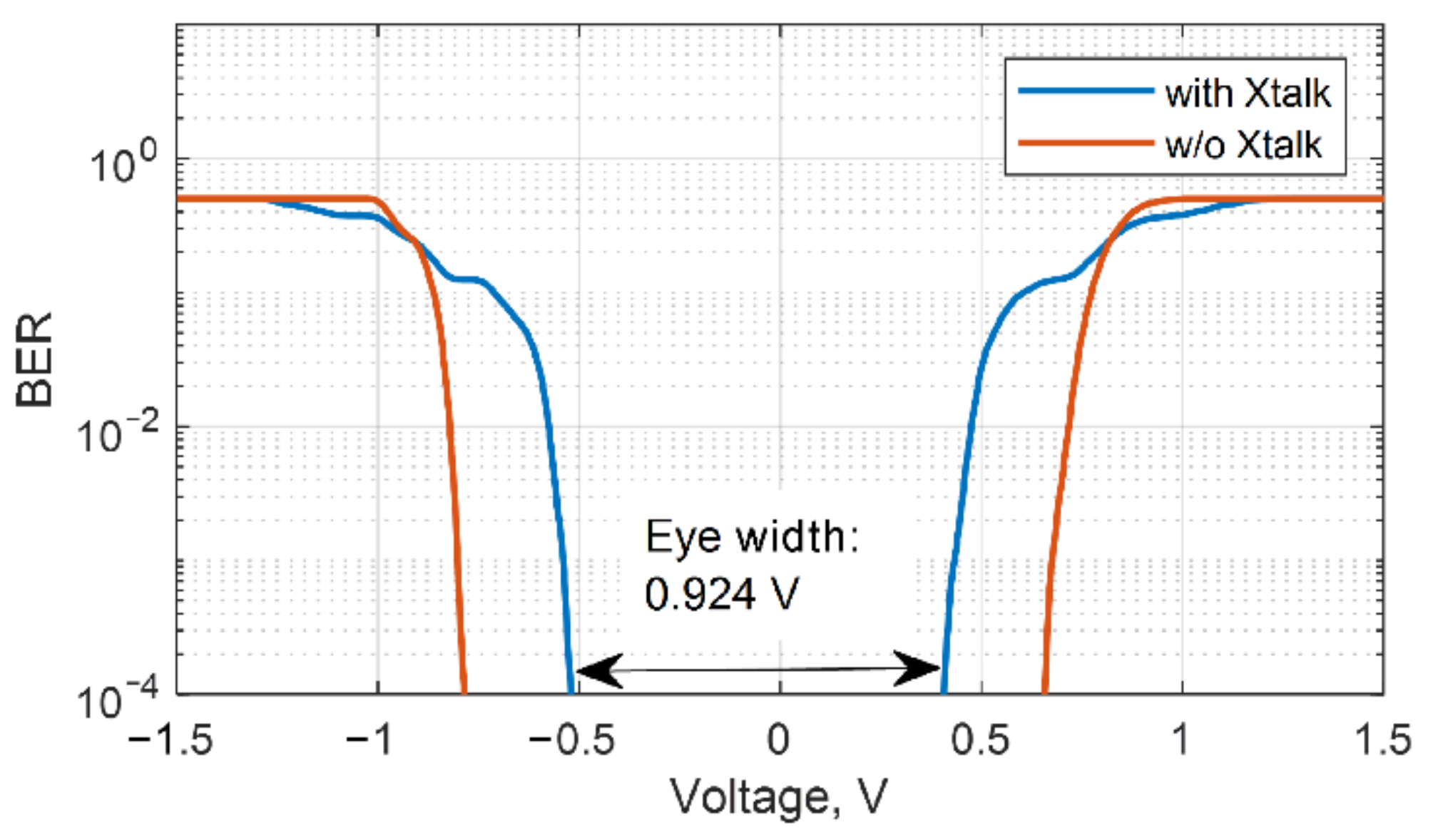
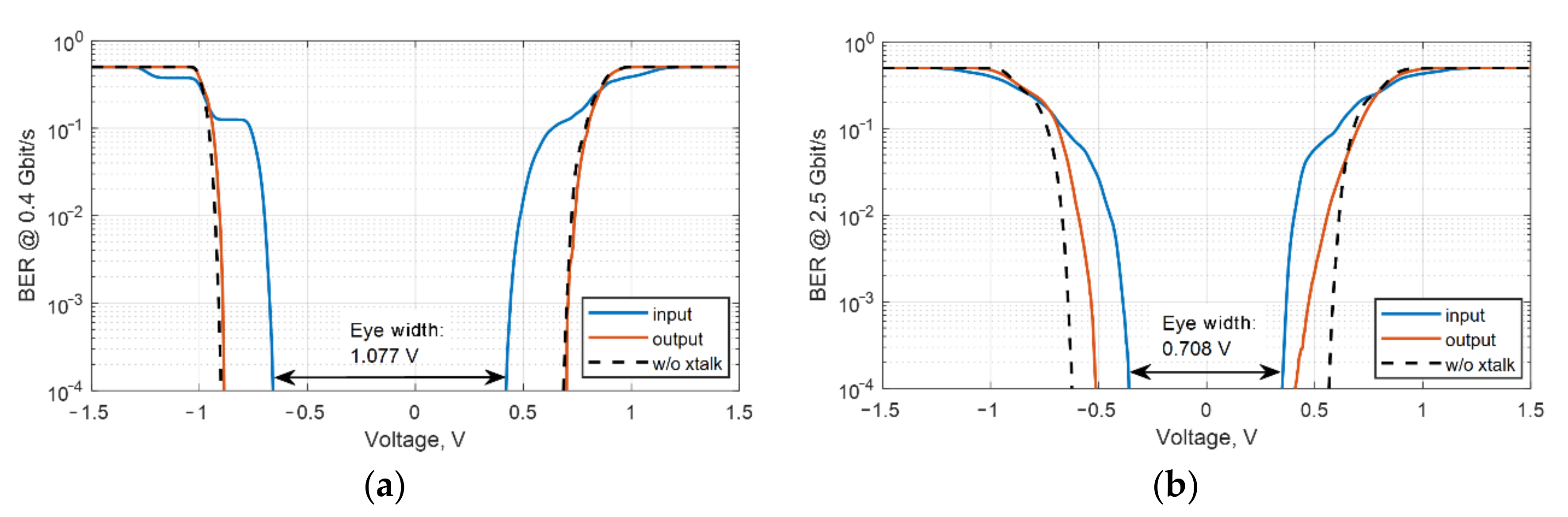
Figure 2 shows the comparison of the BER plots for signals without and with crosstalk interference [14]. The eye-opening width for the signal with crosstalk is 0.924 V.

The characterization based on the BER for the estimated signals using the minimum mean square error criterion is demonstrative for the performance comparison. In practice the reference level for the chosen figure of merit is provided by signal without crosstalk. The framework of the virtual two channel experiment without and with crosstalk is used for the synthesis and analysis of the signal estimation algorithm.

Principal component analysis (PCA) is used to investigate the measured data. The principal components can be computed by performing an eigenvalue decomposition of the data correlation matrix. The crosstalk cancelation can be viewed through the cyclostationary signal minimum MSE estimation. The key factor of the estimation is the evaluated principal components of the victim signal and crosstalk using measured data. The principal components can be expressed as single bit responses [7,8] of cyclostationary sources for the unit interval.

The estimation of measured waveforms is performed by using the cyclic Wiener filter. The principle of orthogonality provides an optimum estimator for random cyclostationary signals [15]. The cyclic Wiener filter is realized as a linear periodic time-varying filter.

The statistical signal processing of measured data can be performed using several techniques. The sliding window filtering of discrete-time signals is equivalent form of the frequency shift filtering (FRESH) [10,16]. It can be shown that simple matrix form of sliding window filtering corresponds to the multi-input to multi-output linear time-invariant transforms of the frequency shifted components of the signal.

The serial to parallel transformation of the cyclostationary signals for sliding window filtering can be viewed as forming of a stationary vector. The modern description of synthesis and analysis of signal estimators is presented using a matrix transformation of extended correlation matrices.

The paper is organized as follows. After a short introduction, the fundamentals of linear periodic time-varying filtering theory (LPTV) are provided in Section 2. The description includes frequency shifting with subsequent linear time invariant filtering (FRESH) and sliding window (SW) filtering implemented by serial to parallel transformation of the measured time series. The equivalence of both approaches is shown, and compact matrix form of the SW filtering is provided. The implementation of the cyclic Wiener filtering algorithm using the LPTV SW approach for the estimation of the input random cyclostationary data sequence corrupted by random cyclostationary crosstalk with the same cyclic period and stationary interference signals are discussed Section 3. The Wiener solution of the estimation problem is based on the principle of orthogonality, assuming the independence between the random processes constituting the measured data sequence. The independence of crosstalk and the informative cyclostationary processes can be justified by the independence of the information bit sequences in communication lines. 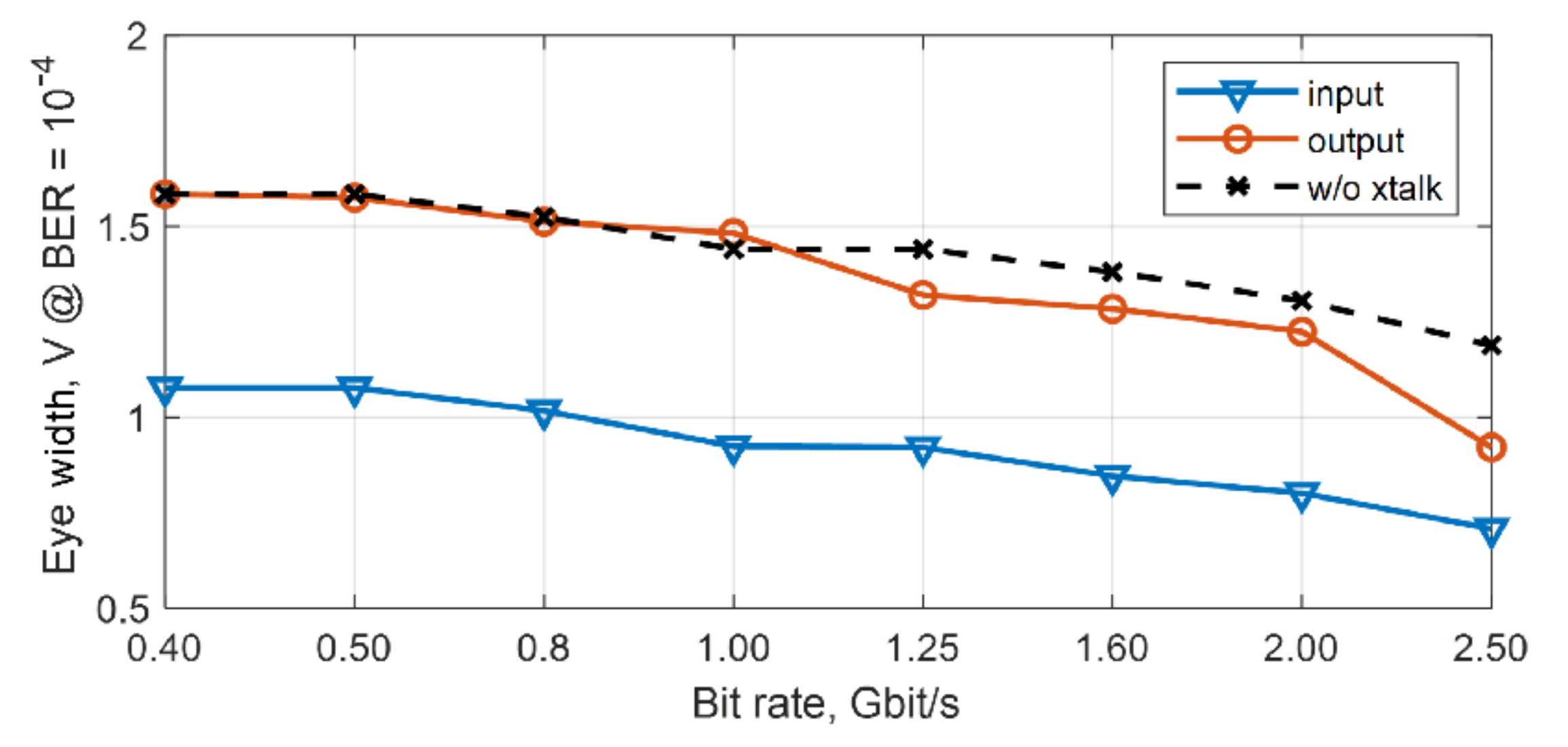The experimental research of the influence of the crosstalk from adjacent transmission line on the quality of the data communication link with and without the proposed Wiener filtering algorithm is investigated in Section 4. The quality of the data transferring is characterized by the BER related to the eye-opening width for bit rates from 0.4 Gbit/s to 2.5 Gbit/s. The paper is concluded by a discussion of obtained results.

2. Linear Periodic Time-Varying Filtering

Linear time-varying (LTV) systems are described by a wider class of signal processing algorithms than linear time invariant (LTI) systems. The filtering, modulation, compensation, equalization, and compression is representing application examples of LTV systems [16]. The superposition principle of the LTV system is very useful for statistical signal processing. The correlation analysis for LTV filtering of the additive mixture of signals, which contains a desired signal, interferences and noise, can be simplified due to the linear combination of partial output signals.

The LTV system with periodic impulse response (IR) can be used for realization of the efficient cyclostationary signal estimator known as the cyclic Wiener filter [17] (pp. 240–266). In Section 2.1, the theory of discrete-time LPTV filtering is introduced. In Section 2.2, the synthesis and analysis of the cyclic Wiener filter are discussed.

2.1. Frequency Shift Filtering

The output signal of the discrete-time LPTV system can be obtained using the following general expression

$$y(n)={\displaystyle \sum _{m=-\infty }^{\infty }h(n,m)x(m)}$$

(2)

where $x(m)$ is an input signal of the LPTV system;

$$h(n,m)=h(n+kN,m+kN)$$

(3)

is a periodic two-dimensional IR with period N.

The LPTV filtering procedure can be described particularly as frequency shifting and subsequent linear time invariant filtering [16]. The harmonic series representation (HSR) of the signals is used for such description. When $N$ is a cyclic period of the random cyclostationary process, the harmonic series decomposition provides wide sense stationary components. The equivalent LTI multi-input to multi-output (MIMO) transformation of the components is used for filtering of the overlapping in the frequency domain desired signal and interferences with the corresponding bandwidths [10].

The discrete Fourier transform (DFT) of L samples of the input signal is defined by

$$X(m)=\frac{1}{L}{\displaystyle \sum _{n=0}^{L-1}{F}_L^{-nm}x(m)}$$

(4)

where $F_L=e^{j2\pi /L}$.

The frequency shifting of the input signal by $\mu \frac{L}{N}$ and the following linear time invariant filtering using rectangular frequency response $\Pi (m)$ is expressed in the frequency domain as follow:

$${\tilde{X}}_{\mu }(m)=X\left(m+\mu \frac{L}{N}\right)\Pi (m),\mu =0,\dots ,N-1$$

(5)

where

$$\Pi (m)=U(m)-U\left(m-\frac{L}{N}\right)$$

(6)

$U(m)$ is a unit step function.

The time domain response is written using inverse DFT:

$${\tilde{x}}_{\mu }(n)={\displaystyle \sum _{m=0}^{L-1}{F}_L^{nm}{\tilde{X}}_{\mu }(m)}$$

(7)

The initial signal can be written using harmonic series representation that is the summation of the orthogonal components:

$$x(n)={\displaystyle \sum _{\mu =0}^{N-1}{F}_N^{\mu n}{\tilde{x}}_{\mu }(n)}$$

(8)

where $F_N=e^{j2\pi /N}$.

The single component of the output signal can be obtained using the equivalent discrete-time multi-input to single output (MISO) LTI filtering:

$${\tilde{y}}_{\nu }(n)={\displaystyle \sum _{\mu =0}^{N-1}{\displaystyle \sum _{m=-\infty }^{\infty }{G}_{\nu \mu }(n-m){\tilde{x}}_{\mu }(m)}}={\displaystyle \sum _{\mu =0}^{N-1}{G}_{\nu \mu }(n)\ast {\tilde{x}}_{\mu }(n)}$$

(9)

where the convolution operation is denoted by symbol ∗. The $\nu$th Fourier coefficient of the discrete time two-dimensional function$g_{\mu }(n^{\prime },n)$ is given by

$$G_{\nu \mu }(n)=\frac{1}{N}{\displaystyle \sum _{n^{\prime }=0}^{N-1}{g}_{\mu }(n^{\prime },n)F_N^{-\nu n^{\prime }}}$$

(10)

where $g_{\mu }(n^{\prime },n)$ is periodic along time $n^{\prime }$ and non-periodic along time $n$. The function $g_{\mu }(n^{\prime },n)$ can be obtained by changing variables $n=n^{\prime }$ and $m=n^{\prime }-n$ in the periodic two-dimensional IR $h_{\mu }(n,m)$ that is the μth version of the IR $h(n,m)$ frequency shifted by $\mu \frac{L}{N}$:

$$g_{\mu }(n^{\prime },n)=g_{\mu }(n^{\prime }+kN,n)=h_{\mu }(n^{\prime },n^{\prime }-n)$$

(11)

where

$$h_{\mu }(n,m)=h_{\mu }(n+kN,m+kN)=h(n,m)F_N^{\mu m}$$

(12)

The resulting output of the LPTV system is written as combination of the orthogonal components:

$$y(n)={\displaystyle \sum _{\nu =0}^{N-1}{F}_N^{\nu n}{\tilde{y}}_{\nu }(n)}$$

(13)

2.2. Sliding Window Filtering

The sliding window filtering is another efficient realization of the LPTV system for overlapped in the time domain desired signal and interferences [12]. The serial to parallel (s/p) transformation [10] of the time series can be used for SW filtering. The benefit of s/p representation is provided by the developed matrix mathematics.

The discrete-time LPTV sliding window filtering with length $N$ can be expressed using the simultaneous time shift of both the output and input signals by $kN$ and the property of the periodic two-dimensional IR:

$$y(n+kN)={\displaystyle \sum _{m=0}^{N-1}h(n+kN,m+kN)x(m+kN)}={\displaystyle \sum _{m=0}^{N-1}h(n,m)x(m+kN)}$$

(14)

The compact matrix form of the expression (14) can be obtained using s/p transformation of signal $y(n)$ to the vector signal $y[k]$:

$$\begin{array}{cc}y[k]& ={\displaystyle \sum _{n=0}^{N-1}y(n+kN)u_n}={\displaystyle \sum _{n=0}^{N-1}{u}_n}{\displaystyle \sum _{m=0}^{N-1}h(n,m)x(m+kN)}\hfill \\ & ={\displaystyle \sum _{n=0}^{N-1}{\displaystyle \sum _{m=0}^{N-1}{u}_{n}h(n,m)u_m^{T}x(m+kN)u_m}}=Hx[k], k=0,\dots ,\frac{L}{N}-1\hfill \end{array}$$

(15)

where

$$H={\displaystyle \sum _{n=0}^{N-1}{\displaystyle \sum _{m=0}^{N-1}{u}_{n}h(n,m)u_m^T}}\mathbf{ }$$

(16)

$$x[k]={\displaystyle \sum _{m=0}^{N-1}x(m+kN)u_m}\mathbf{ }$$

(17)

$$u_m=P^m{u}_0$$

(18)

is mth unit vector obtained by $m$ permutations of the initial unit vector $u_0={(1 0 \dots 0)}^T$;

$$P=\left(\begin{array}{cccc}0& 0& \cdots & 0\\ 1& 0& \ddots & ⋮\\ ⋮& \ddots & 0& 0\\ 0& \cdots & 1& 0\end{array}\right)$$

(19)

is a permutation matrix.

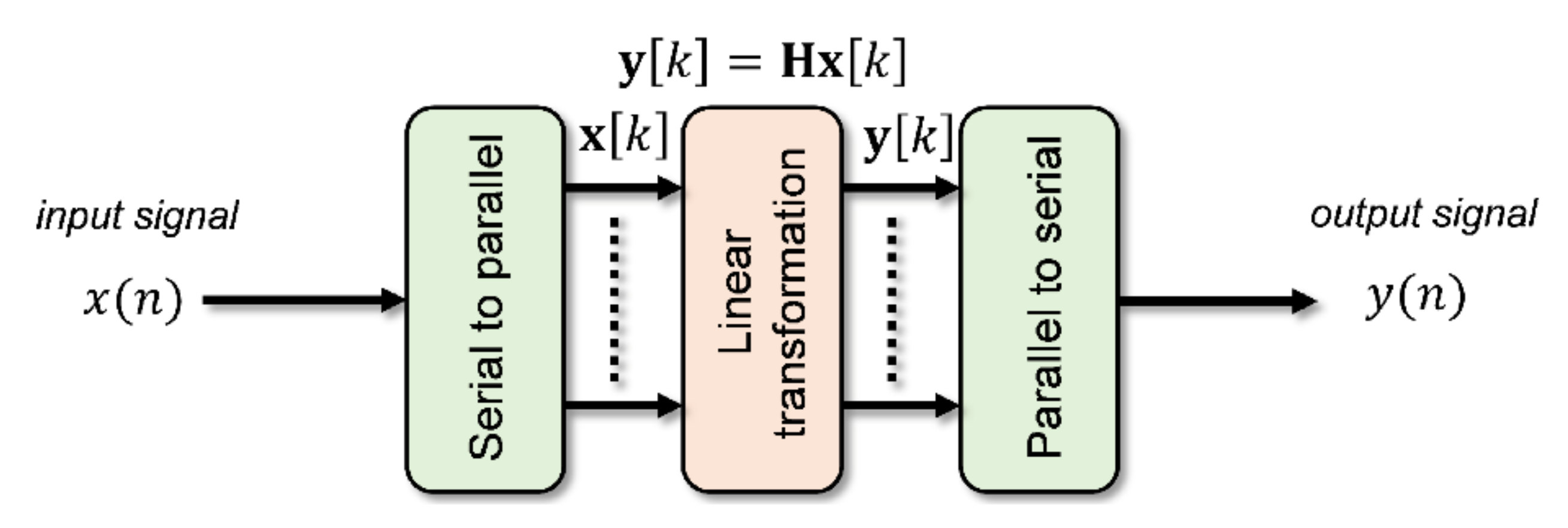
The scheme of SW filtering is shown in Figure 3. It consists of the s/p transformation of the input signal $x\left(n\right)$, linear transformation (15) of the parallel vector signal $x\left[k\right]$ and parallel to serial (p/s) transformation of the parallel vector signal $y\left[k\right]$ for obtaining the output serial signal $y\left(n\right)$.

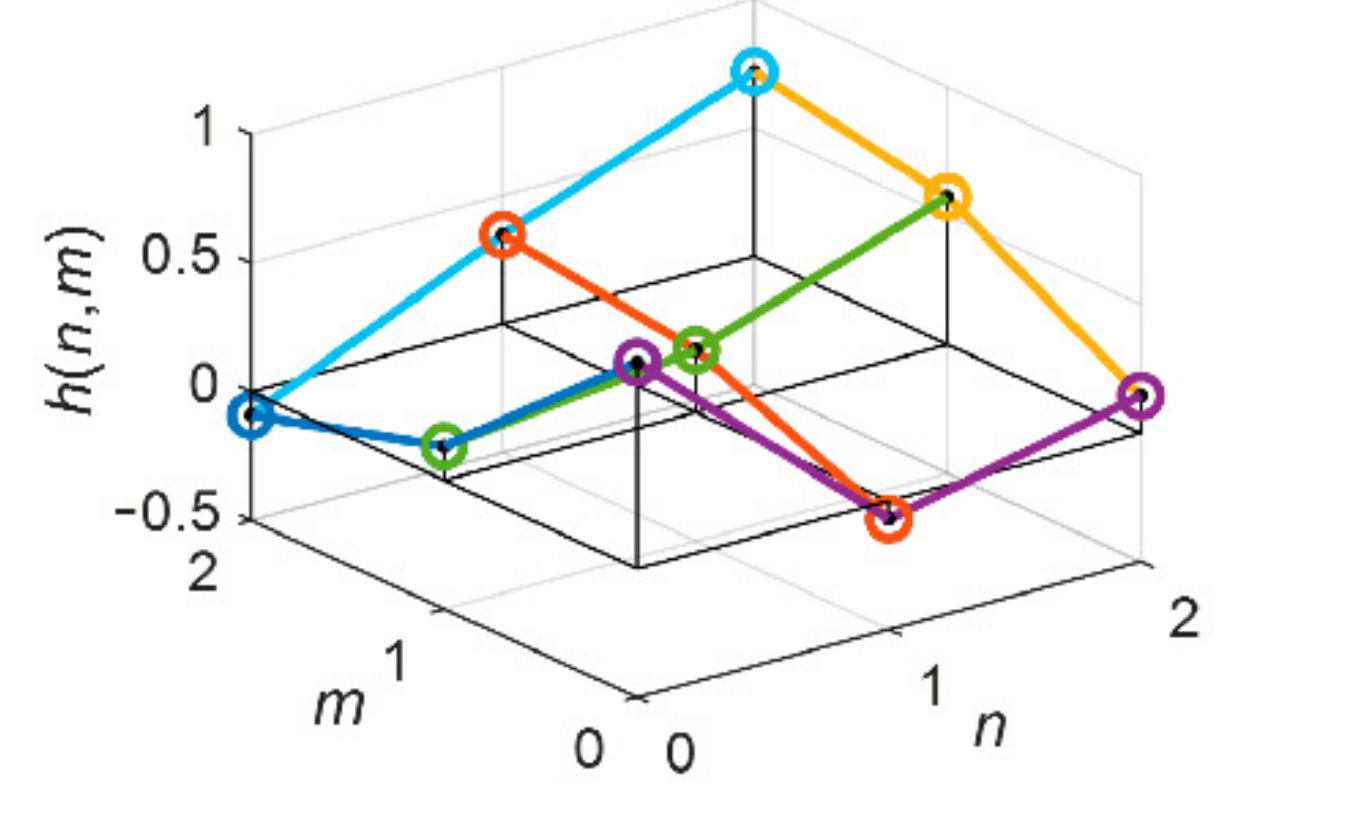
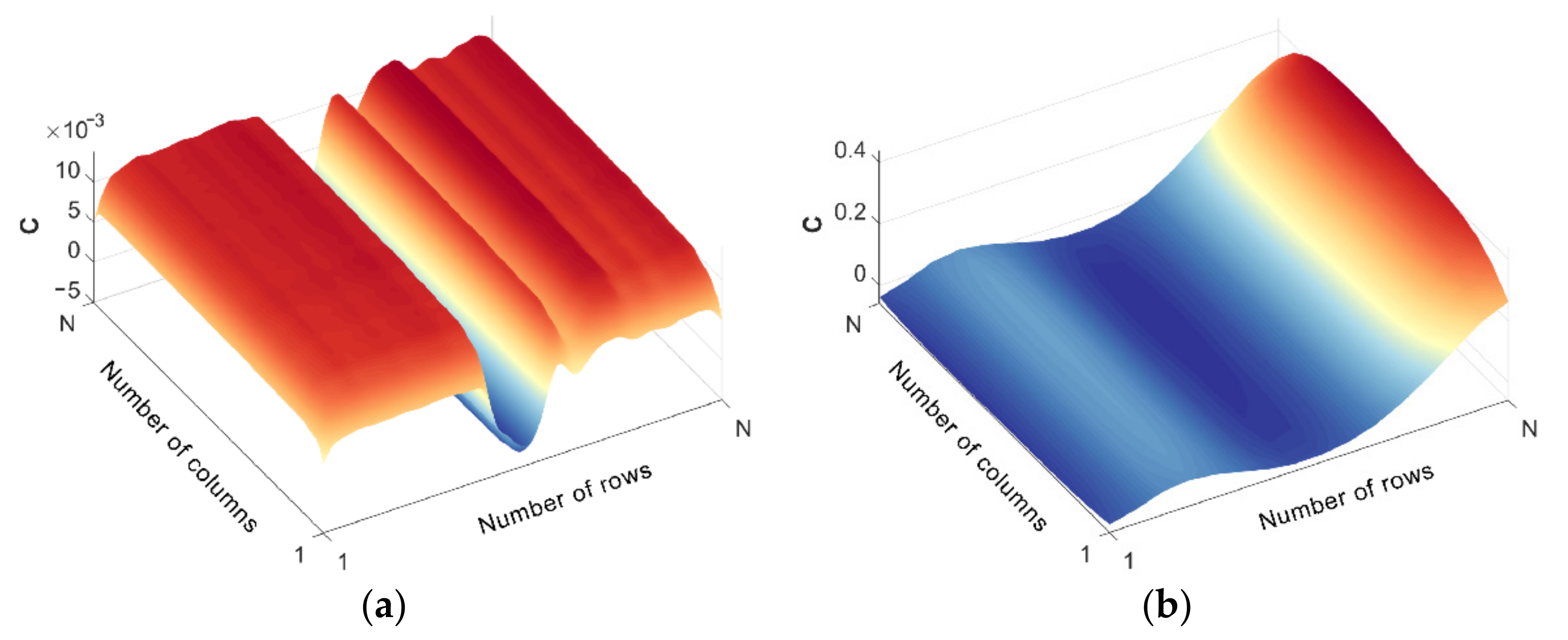
An example of a two-dimensional impulse response $h\left(n,m\right)$ of an SW filter is shown in Figure 4. The chosen number of samples per cyclic period $N=3$.

The relation between the equivalent FRESH and SW type of LPTV filtering can be obtained through s/p transformation for the corresponding HSR components of the input and output signals:

$$x[k]={\displaystyle \sum _{n=0}^{N-1}x(n+kN)u_n}={\displaystyle \sum _{\mu =0}^{N-1}{F}^{\mu }{\tilde{x}}_{\mu }[k]}, y[k]={\displaystyle \sum _{n=0}^{N-1}y(n+kN)u_n}={\displaystyle \sum _{\nu =0}^{N-1}{F}^{\nu }{\tilde{y}}_{\nu }[k]}\mathbf{ }$$

(20)

where

$${\tilde{x}}_{\mu }[k]={\displaystyle \sum _{n=0}^{N-1}{\tilde{x}}_{\mu }(n+kN)u_n}, {\tilde{y}}_{\nu }[k]={\displaystyle \sum _{n=0}^{N-1}{\tilde{y}}_{\nu }(n+kN)u_n},F=\mathrm{diag}(0,\hspace{0.33em}{F}_N, \dots , F_N^{N-1})$$

(21)

The FRESH filtering also has the following compact matrix form:

$$\begin{array}{cc}\tilde{y}(n)& ={\displaystyle \sum _{\nu =0}^{N-1}{\tilde{y}}_{\nu }(n)u_{\nu }}={\displaystyle \sum _{\nu =0}^{N-1}{\displaystyle \sum _{\mu =0}^{N-1}{u}_{\nu }{G}_{\nu \mu }(n)\ast {\tilde{x}}_{\mu }(n)}}\hfill \\ & ={\displaystyle \sum _{\nu =0}^{N-1}{\displaystyle \sum _{\mu =0}^{N-1}{u}_{\nu }{G}_{\nu \mu }(n)u_{\mu }^T\ast {\tilde{x}}_{\mu }(n)u_{\mu }}}=G(n)\ast \tilde{x}(n)\hfill \end{array}$$

(22)

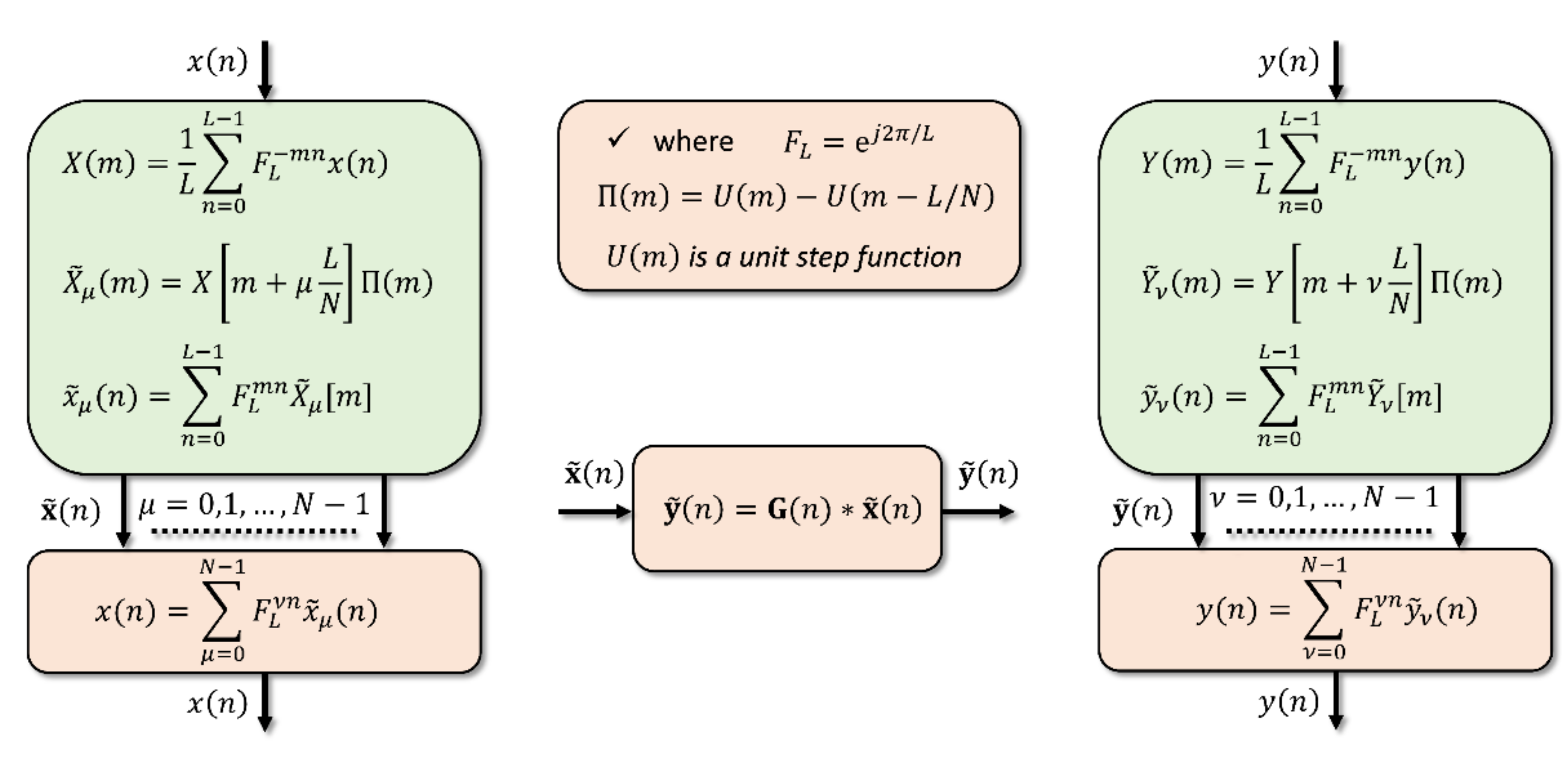
where the convolution operation is denoted by symbol ∗,

$$G(n)={\displaystyle \sum _{\nu =0}^{N-1}{\displaystyle \sum _{\mu =0}^{N-1}{u}_{\nu }{G}_{\nu \mu }(n)u_{\mu }^T}}, \tilde{x}(n)={\displaystyle \sum _{\mu =0}^{N-1}{\tilde{x}}_{\mu }(n)u_{\mu }}\mathbf{ }$$

(23)

Figure 5 shows the scheme of the frequency shift filtering. The linear transformation has the form of multi-input to multi-output filtering.

The $\nu$th Fourier coefficient of the LTI filter impulse response can be expressed using the inner product of the permutated frequency shifted matrix$H_{\mu }$ and matrix ${\Phi }^{\nu }=N^{-1}{F}^{\nu }$:

$$G_{\nu \mu }(n)=\langle H_{\mu }{P}_n,{\Phi }^{\nu }\rangle =N^{-1}\langle H_{\mu }{P}_n,F^{\nu }\rangle =N^{-1}\mathrm{tr}\left(F^{\nu H}{H}_{\mu }{P}_n\right)$$

(24)

where $H_{\mu }=H{F}^{\mu }$ is a frequency shifted version of the matrix $H$,

$$P_n=\{\begin{array}{c}{P}^{nT},0\le n\le N-1\hfill \\ P^{\left|n\right|},-N+1\le n<0\hfill \end{array}$$

(25)

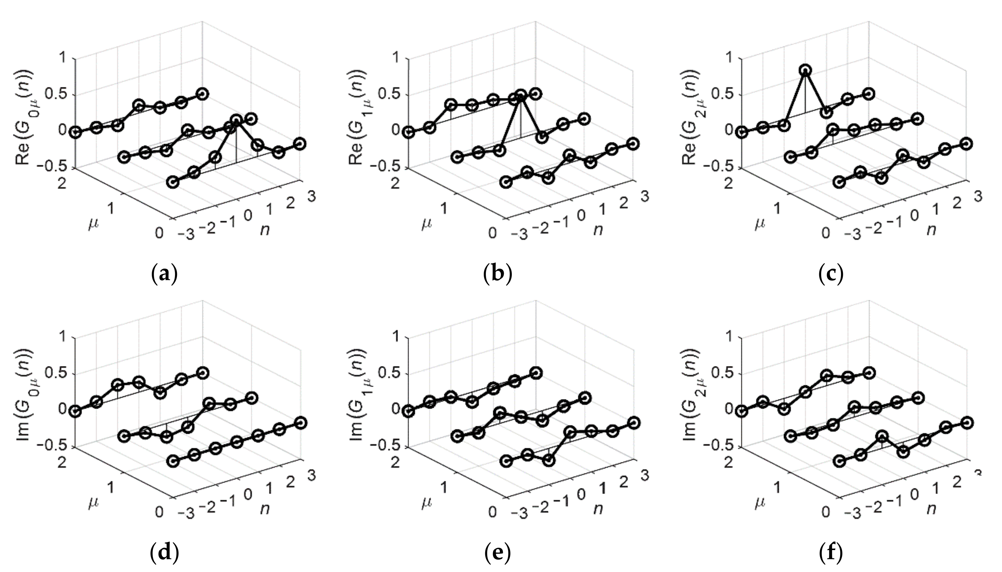
The bank of one-dimensional IRs of the FRESH filter is shown in Figure 6. This structure is functionally equivalent to the SW filter with a two-dimensional IR shown in Figure 4. The single one-dimensional IR is complex valued. Real parts are shown in Figure 6a–c. The corresponding imaginary parts are presented in Figure 6d–f.

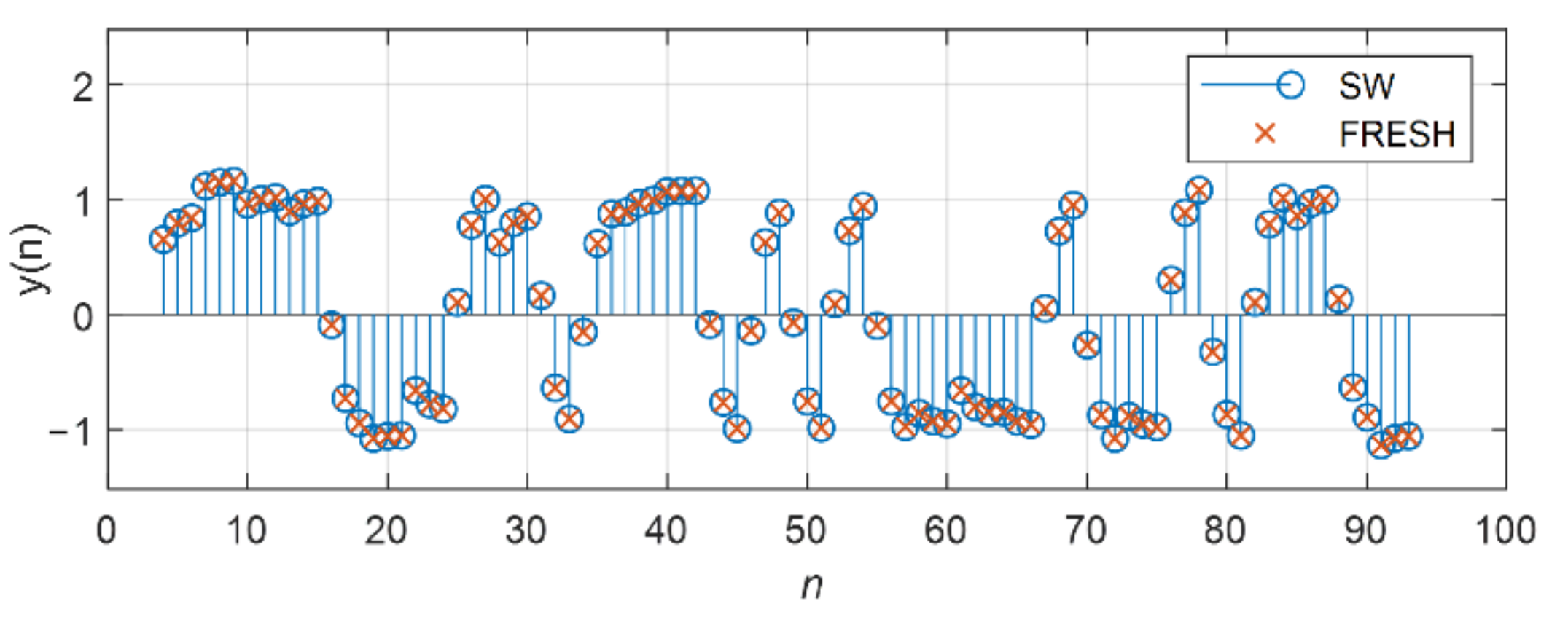
The transformation of signal in the LPTV system can be realized by SW filtering or by equivalent FRESH filtering. An example of the output pulse amplitude modulated (PAM) signal is shown in Figure 7 for both types of filters.

The analysis of the compact matrix form of the SW LPTV filtering using HSR shows that its FRESH representation includes frequency shifts and MIMO LTI filtering of band-limited components of the input signal. The output full-band signal is obtained by combining the orthogonal components.

3. Synthesis and Analysis of Cyclic Wiener Filter

The signal estimation problem can be viewed through the SW filtering of the measured signals rearranged using serial to parallel transformation. This estimator is referred as a Wiener filter. The equality of the period of the corresponding LPTV filter and cyclic period of the corresponding random cyclostationary processes makes the estimator a cyclic Wiener filter.

The matrix notation used for the SW filtering of cyclostationary signals simplifies the description dealing with the stationary vectors. The desired signal is transformed into a real-valued vector $x\left[k\right]$. The measured signal denoted by the vector $y\left[k\right]$ with the same length is linear transformed using a real-valued weighting matrix $W$. The difference between estimated and desired signals is an estimation error $e\left[k\right]$. Two equations can be used for the introduction of the signal estimation problem, avoiding denotation of the filter output signal:

$$\begin{array}{l}x[k]=Wy[k]-e[k]\\ e[k]=Wy[k]-x[k]\end{array}$$

(26)

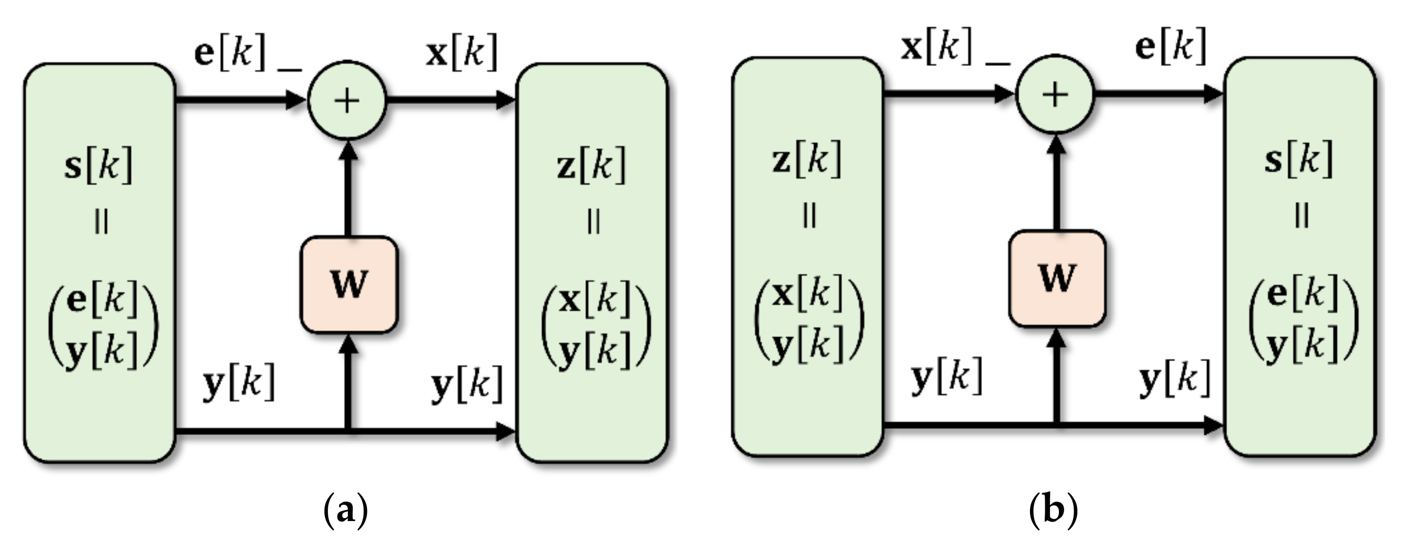
The obtained dual equations can be mapped into the composite form using the virtual two channel estimation problem. Figure 8 shows the pair of two-channel systems where input and output vectors are composite block vectors. The block vector $z\left[k\right]$ is obtained as a composition of vectors $x\left[k\right]$ and $y\left[k\right]$. The block vector $s\left[k\right]$ consists of vectors $e\left[k\right]$ and $y\left[k\right]$. The scheme in Figure 8a is used for synthesis, and the scheme in Figure 8b is used for an analysis problem. The mentioned schemes are identical if permuting input and output block vectors. The motivation of this step is an application of the partitioned correlation matrices for input and output composite vectors. These matrices contain all the necessary correlations between vectors for solving estimation problems.

The input to output relations for the corresponding synthesis and analysis schemes shown in Figure 8 can be written using partitioned matrix $B$ for the definition of linear transformation of composite vectors $z\left[k\right]$ and $s\left[k\right]$ in accordance with (26) as follows:

$$\begin{array}{l}z[k]=Bs[k]=\left(\begin{array}{c}x[k]\\ y[k]\end{array}\right)=\left(\begin{array}{cc}-I& W\\ 0& I\end{array}\right)\left(\begin{array}{c}e[k]\\ y[k]\end{array}\right)\\ s[k]=Bz[k]=\left(\begin{array}{c}e[k]\\ y[k]\end{array}\right)=\left(\begin{array}{cc}-I& W\\ 0& I\end{array}\right)\left(\begin{array}{c}x[k]\\ y[k]\end{array}\right)\end{array}$$

(27)

where $I$ is an identity matrix.

The correlation matrix of the block vector $z\left[k\right]$ is a partitioned block matrix:

$$R_{zz}={\rm E}\{z[k]z^T[k]\}=\left(\begin{array}{cc}{R}_{xx}& R_{xy}\\ R_{yx}& R_{yy}\end{array}\right)$$

(28)

where ${\rm E}\{•\}$ is an expectation operator, $R_{xx}={\rm E}\left\{x[k]x^T[k]\right\}$ and $R_{yy}={\rm E}\left\{y[k]y^T[k]\right\}$ are the correlation matrices; $R_{xy}={\rm E}\left\{x[k]y^T[k]\right\}$ and $R_{yx}={\rm E}\left\{y[k]x^T[k]\right\}$ are the cross-correlation matrices.

The Wiener solution of the estimation problem is based on the principle of orthogonality. The error $e\left[k\right]$ and the measurement $y\left[k\right]$ are the uncorrelated random signals so that:

$${\rm E}\left\{e[k]y^T[k]\right\}={\rm E}\left\{y[k]e^T[k]\right\}=0$$

(29)

The correlation matrix of composite vector $s\left[k\right]$ is analyzed in the same manner as the correlation matrix $R_{zz}$ and has a block diagonal form due to the orthogonality of the error and measured signal:

$$R_{ss}={\rm E}\{s[k]s^T[k]\}=\left(\begin{array}{cc}Q& 0\\ 0& R_{yy}\end{array}\right)$$

(30)

where

$$Q={\rm E}\left\{e[k]e^T[k]\right\}\mathbf{ }$$

(31)

is an error covariance matrix.

The linear transformation of the random composite vectors $s\left[k\right]$ and $z\left[k\right]$ for synthesis and analysis schemes can be viewed through the transformation of corresponding correlation matrices using matrix $B$:

$$\begin{array}{l}{R}_{ss}=B{R}_{zz}B=\left(\begin{array}{cc}-I& W\\ 0& I\end{array}\right)\left(\begin{array}{cc}{R}_{xx}& R_{xy}\\ R_{yx}& R_{yy}\end{array}\right)\left(\begin{array}{cc}-I& 0\\ W^T& I\end{array}\right)\\ R_{zz}=B{R}_{ss}B=\left(\begin{array}{cc}-I& W\\ 0& I\end{array}\right)\left(\begin{array}{cc}Q& 0\\ 0& R_{yy}\end{array}\right)\left(\begin{array}{cc}-I& 0\\ W^T& I\end{array}\right)\end{array}$$

(32)

The upper triangular matrix $U$ and block diagonal matrix $D$ corresponding to the Cholesky decomposition of partitioned correlation matrix $R_{zz}$ can be used for matrix factorization:

$$R_{zz}=UD{U}^T=\left(\begin{array}{cc}I& R_{xy}{R}_{yy}^{-1}\\ 0& I\end{array}\right)\left(\begin{array}{cc}{R}_{zz}/R_{yy}& 0\\ 0& R_{yy}\end{array}\right)\left(\begin{array}{cc}I& 0\\ R_{yy}^{-1}{R}_{yx}& I\end{array}\right)$$

(33)

where

$$R_{zz}/R_{yy}=R_{xx}-R_{xy}{R}_{yy}^{-1}{R}_{yx}$$

(34)

is the Schur complement of $R_{yy}$ in $R_{zz}$.

The comparison the blocks $U$ in (33) and $B$ in (32) gives the equation for the cyclic Wiener filter:

$$W=R_{xy}{R}_{yy}^{-1}\mathbf{ }$$

(35)

The error covariance matrix $Q$ can be found by comparing correlation matrix $R_{ss}$ in (32) and block diagonal matrix $D$ in (33):

$$Q=R_{zz}/R_{yy}=R_{xx}-R_{xy}{R}_{yy}^{-1}{R}_{yx}$$

(36)

In summary of this section, the virtual two channel experiments can be discussed. The analysis problem corresponds to the linear transformation of composite vector $z[k]$.

This model produces an error that is orthogonal to the measurement provided by the appropriate Wiener filter. The synthesis problem can be modeled using the same linear transformation of the composite vector $s[k]$ with a given block diagonal correlation matrix that returns the vector $z[k]$. The decomposition of the correlation matrix of vector $z[k]$ provides the block Cholesky factors corresponding to the transformed correlation matrix of vector $s[k]$.

The crosstalk interference canceler is a specific cyclic Wiener filter. The main contribution to the disturbance of the signal is generated by cyclostationary crosstalk in the presence of low stationary noise compared with the desired signal. The characteristics of the synthesized and analyzed cyclic Wiener filters for crosstalk cancelation is presented in Section 4.

4. Experimental Results

4.1. Measurement Setup

The measurements of electromagnetic emissions caused by the data sequence transferred along transmission line in the presence of crosstalk interference were implemented by the test setup shown in Figure 9. The binary PRBS with the length equal to (2¹⁰–1) binary symbols was generated by the Anritsu pulse pattern generator MP1604B.

The wiring diagram of the measurement equipment is presented in Figure 9a. Two identical microstrip lines of zigzag configuration were placed in parallel with 1 mm between them. One line was assumed as a victim and the other one as the aggressor. Microstrip lines were fed by the same Anritsu pulse pattern generator, but the aggressor’s sequence was delayed by some random time duration for eliminating the correlation between PRBSs. Microstrip lines were fabricated using a 1.6 mm thick FR4 substrate with a characteristic impedance of 50 Ω having the length of 50 mm and the width of 1.85 mm. The photo of the microstrip line is shown in Figure 9b.

Synchronous measurement of signals passing through the transmission lines were implemented by a serial data analyzer LeCroy SDA 813Zi-A with a sampling frequency of 40 GSa/s. The total number of samples registered in each realization for implementing the ensemble averaging procedure was chosen around five million, which is less than the duration of the PRBS. This allows to confirm the randomness of the registered data.

4.2. Correlation Analysis of the Measured Signals

The crosstalk voltage can be assumed as an additive and an independent component of the received signal. The aggressor’s signal transmitted in the parallel transmission line has the same cyclic period as the victim’s signal [12]. Time-domain measurement of the signals in the transmission lines can be implemented using digital oscilloscopes with sampling rates above decades of gigahertz [18]. The signals measured by real-time oscilloscope were characterized directly in the time-domain. The impulse response of the periodic filter is estimated using time-domain characteristics.

The model of the registered signal $v(n)$ in the assumption of observing the signal of interest $d(n)$ corrupted by additive interference $c(n)$ and stationary noise $w(n)$ is given by:

$$v(n)=d(n)+c(n)+w(n)$$

(37)

The correlation matrix of the measured signal $v(n)$ can be expressed as the sum of the correlation matrices $R_{dd}$, $R_{cc}$ and $R_{ww}$ for corresponding jointly uncorrelated components of the signal $v(n)$:

$$R_{vv}=R_{dd}+R_{cc}+R_{ww}=S\Sigma S^T+R_{ww}$$

(38)

where $S\Sigma S^T$ is a decomposition of the correlation matrix for cyclostationary sources using principal components; $S=(s_d s_c)$ is a composite matrix of the eigenvectors $s_d$ and $s_c$ of the correlation matrices $R_{dd}$ and $R_{cc}$, respectively; $\Sigma =\mathrm{diag}({\lambda }_d,{\lambda }_c)$ is a diagonal matrix with diagonal elements corresponding to the eigenvalues ${\lambda }_d$ and ${\lambda }_c$ of the correlation matrices $R_{dd}$ and $R_{cc}$, respectively; $R_{ww}$ is diagonal correlation matrix of wide sense stationary noise.

The crosstalk canceler can be expressed as cyclic Wiener filter using equation (35):

$$C=R_{dv}{R}_{vv}^{-1}\mathbf{ }$$

(39)

where

$$R_{dv}=R_{vd}^T=R_{dd}$$

(40)

is a cross correlation matrix of the signal of interest and the received signal;

$$R_{vv}^{-1}={\left(S\Sigma S^T+R_{ww}\right)}^{-1}=R_{ww}^{-1}-R_{ww}^{-1}S{\left({\Sigma }^{-1}+S^T{R}_{ww}^{-1}S\right)}^{-1}{S}^T{R}_{ww}^{-1}$$

(41)

is the inverse of the correlation matrix $R_{vv}$ obtained using the matrix inversion lemma or Woodbury identities [19].

The cyclic Wiener filter $C$ is the LPTV filter used for the waveform estimation of the signal of interest $d(n)$.

Figure 10 and Figure 11 show the estimated correlation matrices of the cyclostationary sources, the evaluated eigenvalues and scaled eigenvectors corresponding to first eigenvalues of correlation matrices for bit rates 0.4 Gbit/s and 2.5 Gbit/s respectively.

Figure 12 shows the cyclic Wiener filter $C$ for signals with bit rates 0.4 Gbit/s and 2.5 Gbit/s respectively.

The calculated weighting matrix $C$ for the data signal estimator has a dumped region (“canyon”) due to the peak of the crosstalk correlation matrix. Except this region, the weighting matrix repeats the flat form of the data signal correlation matrix. The signal estimation can be physically interpreted as a balanced rejection of fluctuations caused by crosstalk concentrated over time in the middle of the data signal single bit response. As a result, it achieved immunity of the output signal to the crosstalk fluctuations and the reception sufficient part of the data signal to resist the noise.

4.3. Bit Error Rate Estimation

In order to demonstrate the effectiveness of the cyclic Wiener filtering and discuss the results of the crosstalk cancelation an analysis of the eye diagrams and BER characterization was performed. Figure 13 and Figure 14 show pairs of the eye diagrams and the corresponding BER diagrams for bit rates 0.4 Gbit/s and 2.5 Gbit/s, respectively. Figure 15 shows the bit error rate versus the voltage for the middle of the single bit responses for bit rates 0.4 Gbit/s and 2.5 Gbit/s. The figures verify the effective crosstalk cancelation using the cyclic Wiener filter. However, the achieved eye-opening width is smaller for bit rate 2.5 Gbit/s than for bit rate 0.4 Gbit/s. This tendency was analyzed using a series of experiments.

The same statistical signal processing was performed for eight different bit rates from 0.4 Gbit/s to 2.5 Gbit/s:

• Correlation analysis of the signals measured by digital oscilloscope including time synchronization, correlation matrix estimation, evaluation of the eigenvalue decomposition;
• Weighting matrix calculation using the inverse correlation matrix and the following SW filtering of victim signal with crosstalk using serial to parallel transformation;
• Eye-opening width estimation in the middle of the single bit response for the BER level 10⁻⁴.

Figure 16 shows the obtained results of estimated eye-opening width for bit rates from 0.4 Gbit/s to 2.5 Gbit/s.

It can be seen in Figure 16 the degradation of the effectiveness of the performed signal estimation for increasing bit rates. The physical reason of such degradation is the decreasing in the signal to interference ratio. The mathematical interpretation is increasing the projection of the error produced by the evaluated cyclic Wiener filter to the observed measurement.

5. Conclusions

The current study focuses on the realization of the parallel high-speed data transferring busses can encounter and induce unintentional emission of crosstalk signals. The assurance of signal integrity in such data transmission links can be achieved by the crosstalk cancelation using a transceiver utilizes the cyclostationary properties of crosstalk. The model of the victim signal consists of the valuable data signal corrupted by the additive of the cyclostationary aggressor signal and stationary noise. The independence of the crosstalk and informative cyclostationary processes is justified by the independence of the information bit sequences in communication lines of the aggressor and the victim. In this case, the filtering of the observed measured random process can be implemented by the cyclic Wiener filter, estimating the message in the measured signal.

Filtering of the random process with periodical correlation properties needs to be implemented by the linear system with a periodically changing impulse response. It is shown that the output of an LPTV structure may be expressed as a sum of the filtered versions of frequency shifted copies of the input cyclostationary random process. The equivalent time-domain sliding window transformation of the cyclostationary random process assumes the serial to parallel transformation of the input signal, multi-input to multi-output linear filtering of this vector process, and the parallel to serial transformation providing the filtered cyclostationary output signal.

The experimental results obtained by cyclic averaging of the measured random processes before and after the cyclic Wiener filtering showed significant reduction in the crosstalk interference components in the estimated message signal. The evaluated eye diagrams provide the estimation of the bit error rate which quantitatively characterizes the transmission of data after the implemented filtering of the aggressor’s interference. The investigated dependence of the eye-opening width versus bit rate of the data transferring showed the reduction in the eye width caused by a decrease in the signal to interference ratio of the measured signal.