A Data-Driven Forecasting Strategy to Predict Continuous Hourly Energy Demand in Smart Buildings

Abstract

Smart buildings seek to have a balance between energy consumption and occupant comfort. To make this possible, smart buildings need to be able to foresee sudden changes in the building’s energy consumption. With the help of forecasting models, building energy management systems, which are a fundamental part of smart buildings, know when sudden changes in the energy consumption pattern could occur. Currently, different forecasting methods use models that allow building energy management systems to forecast energy consumption. Due to this, it is increasingly necessary to have appropriate forecasting models to be able to maintain a balance between energy consumption and occupant comfort. The objective of this paper is to present an energy consumption forecasting strategy that allows hourly day-ahead predictions. The presented forecasting strategy is tested using real data from two buildings located in Valladolid, Spain. Different machine learning and deep learning models were used to analyze which could perform better with the proposed strategy. After establishing the performance of the models, a model was assembled using the mean of the prediction values of the top five models to obtain a model with better performance.

1. Introduction

Energy consumption forecasting models have become a fundamental piece of smart buildings to develop energy efficiency for a sustainable economy [1]. Forecasting models learn the utilization patterns from the chronicled energy consumption information to find the non-direct connection between the chronicled information and target consumption [2].

With the prevalence of building energy management systems in smart buildings, it is possible to store a massive amount of building activity information. It gives a chance to utilize a data-driven approach for building energy consumption forecasts [3]. The data-driven approach depends on time-series measurable investigations and artificial intelligence to analyze and forecast energy consumption [4]. Accordingly, such an approach does not need a broad arrangement of boundaries or detailed information in regards to the interior segments of the building [5].

Assuming that the fuel of data-driven models is data, it could be said that machine learning is the engine that drives them, making it one of the techniques that have grown the most in data-driven models [6]. Due to this, approaches that can naturally produce new information and incorporate the additional information into the training phase are future opportunities in forecasting [7].

Building energy consumption forecasting can be separated into very short-term, short-term, medium-term, and long-term forecasting dependent on the forecast time horizons [8]. Short-term building energy forecasting is firmly identified with the everyday activity model of energy systems, which can give valuable direction to develop practical and energy-saving measures [9]. An accurate forecast of the short-term horizon is fundamental for further operation performance in smart buildings [10].

Recently, the short-term horizon has been studied quite a lot, applying a wide range of techniques, making it look like a well-known field of study. However, it is a significant field of study due to its specialized difficulty and financial effect of having a precise energy consumption forecast [11].

Some studies that have used data-driven strategy for short-term energy forecasting include: Moon et al. [12] proposed a combined multiple short-term load forecasting models using an ensemble approach; some limitations in this study were that it does not correctly anticipate energy consumption on weekends, and the model was only tested in one building. Somu et al. [13] proposed a building energy consumption forecasting model which utilizes long short-term memory networks and an improved sine cosine optimization algorithm; a limitation presented by this model was that the analysis of the effect of the characteristics on the power consumption value was not carried out. Yang et al. [14] present an approach for building energy consumption forecasting with raw metered energy with missing qualities using a deep recurrent neural network. Mustaqeem et al. [15] present an ensemble deep learning-based method to forecast energy demand by utilizing sequential conditions. The proposed method was assessed by utilizing a benchmark, a residential and non-residential building dataset.

The studies mentioned above, as well as others for building energy consumption forecasting, use a one-step forecasting strategy, which consists of predicting the next step. Within the same category, a strategy that is not so commonly used but has shown promising results in different studies [16,17,18] is the multi-step forecasting strategy that allows multiple future steps to be predicted. Considering the aforementioned, this paper’s objective is to present an energy consumption forecasting methodology that allows estimating energy consumption of the next 24 h at any hour of the day using a direct multi-step ahead forecasting strategy. The main contributions of this paper are as follows:

•

An alternative strategy that uses all the data and makes a forecast for the next 24 h at any hour of the day.

•

A comparative analysis from a statistical point of view of various machine learning and deep learning models.

•

A methodology for building energy consumption forecasting that incorporates as input variables: historical data, calendar data, climatic data, and past series values.

This paper starts with Section 2 by explaining how the data was obtained and what preliminary process was carried out. Section 3 presents the selected forecasting model training, tunning, and execution. Section 4 discusses the results obtained from the forecasting models and Section 5 presents the conclusions.

2. Data and Preliminary Process

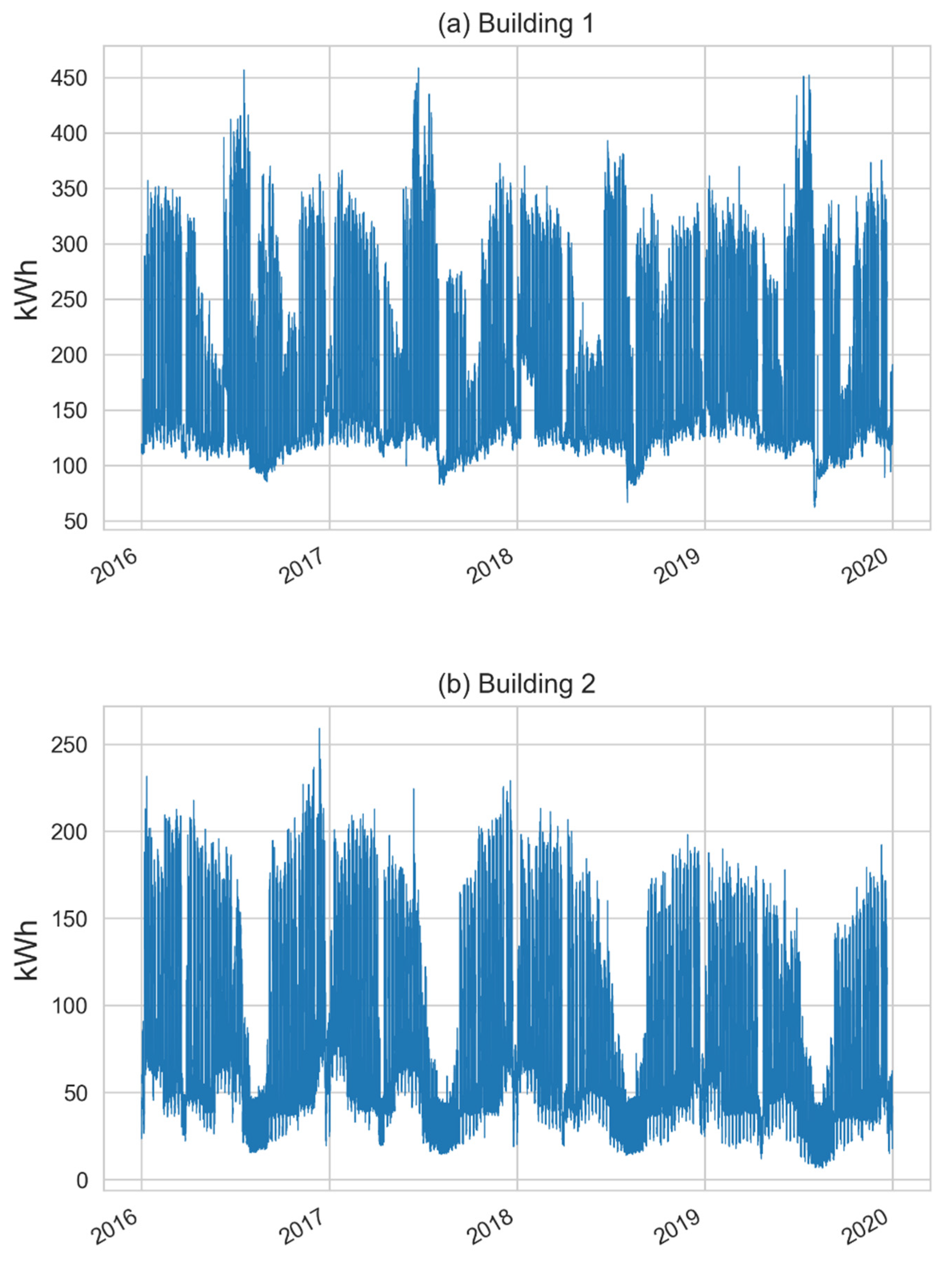
2.1. Data Collection

For this research, data from two buildings located on the campus of the University of Valladolid, Spain was used. The historical data of the energy consumption from 2016 to 2019 in 15 min intervals, was obtained through smart meters located in each of the buildings. Even though both buildings are located on a university campus, building 1 is more focused on administrative use where office areas are located in most of the building. In the case of building 2, the use is mixed, since there are classrooms, offices, and a library. Figure 1 shows the energy consumption and the overall pattern of each building throughout the timeframe analyzed.

The climatic data used for the construction of the dataset were obtained through NASA Prediction of Worldwide Energy Resources [19]. As the research is focused on sustainable buildings, variables that influence occupant comfort within buildings were considered. The following variables were considered for the training of the models: heating degree days below 18.3 °C (HDD18_3), cooling degree days above 0 °C (CDD0), cooling degree days above 10 °C (CDD10), precipitation (PRECTOT), relative humidity at 2 m (RH2M), the temperature at 2 m (T2M), the temperature at 2 m minimum (T2M_MIN), the temperature at 2 m maximum (T2M_MAX), and all-sky surface longwave downward irradiance (ALLSKY). An exploratory analysis of the data was made through a correlation heatmap to determine the relationship between the variable to be predicted (ENERGY) and the climatic variables, which is shown in Figure 2.

Figure 2 shows that there is a positive correlation with the variables HDD18_3, PRECTOT, RH2M and a negative correlation with the variables CDD0, CDD10, T2M, T2M_MIN, T2M_MAX, and ALLSKY. Similarly, it is observed that the correlations in both cases are weak. Therefore, it would be important to carry out another analysis to conclude which variables could contribute to the models.

In addition to the aforementioned data, the academic calendar of each year was obtained to use this information to determine the occupancy of the buildings considering the periods where occupancy is minimal.

Finally, an analysis to determine which values of the past series would be more useful to predict future values was carried out using autocorrelation function (ACF) and partial autocorrelation function (PACF).

Figure 3 shows the analysis performed for each building. It is observed in the autocorrelation graph that both datasets present patterns of seasonality, indicating that the use of autoregression models would be appropriate. In the partial autocorrelation graph, it is observed that until lag 25, there is significant autocorrelation in the time series, which would be important to consider for the models.

2.2. Data Preparation

To prepare the dataset that was used for the selected forecast models, the following steps were performed (see Figure 4):

• Data imputation. The raw data gathered for each building presented missing values. To solve this issue, the raw data were preprocessed. As the missing data were less than 0.3% of the total data, the linear interpolation method was used to solve the issue.
• Calendar data creation. To obtain a better result in the forecast, the following calendar variables were created: hour, weekday, month, and holiday.
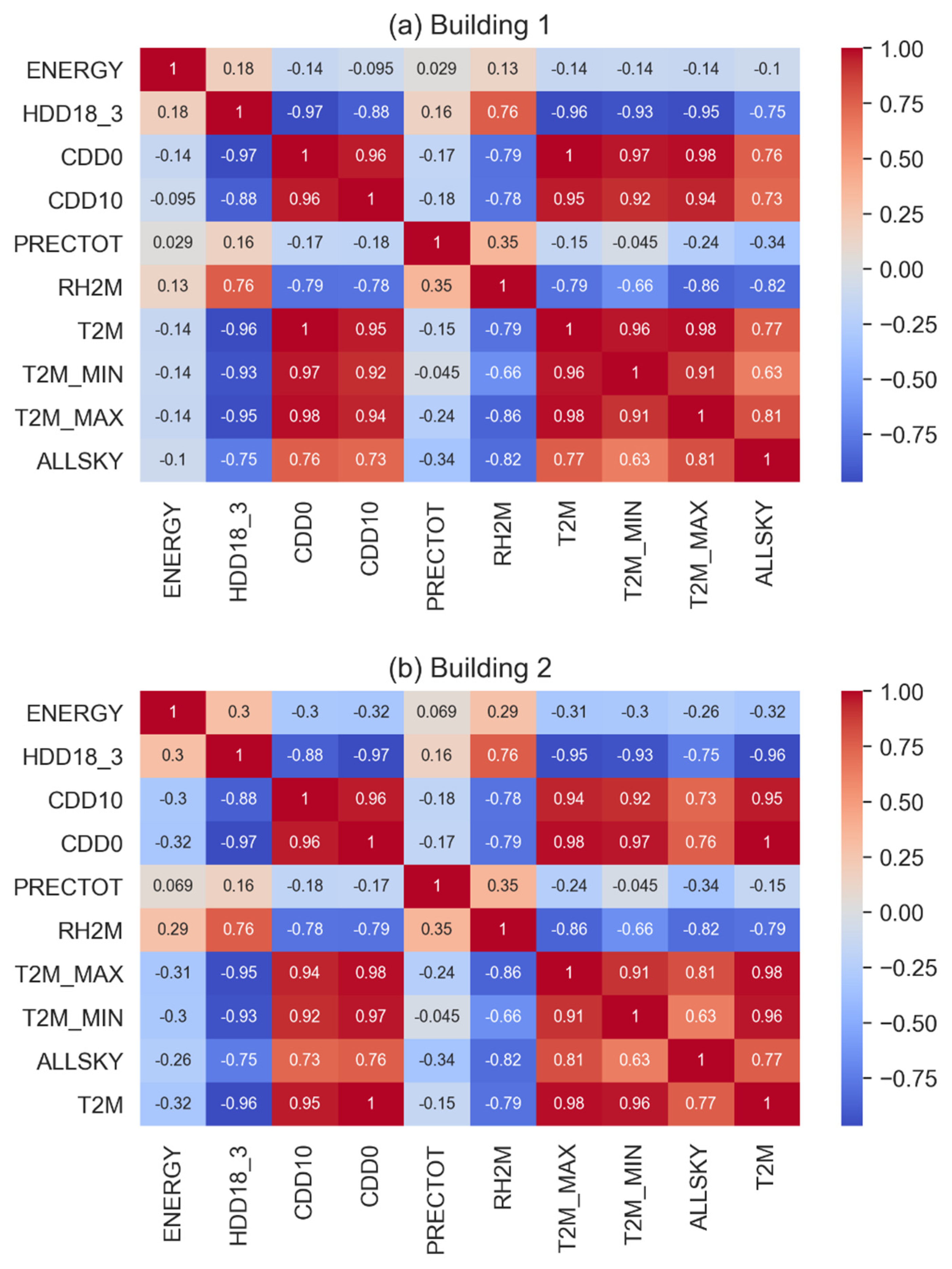
• Weather data preparation. To avoid adding error to the forecasting models by not knowing exactly the future values of the climatic variables, the values of the previous day were used.
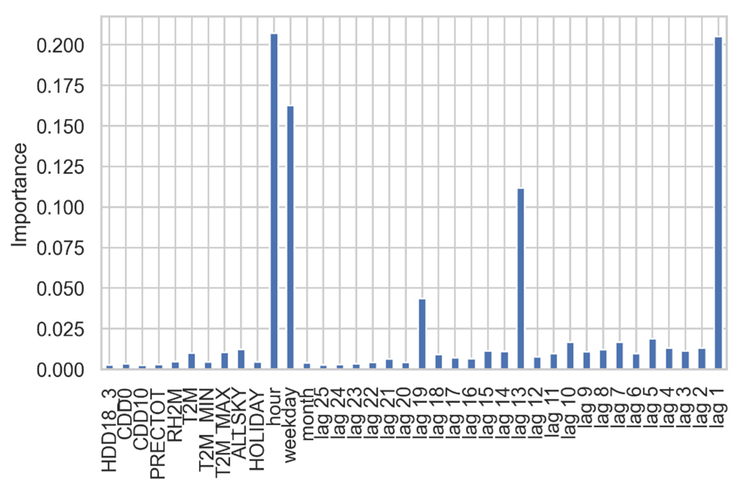
• Past series values creation. From the analysis of the ACF and PACF, the decision to use 25 time gaps was reached because after 25 lags the partial correlation decreases significantly.
• Dataset formation. After creating all the variables that would be used, the final dataset was built with the aforementioned steps.

3. Methodology and Approach

3.1. Selected Forecasting Models

For the selection of the models that were used to test the proposed strategy, the most popular data-driven models for forecasting demand [20,21,22,23,24,25] in buildings were considered. In addition to this, models that have not been as widely used as temporal convolutional network and temporal fusion transformer were included; the reason for this was to see if these models that have been promising in other areas could bring better results. A brief description of each one is presented below:

•

Multiple Linear Regression (MLR) is a statistical method generally utilized for time-series forecasting. The fundamental thought behind simple linear regression is to attempt to discover the connection between two variables. For the situation where various independent variables are utilized to decide the value of a dependent variable, the process is called multiple linear regression [26].

•

Artificial Neural Network (ANN) is planned to copy the fundamental architecture of the human brain, whose essential component is called a processing unit modeling a biological neuron. The network comprises a large number of these process units exhibited in layers, and process units in various layers are associated with each other via connections [27].

•

Random Forest (RF) is a model where a bunch of decision trees are utilized to create the last output, utilizing a democratic plan. Each tree is initiated from an arbitrarily chosen preparing subset and additionally utilizing a randomly chosen subset of highlights. This suggests that the trees rely upon the upsides of an autonomously tested information dataset, utilizing similar dispersion for all trees [28].

•

Extreme Gradient Boost (XGBoost): the fundamental thought behind this method is to adapt successively in which the current regression tree is fitted to the residuals from the past trees. This new regression tree is then added to the fitted model to refresh the residuals. The principle of gradient boosting further improves the adaptability of the boosting algorithm by developing the new regression trees to be maximally related to the negative of the gradient of the loss function [29].

•

Long-Term Short Memory (LTSM) comprises a memory block that is answerable for deciding the expansion and erasure of data through three entryways, namely input gate, forget gate, and output gate. The memory cell in the memory block recollects worldly state data about current and past timesteps [30].

•

Convolutional Neural Network(CNN) comprises of four fundamental parts: convolutional layer, which includes maps of the information; pooling layers, which are applied to lessen the dimensionality of the convoluted element; flattening, which changes the information into a column vector; and a connected hidden layer, which computes the loss function [31].

•

Temporal Convolutional Network (TCN) is a sort of convolutional neural network with a particular design that makes them appropriate for time series forecasting. TCN fulfills two primary standards: the network’s output has a similar length as the input arrangement, and they avoid leakage of data from the future to the past by utilizing causal convolutions [32].

•

Temporal Fusion Transformer(TFT) utilizes specific elements such as sequence-to-sequence and consideration-based temporal processing elements that catch time-fluctuating connections at various timescales; static covariate encoders that permit to condition temporal forecasts on static metadata; gating segments that empower skipping over unnecessary elements of the network; variable determination to pick important information at each time step, and quantile expectations to obtain output spans across all forecast horizons [33].

3.2. Forecasting Models Training, Tunning, and Execution

The dataset used to train and test the models was split into the years 2016 to 2018 for training and the year 2019 for testing. The models sought to forecast in a 24 h window, so in the training phase, the dataset was prepared to meet this requirement by using a strategy that would allow performing a forecast for each 24 h.

Before running the models for the 2019 forecast, the calibration of the models was performed which consisted of using the years 2016 and 2017 for training and 2018 for backtesting. This backtesting process was achieved by splitting the year 2018 into fivefold and testing a multi-step strategy using different hours to train the model. After performing this backtesting, the best parameters and architectures were used to train the final model.

During the model’s training phase, based on the correlation analysis of the climatic variables and the use of the mean decrease impurity (MDI) technique of the RF.

Figure 5 shows the results of the RF MDI technique, which was used to analyze which of the selected variables were significant for the models based on the score obtained. Several test runs were performed, which gave the results that the T2M, T2M_MAX, and ALLSKY variables were the ones that showed a slight improvement in the models during the backtesting. For this reason, we only decided to work with the climatic variables that contribute the most to the models.

For the tunning process, the following architectures, and individual hyper-parameters (see

Table 1. Forecasting models architectures and hyper-parameters.

Model	Python Library	Architectures and Hyper-Parameters
MLR	Scikit-learn	Does not have any hyper-parameters.
ANN	Scikit-learn	hidden_layer_sizes = (60, 30) learning_rate_init = 0.01 learning_rate = adaptive max_iter = 5000
RF	Scikit-learn	max_depth = 45 n_estimators = 200 min_samples_leaf = 1
XGBoost	Scikit-learnXGBoost	n_estimators = 200 eta = 0.1 max_depth = 5 colsample_bytree = 0.8 subsample = 0.8 gamma = 1
LSTM	TensorFlow	Two LSTM layers with 640 units and linear activation functions. batch size = 5 loss function = mean squared error. optimizer = adam learning rate = 0.0001 The model with the best epoch in the loss function was selected.
CNN	TensorFlow	Three convolutional hidden layers. First layer: 1D convolution with 512 filters, kernel size = 4, linear activation function, MaxPooling1D of size 2. Second layer: 1D convolution with 256 filters, kernel size = 4, linear activation function, MaxPooling1D of size 2. Third layer: 1D convolution with 256 filters, kernel size = 4, linear activation function. One fully connected layer with 200 units and linear activation function. Output layer with 24 units. loss function = mean squared error optimizer = adam learning rate = 0.001 batch size = 5 The model with the best epoch in the loss function was selected.
TCN	TensorFlow	filters = 400 kernel_size = 4 dilations = [1,2,4,8,16,32] batch size = 5 activation function = linear loss function = mean squared error optimizer = adam. learning rate = 0.0001. The model with the best epoch in the loss function was selected.
TFT	PyTorch	hidden_size = 700 lstm_layers = 2 attention_head_size = 4 drop rate = 0.21 batch_size = 128 hidden_continuous_size = 18 log interval = 10 learning rate = 0.0598 gradient_clip_value = 0.048 gradient_clip_val = 0.048 The loss function used was Quantile Loss with seven quantiles. The model with the best epoch in the loss function was selected. The calendar variables were used as time-varying known.

) were tested using different Python libraries:

The chosen values previously mentioned varying from the default values set by the separate libraries since they appeared to perform better. For models that were created with the scikit-learn library, grid search and randomized search [34] were used as parameter search techniques to obtain the best combinations of parameters. For other models, the best parameter combinations were obtained through backtesting. It should be noted that for models that do not natively support multi-target forecastings, such as MLR and XGBoost, a multi-output function was used which allowed this to be possible.

When the final model was already trained, the prediction of the year 2019 was made with each of the forecasting models and then evaluated by different accuracy metrics.

3.3. Accuracy Metrics

To evaluate the performance of the different models, accuracy metrics such as coefficient of determination (R²), root mean square error (RMSE), mean absolute error (MAE), and mean absolute percentage error (MAPE) were used.

R² analyzes how the model approximates the actual data and is calculated according to Equation (1) [35]:

$$R^2=1-\frac{{{\displaystyle \sum }}_{i=1}^n{\left(y_i-{ŷ}_i\right)}^2}{{{\displaystyle \sum }}_{i=1}^n{\left(y_i-{ŷ}_i\right)}^2}$$

(1)

RMSE analyze the precision of various anticipating standards and is calculated according to Equation (2) [36]:

$$RMSE=\sqrt{\frac{{{\displaystyle \sum }}_{i=1}^n{\left(y_i-{ŷ}_i\right)}^2}{n}}$$

(2)

MAE indicate the separation between anticipated and real value and is calculated according to Equation (3) [37]:

$$MAE=\frac{{{\displaystyle \sum }}_{i=1}^n\left|\frac{\left(y_i-{ŷ}_i\right)}{y_i}\right|}{n}$$

(3)

MAPE expresses average absolute error as a percentage and is calculated according to Equation (4) [38,39]:

$$MAPE=\frac{{{\displaystyle \sum }}_{i=1}^n\left|\frac{\left(y_i-{ŷ}_i\right)}{y_i}\right|}{n}\times 100\%$$

(4)

where $y_i$ is the anticipated value, ${ŷ}_i$ is the real value, ${ȳ}_i$ is the average value, and $n$ is the total number of estimates.

4. Results and Discussion

After evaluating the aforementioned models with the accuracy metrics, the results shown in

Table 2. Performance of each model by building.

	Building 1				Building 2
Model	R2	RMSE (kWh)	MAE (kWh)	MAPE (%)	R2	RMSE kWh)	MAE (kWh)	MAPE (%)
MLR	0.72	37.34	26.19	16.79	0.72	21.01	15.27	38.31
ANN	0.75	35.48	22.56	13.26	0.79	18.19	12.22	26.84
RF	0.83	29.45	16.2	9.22	0.86	15.16	9.15	19.68
XGBoost	0.85	27.23	15	8.83	0.87	14.12	8.22	17.92
LSTM	0.79	32.26	17.74	10.18	0.83	16.38	9.33	19.36
CNN	0.81	30.71	17.07	9.38	0.81	17.35	9.59	16.96
TCN	0.83	29.43	15.84	9.02	0.84	16.04	9.01	17.74
TFT	0.69	39.57	17.7	9.22	0.84	16.08	9.53	18.84

were obtained. Using the MAPE as a reference, it is observed that in building 1 the models that gave the best results were XGBoost, and TCN while in building 2 were CNN and TCN.

To improve the results obtained by the models with the proposed strategy, different tests were carried out. The tests consisted of combining the different models to obtain an assembled model (meanBest). The best combination was selected based on the lowest MAPE (see

Table 3. Performance of the assembled models.

	Building 1				Building 2
Assembled Model	R2	RMSE (kWh)	MAE (kWh)	MAPE (%)	R2	RMSE (kWh)	MAE (kWh)	MAPE (%)
C2	0.86	26.70	14.40	8.31	0.86	14.78	8.25	15.66
C3	0.86	26.73	14.43	8.27	0.88	13.81	7.69	15.44
C4	0.86	26.76	14.34	7.97	0.89	13.27	7.50	15.14
C5	0.86	26.42	14.20	7.85	0.89	13.31	7.48	15.31
C6	0.86	26.41	14.29	7.95	0.89	13.20	7.48	15.60
C7	0.86	26.43	14.62	8.17	0.89	13.28	7.69	16.40
C8	0.86	26.55	15.20	8.61	0.89	13.44	8.01	17.72

Cx = combination of x best models, x = number of models.

), which in this case was C5 for building 1 and C4 for building 2.

To validate that there is a significant difference between the models from the statistical point of view, an analysis of variance (ANOVA) for repeated measures and post hoc multiple pairwise comparisons between groups with Bonferroni correction, taken the MAPE as a measure of analysis was used between the best four simple models and the best-assembled model for each of the buildings; see

Table 4. ANOVA test results for building 1.

Model 1	Model 2	p-adj	Decision
meanBest	RF	1.97 × 10−171	True
meanBest	TCN	9.15 × 10−127	True
meanBest	TF	1.89 × 10−56	True
meanBest	XGB	5.09 × 10−102	True
RF	TCN	1.5 × 10−2	True
RF	TF	1	False
RF	XGB	5.03 × 10−14	True
TCN	TF	8.09 × 10−1	False
TCN	XGB	2.2 × 10−2	True
TF	XGB	7 × 10−3	True

p-adj = is the corrected p value using Bonferroni correction; decision = indicates if there is a significant difference.

for building 1 and

Table 5. ANOVA test results for building 2.

Model 1	Model 2	p-adj	Decision
CNN	meanBest	6.32 × 10−56	True
CNN	TCN	7.56 × 10−6	True
CNN	TF	8.53 × 10−51	True
CNN	XGB	3.89 × 10−11	True
meanBest	TCN	4.67 × 10−109	True
meanBest	TF	2.33 × 10−195	True
meanBest	XGB	5.99 × 10−254	True
TCN	TF	2.18 × 10−8	True
TCN	XGB	1	False
TF	XGB	1.89 × 10−9	True

p-adj = is the corrected p value using Bonferroni correction; decision = indicates if there is a significant difference.

for building 2.

The results of the ANOVA indicated that at least one MAPE is different, so multiple comparisons must be made to determine between which there are differences. According to Table 4 and Table 5, it can be mentioned that the MAPE of the meanBest is statistically different from the other models for both buildings.

However, when directly evaluating the RF and TF models, as well as the TCN and TF models, the test indicates that there is no significant difference between them for the case of building 1. The same case happens for the XGBoost and TCN models in building 2.

Figure 6 shows the behavior of both buildings concerning the days of the week, months of the year, and weeks of the year. When performing an analysis of the behavior of the models per day, it can be seen in a general way that the models maintain the same trend except for linear regression (LR) and neural network (NN). For LR, it is because it models linear relationships, which is clearly at a disadvantage before the other models that can capture non-linear relationships, while for the NN, it could not capture the non-linear relationships on specific days of the week.

As the week progresses, their margin of error decreases, with the days that show the greatest error in the prediction being Sundays and Mondays, due to opposite patterns when using past series values. The behavior by the week of the year presents a greater error from week 30 to week 32, this is because Holy Week does not occur on a particular date of the year, so the models have difficulty in adapting to this change. For the months of the year, it is observed that July and August are where the greatest error occurs since they coincide with the time of year where the university campus is not in its normal operation. Thinking that these events could affect the performance of the models, a variable was considered to measure when the university was in recess, however, the model generated a high error for these events.

Figure 7 shows the behavior of both buildings concerning the hours of the prediction and the period of prediction. The hours of prediction correspond to the performance of the proposed strategy with each of the models in each hour of the day, emphasizing that for both buildings the interval between 10 a.m. and 12 p.m. is where the best results are obtained. The period of prediction corresponds to the performance of the strategy as the hours go by, showing that the first hours are the ones that present the least error in the forecast.

Figure 8 shows the actual forecast of the assembled model that obtained the best result for each hour of the forecasted year, which in the case of building 1 was the combination of the best five models, while for building 2, it was the combination of the best four models.

5. Conclusions

Machine learning and deep learning models are important techniques for building energy forecasting, so it is necessary to accompany them with strategies that can make the most of these techniques. In this paper, an energy consumption forecasting strategy to predict day-ahead hourly energy consumption in smart buildings is presented and tested on real data from two buildings located in Valladolid, Spain. The proposed strategy is different from other strategies because it can predict the energy consumption of the next 24 h at any hour of the day, which is of interest to smart buildings and microgrids.

For the energy consumption forecast, a dataset composed of historical data, meteorological data, calendar data, and past series values was used. Different machine learning and deep learning models were used to test the strategy. Of those models, the best ones were considered for the build of an assembled model using the mean of the prediction values. In general, the assembled models obtained better results than the single models. The assembled model with the combination of five models was the best one for building 1 with a MAPE of 7.85% and the assembled model with the combination of four models was the best one for building 2 with a MAPE of 15.14%. Confirming what authors such as [40,41] have mentioned that the combination of several forecasting models can cancel out random errors, achieving in some cases more accurate forecasts.

We are currently working to improve the accuracy of the prediction. In the same way, future lines of research would be to improve the composition of the dataset including occupancy data to achieve better adaptability of the forecast when there are radical changes such as the periods when the university closes and when it starts, which is where it has been seen that the model generates the greatest error. As well as being able to reduce the learning patterns of the strategy to make it possible to use it with fewer patterns and obtain better results.

References

1. Deb, C.; Zhang, F.; Yang, J.; Lee, S.E.; Shah, K.W. A Review on Time Series Forecasting Techniques for Building Energy Consumption. Renew. Sustain. Energy Rev. 2017, 74, 902–924. [Google Scholar] [CrossRef]
2. Somu, N.; MR, G.R.; Ramamritham, K. A Deep Learning Framework for Building Energy Consumption Forecast. Renew. Sustain. Energy Rev. 2021, 137, 110591. [Google Scholar] [CrossRef]
3. Zhang, C.; Li, J.; Zhao, Y.; Li, T.; Chen, Q.; Zhang, X. A Hybrid Deep Learning-Based Method for Short-Term Building Energy Load Prediction Combined with an Interpretation Process. Energy Build. 2020, 225, 110301. [Google Scholar] [CrossRef]
4. Son, N.; Yang, S.; Na, J. Deep Neural Network and Long Short-Term Memory for Electric Power Load Forecasting. Appl. Sci. 2020, 10, 6489. [Google Scholar] [CrossRef]
5. Runge, J.; Zmeureanu, R. A Review of Deep Learning Techniques for Forecasting Energy Use in Buildings. Energies 2021, 14, 608. [Google Scholar] [CrossRef]
6. Jordan, M.I.; Mitchell, T.M. Machine Learning: Trends, Perspectives, and Prospects. Science 2015, 349, 255–260. [Google Scholar] [CrossRef] [PubMed]
7. Zhang, L.; Wen, J.; Li, Y.; Chen, J.; Ye, Y.; Fu, Y.; Livingood, W. A Review of Machine Learning in Building Load Prediction. Appl. Energy 2021, 285, 116452. [Google Scholar] [CrossRef]
8. Fan, C.; Sun, Y.; Xiao, F.; Ma, J.; Lee, D.; Wang, J.; Tseng, Y.C. Statistical Investigations of Transfer Learning-Based Methodology for Short-Term Building Energy Predictions. Appl. Energy 2020, 262, 114499. [Google Scholar] [CrossRef]
9. Fang, X.; Gong, G.; Li, G.; Chun, L.; Li, W.; Peng, P. A Hybrid Deep Transfer Learning Strategy for Short Term Cross-Building Energy Prediction. Energy 2021, 215, 119208. [Google Scholar] [CrossRef]
10. Ding, Y.; Zhang, Q.; Yuan, T. Research on Short-Term and Ultra-Short-Term Cooling Load Prediction Models for Office Buildings. Energy Build. 2017, 154, 254–267. [Google Scholar] [CrossRef]
11. Lopez-Martin, M.; Sanchez-Esguevillas, A.; Hernandez-Callejo, L.; Arribas, J.I.; Carro, B. Novel Data-Driven Models Applied to Short-Term Electric Load Forecasting. Appl. Sci. 2021, 11, 5708. [Google Scholar] [CrossRef]
12. Moon, J.; Jung, S.; Rew, J.; Rho, S.; Hwang, E. Combination of Short-Term Load Forecasting Models Based on a Stacking Ensemble Approach. Energy Build. 2020, 216, 109921. [Google Scholar] [CrossRef]
13. Somu, N.; MR, G.R.; Ramamritham, K. A Hybrid Model for Building Energy Consumption Forecasting Using Long Short Term Memory Networks. Appl. Energy 2020, 261, 114131. [Google Scholar] [CrossRef]
14. Yang; Tan; Santamouris; Lee Building Energy Consumption Raw Data Forecasting Using Data Cleaning and Deep Recurrent Neural Networks. Buildings 2019, 9, 204. [CrossRef] [Green Version]
15. Ishaq, M.; Kwon, S. Short-Term Energy Forecasting Framework Using an Ensemble Deep Learning Approach. IEEE Access 2021, 9, 94262–94271. [Google Scholar] [CrossRef]
16. Xue, P.; Jiang, Y.; Zhou, Z.; Chen, X.; Fang, X.; Liu, J. Multi-Step Ahead Forecasting of Heat Load in District Heating Systems Using Machine Learning Algorithms. Energy 2019, 188, 116085. [Google Scholar] [CrossRef]
17. Kolokas, N.; Ioannidis, D.; Tzovaras, D. Multi-Step Energy Demand and Generation Forecasting with Confidence Used for Specification-Free Aggregate Demand Optimization. Energies 2021, 14, 3162. [Google Scholar] [CrossRef]
18. Shao, X.; Kim, C.S. Multi-Step Short-Term Power Consumption Forecasting Using Multi-Channel LSTM with Time Location Considering Customer Behavior. IEEE Access 2020, 8, 125263–125273. [Google Scholar] [CrossRef]
19. NASA POWER NASA Prediction of Worldwide Energy Resources. Available online: https://power.larc.nasa.gov/ (accessed on 1 February 2021).
20. Mariano-Hernández, D.; Hernández-Callejo, L.; García, F.S.; Duque-Perez, O.; Zorita-Lamadrid, A.L. A Review of Energy Consumption Forecasting in Smart Buildings: Methods, Input Variables, Forecasting Horizon and Metrics. Appl. Sci. 2020, 10, 8323. [Google Scholar] [CrossRef]
21. Peng, L.; Wang, L.; Xia, D.; Gao, Q. Effective Energy Consumption Forecasting Using Empirical Wavelet Transform and Long Short-Term Memory. Energy 2021, 121756. [Google Scholar] [CrossRef]
22. Bourhnane, S.; Abid, M.R.; Lghoul, R.; Zine-Dine, K.; Elkamoun, N.; Benhaddou, D. Machine Learning for Energy Consumption Prediction and Scheduling in Smart Buildings. SN Appl. Sci. 2020, 2, 297. [Google Scholar] [CrossRef] [Green Version]
23. Kathirgamanathan, A.; De Rosa, M.; Mangina, E.; Finn, D.P. Data-Driven Predictive Control for Unlocking Building Energy Flexibility: A Review. Renew. Sustain. Energy Rev. 2021, 135, 110120. [Google Scholar] [CrossRef]
24. Bendaoud, N.M.M.; Farah, N. Using Deep Learning for Short-Term Load Forecasting. Neural Comput. Appl. 2020, 32, 15029–15041. [Google Scholar] [CrossRef]
25. Lu, H.; Cheng, F.; Ma, X.; Hu, G. Short-Term Prediction of Building Energy Consumption Employing an Improved Extreme Gradient Boosting Model: A Case Study of an Intake Tower. Energy 2020, 203, 117756. [Google Scholar] [CrossRef]
26. Divina, F.; García Torres, M.; Goméz Vela, F.A.; Vázquez Noguera, J.L. A Comparative Study of Time Series Forecasting Methods for Short Term Electric Energy Consumption Prediction in Smart Buildings. Energies 2019, 12, 1934. [Google Scholar] [CrossRef] [Green Version]
27. Wei, Y.; Zhang, X.; Shi, Y.; Xia, L.; Pan, S.; Wu, J.; Han, M.; Zhao, X. A Review of Data-Driven Approaches for Prediction and Classification of Building Energy Consumption. Renew. Sustain. Energy Rev. 2018, 82, 1027–1047. [Google Scholar] [CrossRef]
28. Breiman, L. Random Forests. Mach. Learn. 2001, 45, 5–32. [Google Scholar] [CrossRef] [Green Version]
29. Chakraborty, D.; Elzarka, H. Early Detection of Faults in HVAC Systems Using an XGBoost Model with a Dynamic Threshold. Energy Build. 2019, 185, 326–344. [Google Scholar] [CrossRef]
30. Luo, X.J.; Oyedele, L.O.; Ajayi, A.O.; Akinade, O.O.; Owolabi, H.A.; Ahmed, A. Feature Extraction and Genetic Algorithm Enhanced Adaptive Deep Neural Network for Energy Consumption Prediction in Buildings. Renew. Sustain. Energy Rev. 2020, 131, 109980. [Google Scholar] [CrossRef]
31. Goodfellow, I.; Bengio, Y.; Courville, A. Deep Learning; MIT Press: Cambridge, MA, USA, 2016; ISBN 0262035618. [Google Scholar]
32. Lara-Benítez, P.; Carranza-García, M.; Luna-Romera, J.M.; Riquelme, J.C. Temporal Convolutional Networks Applied to Energy-Related Time Series Forecasting. Appl. Sci. 2020, 10, 2322. [Google Scholar] [CrossRef] [Green Version]
33. Lim, B.; Arık, S.Ö.; Loeff, N.; Pfister, T. Temporal Fusion Transformers for Interpretable Multi-Horizon Time Series Forecasting. Int. J. Forecast. 2021, in press. [Google Scholar] [CrossRef]
34. Pedregosa, F.; Varoquaux, G.; Gramfort, A.; Michel, V.; Thirion, B.; Grisel, O.; Blondel, M.; Prettenhofer, P.; Weiss, R.; Dubourg, V.; et al. Scikit-Learn: Machine Learning in Python. J. Mach. Learn. Res. 2011, 12, 2825–2830. [Google Scholar]
35. Amasyali, K.; El-Gohary, N.M. A Review of Data-Driven Building Energy Consumption Prediction Studies. Renew. Sustain. Energy Rev. 2018, 81, 1192–1205. [Google Scholar] [CrossRef]
36. Ali, U.; Shamsi, M.H.; Bohacek, M.; Hoare, C.; Purcell, K.; Mangina, E.; O’Donnell, J. A Data-Driven Approach to Optimize Urban Scale Energy Retrofit Decisions for Residential Buildings. Appl. Energy 2020, 267, 114861. [Google Scholar] [CrossRef]
37. Khosravani, H.; Castilla, M.; Berenguel, M.; Ruano, A.; Ferreira, P. A Comparison of Energy Consumption Prediction Models Based on Neural Networks of a Bioclimatic Building. Energies 2016, 9, 57. [Google Scholar] [CrossRef] [Green Version]
38. Xu, X.; Meng, Z. A Hybrid Transfer Learning Model for Short-Term Electric Load Forecasting. Electr. Eng. 2020, 102, 1371–1381. [Google Scholar] [CrossRef]
39. Hu, H.; Wang, L.; Lv, S.-X. Forecasting Energy Consumption and Wind Power Generation Using Deep Echo State Network. Renew. Energy 2020, 154, 598–613. [Google Scholar] [CrossRef]
40. Chan, F.; Pauwels, L.L. Some Theoretical Results on Forecast Combinations. Int. J. Forecast. 2018, 34, 64–74. [Google Scholar] [CrossRef]
41. Makridakis, S.; Spiliotis, E.; Assimakopoulos, V. The M4 Competition: 100,000 Time Series and 61 Forecasting Methods. Int. J. Forecast. 2020, 36, 54–74. [Google Scholar] [CrossRef]
Figure 1. (a) Energy consumption and general trends of building 1; (b) energy consumption and general trends of building 2.
Applsci 11 07886 g001
Figure 2. (a) Correlation heatmap between climatic variables for building 1; (b) correlation heatmap between climatic variables for building 2.
Applsci 11 07886 g002
Figure 3. (a) ACF and PACF graphs for the time series of building 1; (b) ACF and PACF graphs for the time series of building 2.
Applsci 11 07886 g003
Figure 4. Data preparation steps for dataset formation.
Applsci 11 07886 g004
Figure 5. Random forest feature importance.
Applsci 11 07886 g005
Figure 6. (a) Performance of forecasting models by day, month, and week in building 1; (b) performance of forecasting models by day, month, and week in building 2.
Applsci 11 07886 g006
Figure 7. (a) Performance of forecasting models by the hour, and prediction period in building 1; (b) performance of forecasting models by the hour, and prediction period in building 2.
Applsci 11 07886 g007
Figure 8. (a) Real versus predicted energy consumption for building 1; (b) real vs. predicted energy consumption for building 2.
Applsci 11 07886 g008