Convolutional Neural Networks for Automated Rolling Bearing Diagnostics in Induction Motors Based on Electromagnetic Signals

Abstract

Bearing faults account for over 40% of induction motor faults, and for this reason, for several decades, much attention has been paid to their condition monitoring, through vibration measurements and, more recently, through electromagnetic signal analysis. Furthermore, in the last few years, research has been focused on evaluating deep learning algorithms for the automatic diagnosis of these faults. Therefore, the purpose of this study is to propose a novel procedure to automatically diagnose different types of bearing faults and load anomalies by means of the stator current and the external stray flux measured on the induction motor in which the bearings are installed. All the data were collected by performing experimental tests in the laboratory. Then, these data were processed to obtain images (scalograms and spectrograms), which were elaborated by a pre-trained Deep Convolutional Neural Network, modified through the transfer learning technique. The results demonstrated the ability of the electromagnetic signals, and in particular of the stray flux, to detect bearing faults and mechanical anomalies, in agreement with the recent literature. Moreover, the Convolutional Neural Network has been proven to be able to automatically discriminate bearing defects and with respect to the healthy condition.

1. Introduction

Rolling bearings are purely mechanical elements; nevertheless, they represent a critical factor for the safe operation of rotating electrical machines. In fact, if their maintenance is disregarded, i.e., if they are not correctly lubricated and/or substituted in due time, they can fail, causing the breakdown of the electrical machine. Moreover, a harsh environment with pollutants, humidity, and high temperature can accelerate bearing wear. Last but not least, the power supply of electrical motors by means of electronic converters can arouse shaft voltage and bearing currents if the bearing is not properly insulated, with a consequent early fault of the bearing itself [1].

For these reasons, and considering that bearing faults represent more than 40% of induction motor faults [2,3], for the last several decades, much attention has been focused on the condition monitoring of rolling bearings, initially based on vibration measurements and more recently on the measurement of electromagnetic signals coming from the electrical machine in which they are installed, i.e., stator current and external stray flux.

Bearing diagnostics through vibration analysis is mainly based on the evaluation of harmonics at specific frequencies, depending on which surface of the bearing contains the fault (outer race, inner race, rolling element, cage), on the geometrical dimensions of the bearing, and on the rotational speed of the rotor [3]. This technique is effective if the fault is localized (single-point), while in the case of generalized roughness, i.e., when the fault is spread over the entire bearing, other algorithms, like envelope analysis, have to be applied for processing the collected vibrations [4]. Vibration measurements require the installation of additional sensors, such as accelerometers, while current and stray flux measurements can take advantage of the sensors already present in the electrical drive to control of the motor.

For this reason, since 1995 [5], many studies have investigated the potential of analyzing the current as an alternative diagnostic signal for bearing fault detection and, since 2006 [6], the external stray flux has also been considered for the same purpose. The research group of this paper has previously investigated the advantages offered by electromagnetic signal analysis for bearing diagnostics, in particular, Motor Current Signature Analysis (MCSA) for single-point defects and generalized roughness [7], stray flux analysis for single-point defects [8], and both signals for identifying different steps of generalized roughness [9]. More recently, electromagnetic signals proved to be efficient in detecting bearing defects and other mechanical faults. In particular, in [10], two fault severities in the rolling elements and cage of a bearing were recognized via MCSA in an induction motor of 5.5 kW, while in [11], an inner race fault was identified by means of vibration, current, and stray flux analysis in an induction motor of 4 kW. From the comparative study presented in [11], the stray flux seems to provide the best results, as it is insensitive to external vibrations of the motor; nevertheless, the authors suggest using this signal in combination with at least one of the other signals, to increase the reliability of the diagnosis. In [12], the ability of MCSA and stray flux analysis has been evaluated in detecting mechanical faults in industrial cases, concerning induction motors of several hundred kilowatts, supplied at 6 kV; the experimental results of this research revealed that: (i) MCSA is highly sensitive to mechanical faults and is superior to vibration analysis, as well as having low cost and remote monitoring capabilities; (ii) stray flux is insensitive to the mechanical oscillations coming from the load but is more sensitive to the rotor eccentricity and misalignment than MCSA; (iii) stray flux seems unable to detect bearing faults of the entire system consisting of motor, shaft, and pump; (iv) one signal alone (vibration, current, or stray flux) seems unable to provide a comprehensive screening of the electrical machine. Therefore, the authors suggest combining at least two methods among vibration, current, and stray flux analysis. It is worth to noting that the outcomes presented in [12], although very interesting and well supported by experimental measurements in the field, are related to high power motors, and the flux sensors have been installed on the case of the machines, quite distant to the position of the bearings. Hence, it is likely that this type of installation makes it difficult to collect the stray flux containing information about the health of the bearings. It is also important to observe that, in all the papers cited so far, the diagnostic approach was based on the evaluation of the amplitude of specific harmonics of the faults in the spectra of the vibrations or electromagnetic signals; this approach is typical of condition monitoring of the electrical machines, which is complementary to fault diagnosis.

In fact, fault diagnostics have been developed by means of these two main approaches: (i) condition monitoring, which is related to the first two stages of diagnostics, i.e., data acquisition and processing; (ii) fault diagnosis, which concerns the last stage, i.e., decision making.

Condition monitoring research is aimed at studying the ability of different sensors and processing techniques to identify characteristic signatures in mechanical and electromagnetic signals, which represent the characteristics of specific failures. These characteristics are generally related to the machine parameters (e.g., type of machine, number of poles, number of rotor and stator slots, bearing geometry, etc.) and its working conditions (e.g., speed, load percentage, type of power supply, etc.). Therefore, a deep knowledge of the machine is necessary, not only to identify these signatures, but also to choose the threshold which separates the faulty condition from the healthy condition of the machine, which can heavily influence the probability of committing an error during the decision-making phase. This decision can be made by an individual or by an automatic algorithm.

Fault diagnosis research is mainly focused on algorithms able to automatically discriminate the presence of a fault, on the basis of signals coming from the monitored machine. These techniques can be classified in Machine Learning (ML) and Deep Learning (DL); ML techniques include Artificial Neural Network (ANN), Principal Component Analysis, and other methods, which have been known for at least three decades, while DL algorithms have been developed in the last five years [13]. Both ML and DL algorithms require a wide collection of data to be trained, such as datasets available online [14] or extensive laboratory measurement campaigns [15,16]. But while ML methods rely on human-engineered features in the training process, DL algorithms prove automated feature extraction capabilities and better classification performance [17].

With respect to traditional ANNs, in the branch of the DL, the main difference of the network architectures is that they have more than one hidden layer. A network designed with this criteria, i.e., the Deep Neural Network (DNN), can give outstanding classification accuracy if trained with enough data. Besides the classification accuracy, other favorable characteristics of this kind of network are the automatic feature extraction during the training process and greater ease to adapt the network to other purposes, with the transfer learning technique [17]. In the DL context, Convolutional Neural Networks (CNNs) gained popularity because of their shared weights topology which allows them to delve deeper, thereby achieving very good classification accuracy, with fewer parameters required for training than a fully connected topology [18].

A very thorough and detailed review on DL for bearing fault diagnostics was published last year [17]; therefore, the analysis of the state-of-the-art research presented here will be limited to a few recent papers. In [19], the publicly available dataset of the Case Western Reserve University (CWRU) [20] was used to train a DNN. In this case, the time-domain signals were transformed into the frequency domain and features were extracted from the spectra to reduce the high data dimension to a small dimension before entering the data into the DNN for training; in this way, the dataset was not based on an expert or previous knowledge, as in traditional ANN. In [21], the CNN AlexNet was modified by only replacing the last fully connected layer; the raw acceleration signals were converted into uniformly sized time-frequency images, even when the data had different sizes. The proposed method was tested on both experimental measurements carried out in the laboratory and CWRU dataset. In [22], a transfer learning CNN based on AlexNet was proposed for bearing fault diagnosis, wherein a 2D image representation method converts vibration signals to 2D time-frequency images. Then, the proposed CNN model extracts the features of the 2D time-frequency images and achieves the classification conditions of the bearing, which is faster to train and more accurate. The bearing data from CWRU was used to verify the performance of the proposed method. The work presented in [23] is particularly interesting because it tested the validity of a CNN on both test bench data and actual service data, measured on a locomotive running on the real line. The faults considered were in the inner ring, outer ring, and roller of a bearing. In [24], a CNN model based on the AlexNet was proposed to classify the wear level of bearings, by using a dataset from the center of Intelligent Maintenance Systems. Even the authors of the present paper have already considered two pre-trained networks for diagnostic purposes [25]. Other recent works have investigated further variants of these networks, named “Deep Residual”, and tested them on measurements from experimental test benches in the laboratory [26,27].

It is evident that fault diagnostics of electrical machines implies the acquisition of several measurements from the machine and a post-elaboration of the data for diagnosis purposes. To this end, the use of automatic DL methods is becoming more and more useful and effective. In particular, CNNs are usually applied with the aim of classification of faults. In order to have good accuracy, a CNN should be well trained, with a lot of different samples, measured from different machines and in various operating conditions. This is obviously not always possible, due to the dangers that arise from running a faulty machine and the high number of different operating conditions (speeds and load) [17]. An approach which showed good accuracy while allowing for a small number of samples is based on pre-trained networks [21,22,24].

Other works use the transfer learning technique for bearing diagnosis, such as with a 1D-CNN taken from a ResNet model in [28] and with a GoogLeNet model and 2D signal transformation in [29]. However, both papers only considered vibration and not electromagnetic signals.

Based on all the above considerations, this paper proposes a novel procedure to automatically diagnose different types of bearing faults and load anomalies by means of electromagnetic signals coming from the induction motor in which the bearings are installed. The data are converted into 2D representations through the use of Continuous Wavelet Transforms and Short-Time Fourier Transforms. There are at least a two original aspects of this work: the use of data collected by performing experimental tests in the laboratory and the development of a neural metamodel based on CNN for processing electromagnetic signals from the machine being tested. To the authors’ knowledge, although many papers use the current signal analysis with Wavelet Transforms for bearing diagnosis (some references are reported in Section 2), as of yet, no one has dealt with bearing fault diagnosis by means of Wavelet Transforms and ML models of machines’ stray flux signals. Moreover, in this work, a double fault condition was investigated: the simultaneous presence of torque oscillation and a bearing fault. In addition, two different types of bearing fault that are difficult to treat together were considered: the generalized roughness and the single-point defect.

Paper Structure

Stray flux and current measurements were used in this work, performed on an induction motor. The measurements were done in both the conditions of healthy motor and different bearing faults. The bearing faults considered were the following: two types of generalized roughness (“step 1” and “step 2” roughness, as described below) and a single-point defect in the outer ring in four different positions.

Moreover, in order to test our method in a more difficult condition, the Low Frequency Torque Oscillation (LFTO) was added in some cases (double fault condition). The experimental setup is described in Section 3.

The measured signals were processed with time-frequency transformations; for the sake of a comparison, either the Continuous Wavelet Transform (CWT) or the Short Time Fourier Transform (STFT) were used. In particular, the CWT generated the so-called “scalograms”, while the STFT generated classical “spectrograms”. The methods used for the time-frequency transformations are detailed in Section 2.1.

In order to estimate the effect of a different sampling frequency of the measurements on the fault detection capability, the time-frequency transformation with both the CWT and STFT was also performed for the so-called “decimated data”, i.e., data with a lower acquisition frequency.

The images obtained (scalograms or spectrograms, decimated or non-decimated) were elaborated by a Deep Convolutional Neural Network, GoogLeNet [30].

The CNN GoogLeNet is trained in this work for classification purposes by means of the transfer learning technique. In fact, GoogLeNet is a pretrained net; the use of a pretrained net is necessary when the number of samples for training the net is small, as it was in this case. The CNN approach used in the paper is presented in Section 2.2.

Multi-class classification of faults was considered in this work, namely:

• three classes (healthy, generalized roughness step 1, generalized roughness step 2) in Section 4.1;
• three classes (as before) and decimated data in Section 4.1.1;
• seven classes (three classes as in Section 4.1 and four classes relevant to a localized crack in the outer ring in four different angular positions) in Section 4.2; in particular, only flux measurements, only current measurements, and both kinds of measurements were investigated in Section 4.2.1, Section 4.2.2 and Section 4.2.3, respectively; moreover, in Section 4.2.3, a comparison between decimated and non-decimated data is shown;
• four classes (relevant to a localized crack in the outer ring in four different angular positions) with and without the presence of the LFTO in Section 4.3.1;
• eight classes and LFTO (four classes relevant to a localized crack in the outer ring in four different angular positions and four classes for the same faults but with the LFTO added) in Section 4.3.2.

All the previous cases were implemented with GoogLeNet fed by scalograms.

In Section 4.4.1 and Section 4.4.2, the same classes as those used in Section 4.3.1 and Section 4.3.2 were considered, but the SFTF (spectrograms) was used instead of the CWT (scalograms) for the time-frequency transformation. Moreover, decimated data were considered. Finally, Section 5 and Section 6 report a final discussion and the conclusion of the overall work.

2. Materials and Methods

In this work, time-frequency domain images obtained from signals measured on an induction motor with bearings with different types of faults were used as input for a CNN. In particular, the signals from the current sensor and the radial external stray flux sensor of an induction motor were transformed into the time-frequency domain via the Continuous Wavelet Transform (CWT), which generates scalograms; for comparison, transformations with the Short Time Fourier Transform (STFT), which produces graphs called spectrograms, are also presented.

The choice to use the wavelet transform arose from the fact that many papers have recently used it for the diagnostics of electrical machines, such as in [31]. Regarding bearing defects in particular, interesting findings can be found in [32,33], where a Discrete Wavelet Transform (DWT) and a CWT were used on vibration signals for the diagnosis of bearing defects. In [34], a wavelet packet decomposition and a Hilbert envelope were used on the motor current signal for bearing fault detection. Other works dealing with Wavelet Transforms for the diagnosis of induction machines include [35,36,37]. Lastly, in [38], an analysis of the motor current signal through a CWT is presented. To the knowledge of the authors of this paper, there are currently no publications available demonstrating wavelet analysis of machines’ stray flux for bearing fault recognition.

The signals analyzed came from an induction motor fed by an inverter, which implies more difficulties in the classification of the faults as stated in various works throughout the literature, such as in [39,40]. One of the prevailing difficulties lies in the fact that the frequency of the current waveform could be variable for the speed control of the machine, and this can lead to transients in which the characteristic harmonics of the sought faults cannot be correctly identified with a normal frequency-domain analysis. Another important difficulty is that the electronic commutations carried out in the inverter for the generation of the waveform determine the formation of Electromagnetic Interference (EMI), which could easily cover the characteristic fault harmonics. The last main difficulty in searching for faults in electronic-fed drives is the presence of a closed-loop control, especially used in Field Oriented Control (FOC) drives. In fact, as stated in [41], while it could still be possible to see fault harmonics with an open loop V/f controlled driver, with a FOC closed-loop it is not possible to diagnose bearing faults via normal current and voltage measurements (without any change on the FOC structure). Many techniques have been implemented in various works to reduce these effects on the diagnostic system, especially for the detection of bearing faults that have very low characteristic harmonic amplitudes, for incipient faults in particular.

It is often stated in the literature that the analysis of vibration signals could be the best choice for the diagnosis of the bearings, because the bearings’ mechanical faults generate a change in the signature of the vibrations as a primary effect. The harmonics in the current or stray flux spectra come from secondary effects of the fault, i.e., change in the air-gap distribution (air-gap eccentricity) and introduction of torque ripples due to the fault in the bearing [5,42]. Besides this, vibration measurements could be difficult in some cases because the machine could not be easily accessible and the costs of purchase and maintenance of the sensors could be high and increase the complexity of the system. Moreover, the vibration signature could change from one physical point of the machine to another; for example, it could be necessary to install more than one accelerometer to check both the fan-end and drive-end bearings.

Although current signal is often considered to be not sufficient for the complete diagnosis of the bearing and should be combined with the vibration signal [42], many works try to extrapolate diagnosis information only from this signal because of the ease of installation of the sensor or the cheapness of using a sensor already installed for the inverter control.

In this work, both current and external stray flux signals were used for the monitoring of the machine. The stray flux analysis proved to be as effective as the current signature analysis and in some cases can give better diagnostic results [43]. In this contribution, as already mentioned, the analysis of the current and radial stray flux signals was carried out by means of a CNN, through the transfer learning technique, for the purpose of classification of the healthy and faulty signals.

2.1. Time-Frequency Transformation: Scalograms and Spectrograms

A spectrogram is a visual representation of the spectrum frequencies of a signal as it varies with time. A spectrogram can be generated in various ways. In this work, the STFT and CWT were used to generate spectrograms. In particular, with the wavelet transform, the images generated are also known as scalograms. In this work, the nomenclature “spectrograms” refer to the STFT images only, while “scalograms” refer to the CWT images.

One way to create a spectrogram from a time-domain signal is to approximate it through the use of a filterbank that results from a series of band-pass filters; otherwise, it is possible to do it through the repetitive use of the Fast Fourier Transform (FFT) algorithm. In this second approach, which is much more widespread in digital signal processing, the digitally sampled data in the time-domain are subdivided into windows, which usually overlap each other, and then Fourier transformed to calculate the frequency spectrum of each window. Every window spectrum then corresponds to a vertical line in the image in which the color intensity is proportional to the relative magnitude of the signal at the considered frequency. These line spectra are then laid “side by side” or slightly overlapped with windowing functions to form the complete spectrogram image.

With the STFT, the main limitation is that the resolution is fixed. The width of the retrieved windows determines whether there is a good frequency resolution, in which two near harmonics can be distinguished on the spectra, or a good time resolution, with which one can see the rapid changes in time of the frequency components. This is summarized by the Gabor limit, which states that a signal cannot be simultaneously sharply localized in the time and frequency domain with the STFT.

In the continuous-time case of the short-time Fourier transform, the function to be transformed is multiplied by a function which is always zero except for a short time-period (a window function). The Fourier transform of the signal is composed as the window shifts along the time axis, resulting in a two-dimensional representation of the signal [44]:

$$STFT\left\{x\left(t\right)\right\}\left(\tau ,\omega \right)\equiv X\left(\tau ,\omega \right)={{\displaystyle \int }}_{-\infty }^{\infty }x\left(t\right)\omega \left(t-\tau \right)e^{-i\omega t}dt$$

(1)

where $\omega \left(\tau \right)$ is the window function (it could be a Hann window or Gaussian window function) and $x\left(t\right)$ is the signal to be transformed.

In discrete time transformations, the data to be transformed is subdivided into time-frames which usually overlap to reduce the artifacts. Each frame is Fourier transformed and the magnitude and phase of the complex value for each point in time and frequency is stored:

$$STFT\left\{x\left[n\right]\right\}\left(m,\omega \right)\equiv X\left(m,\omega \right)={\displaystyle \sum }_{n=-\infty }^{\infty }x\left[n\right]\omega \left(n-m\right)e^{-i\omega n}$$

(2)

where $x\left[n\right]$ is the signal and $\omega \left(n-m\right)$ is the window, with $m$ and $\omega$ being discrete and continuous values, respectively. However, in practical use, both variables are discrete.

Finally, the Power Spectral Density (PSD) is a function that describes the power present in the signal as a function of frequency, per unit frequency.

The squared magnitude of the STFT yields the spectrogram representation of the Power Spectral Density of the function:

$$spectrogram\left\{x\left(t\right)\right\}\left(\tau ,\omega \right)\equiv {\left|X\left(\tau ,\omega \right)\right|}^2$$

(3)

In contrast to the STFT, a wavelet transform is made through the convolution operation of a signal with functions called wavelets. A wavelet is a wave-like oscillation with an amplitude that starts and ends at the zero value. A wavelet could be created to have a particular frequency; if this wavelet is convolved with a signal, then the resulting signal would be useful to determine whether the particular frequency was present in the signal. Sets of complementary wavelets are generally needed to fully analyze the data.

The wavelet analysis, in contrast to the STFT, presents a windowing technique with windows of variable size. This permits the use of long time intervals where more precise low-frequency information is required, and shorter windows where high-frequency information is required. The wavelet analysis is then not only more appropriate for the analysis of transient signals but also for reducing noise in the process.

In this work, a CWT was used. The CWT, unlike the DWT, lets the translation and scale parameters of the wavelets vary continuously, providing a complete representation of the signal. The scale parameter is the equivalent of the period parameter (the inverse of the frequency) in a periodic signal; it can stretch or shrink the wavelet with respect to its value. A shrunk scale can individuate slow changes in the signal while a stretched one localizes rapid transients in the analyzed signal.

In mathematics, the CWT is a tool that gives a complete representation of a signal with the translation and scale parameter of the wavelets, which vary continuously. The CWT of a function $x\left(t\right)$ at a scale $\left(a>0\right)$ with $a\in {ℝ}^{+*}$ and a translational value $b\in ℝ$ is expressed by the integral [45]

$$X_{\omega }\left(a,b\right)=\frac{1}{{\left|a\right|}^{1/2}}\underset{-\infty }{\overset{\infty }{{\displaystyle \int }}}x\left(t\right)\overline{\psi } \left(\frac{t-b}{a}\right)dt$$

(4)

where $\psi \left(t\right)$ is a continuous complex function in both the time and frequency domains (the so-called “mother wavelet”); the $\psi \left(t\right)$ function in (4) is complex conjugated (denoted by the overline symbol). The principal purpose of the mother wavelet is to give a source function to generate the daughter wavelets, which are simply the translated and scaled versions of the mother wavelet.

In this work, the CWT was processed through a filterbank in which 12 voices per octave were used; this means that there were 12 intermediate scale values for each octave. This discretization of the scale is not very high but it was considered to be suitable for the acceptable classification results achieved by the network. The wavelet used in the filter bank is the analytic Morse (3,60). This wavelet has a gamma value (symmetric parameter) of 3, which means it is symmetric in the frequency domain. The wavelet has a time-bandwidth product of 60. This parameter cannot exceed 40 times the gamma value; a higher value corresponds to greater spread of the wavelet in the time domain but also to a better frequency resolution.

The length of the input signal windows and the sampling frequencies used have been varied for the specific cases analyzed and are reported in the following sections.

More details on scalogram generation are presented in Section 4.1, where the first results are shown, although the same parameters are used in all the sections where a CWT was performed. Correspondingly, more details on the generation of spectrograms are reported in Section 4.4.

2.2. CNN Approach

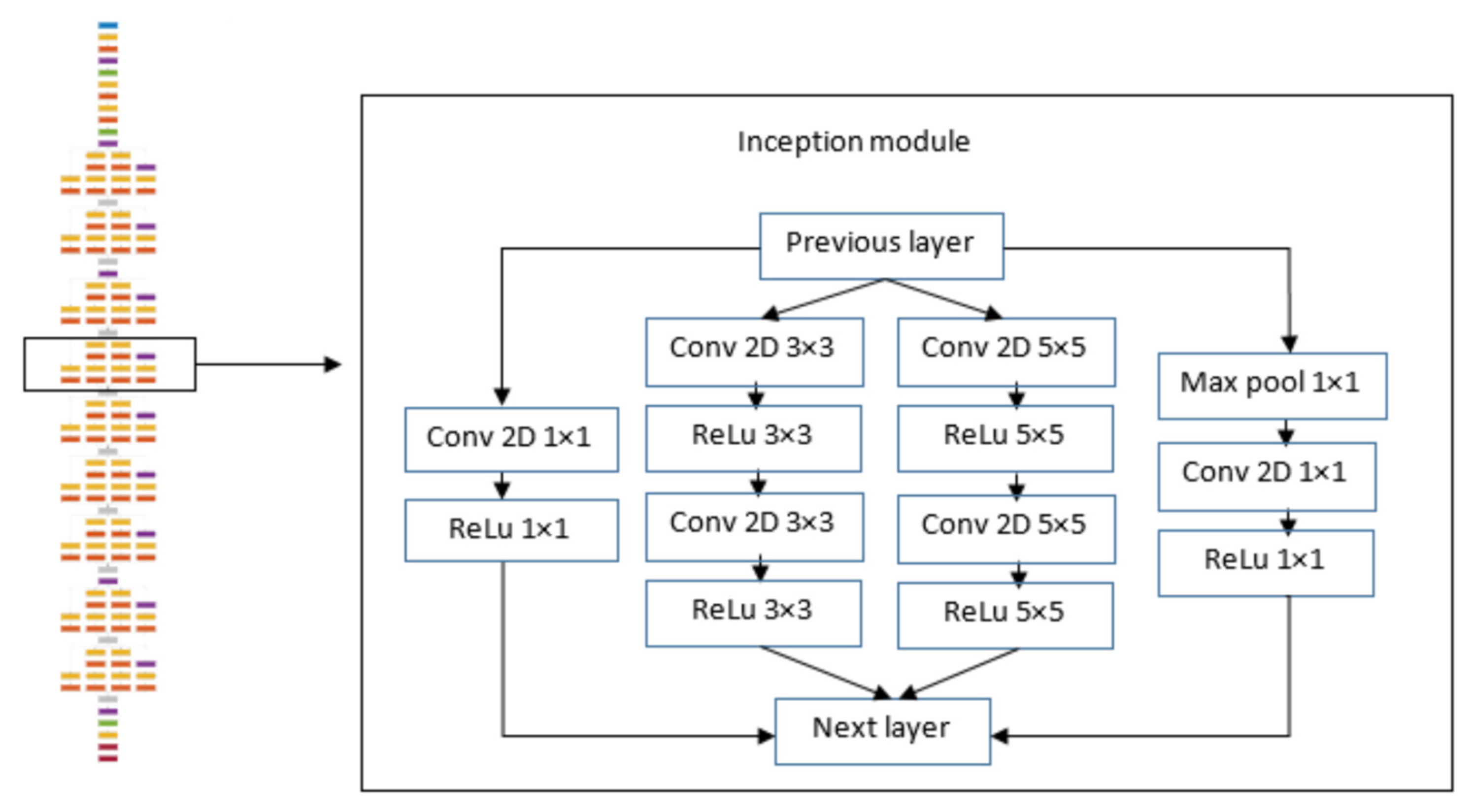
The convolutional neural network used in the paper, GoogLeNet, is a variant of the Inception Network, a Deep Convolutional Neural Network developed by researchers at Google. It is characterized by 22 layers, and part of these layers are included in a total of nine inception modules. Inception modules are usually used in CNNs for a more efficient computation and deeper networks, through a dimensionality reduction. The modules were designed to solve the problem of computational expense, as well as overfitting, among other issues. The solution, in short, is to take multiple kernel filter sizes within the CNN, and rather than stacking them sequentially, ordering them to operate on the same level. With this type of adaptation, it can be said that the network becomes wider rather than deeper. The net structure used in this paper is shown in Figure 1, with the scheme of the inception module highlighted.

As stated in the original research paper of the inventors of GoogLeNet [46], the inception modules are introduced with three different convolution filter sizes: 1 × 1, 3 × 3, and 5 × 5. Moreover, a max pooling is used in parallel, since it should improve the network performance as stated in the current literature. The parallel paths of the inception block give a feature extraction with various scales (the sizes of the filters), which are then aggregated before being retrieved by the next stage, so that it can abstract features from different scales simultaneously. The use of many convolution stages and inception blocks would result in an abnormal number of parameters to train if no dimensionality reduction method was used. So the main method used is a 1 × 1 convolution filter interposed before each of the computationally more expensive 3 × 3 or 5 × 5 filters of the parallel paths in the inception blocks.

An example of the specific network used in this work, available from the MATLAB repositories in its entirety, can be found in [47]. The dimensionality reduction blocks are marked with the suffix “_reduce”. To have a comparable dimension of the vectors leaving the pooling blocks, the 1 × 1 convolution filters are also used to project this output to the next concatenation block. They are marked with the “_proj” suffix.

An inception network is a network composed of inception modules stacked upon each other, with occasional intermediate max-pooling layers to reduce the resolution of the grid. However, as stated in [46], it might be convenient to begin the sequence of inception modules after some initial classic old-style convolutional layers. In this work, the pre-trained network was modified by replacing some of the final layers, as will be explained below.

The GoogLeNet version used in this paper was pre-trained on the ImageNet dataset [48]. This dataset is composed of 1000 different categories of images, such as objects and animals. The input of the net was a 224 × 224 pixel image, with three Red Green Blue (RGB) channels.

Although many works in the literature use 1D CNN with raw bearing vibration data [49,50], the choice of a 2D CNN was made to have a wider availability of pre-trained at state-of-progress networks used in image recognition. Moreover, with a 2D representation, even transient signals can be successfully studied, as shown in [51]. The choice of GoogLeNet, instead of using other networks such as VGG (Visual Geometry Group) or ResNet, was made for the good accuracy achieved by GoogLeNet in relation to its memory usage and computational resources required.

In the tests presented, the network was fed with diagnostic images of the machine, which are the scalograms and spectrograms as described in the previous section. These images are not part of the original classes the network was initially trained with, so in order to have an accurate classification process, the network had to be adapted. This was done by means of the transfer learning technique; this technique essentially consists of replacing the final fully-connected and classification layer with new ones with a number of output classes equal to the number of the classes of the new task (which must be at least one or two orders of magnitude less than the number of the original classes). The replaced layers are the fully-connected “loss3-classifier” and the “output” layer. The “prob” layer is a softmax classification probability layer and automatically adjusts the number of inputs, so it did not need to be replaced.

After the replacement of these final layers, the network required much less data to be retrained, as the first layers were already trained and correctly extracted the features from the images (in the particular case of a 2D CNN). Large learning rate factors (weight and bias learning rates) were used to allow the final layer to learn quickly, while small learning rate factors were kept for the initial layers because these layers do not have to change their learning parameters. This technique is useful because it eliminates the need for a complete design and training from scratch of a new network built for this purpose.

An additional modification on the network besides the replacement of the final fully-connected and classification layers was the modification of the final dropout layer (“pool5-drop_7 × 7_s1”). A dropout layer is a layer which randomly sets the input elements to zero to prevent the overfitting phenomenon; in the network used, the final dropout layer, located just before the final fully-connected layer, was modified, changing its dropout probability from 50% to 60%.

The particular adapted network used had a number of output classes set to the number of faults to detect (from three to eight faults). The training set was composed of 65% of the database images, the validation set was composed of 25% of the images, while the test set was composed of the remaining 10%. The images for creating the training, validation, and test datasets were chosen randomly. These sets were used for the direct training of the network, for the tuning of the hyper-parameters, and for the testing of the network (presented with the confusion matrices).

The net was trained with the Stochastic Gradient Descent with Momentum (SGDM) method for tens of epochs depending on the specific test. The minibatch size, i.e., the number of images used in each iteration, was set to six samples, and the initial learning rate was set to 10⁻⁴. The cross entropy function was chosen as the loss function of the SGDM optimizer. The specific parameters used for the specific tests are presented in Section 4. The goodness of the net was evaluated by means of both the validation accuracy and the confusion matrix, this last performed only with the test set.

3. Experimental Setup

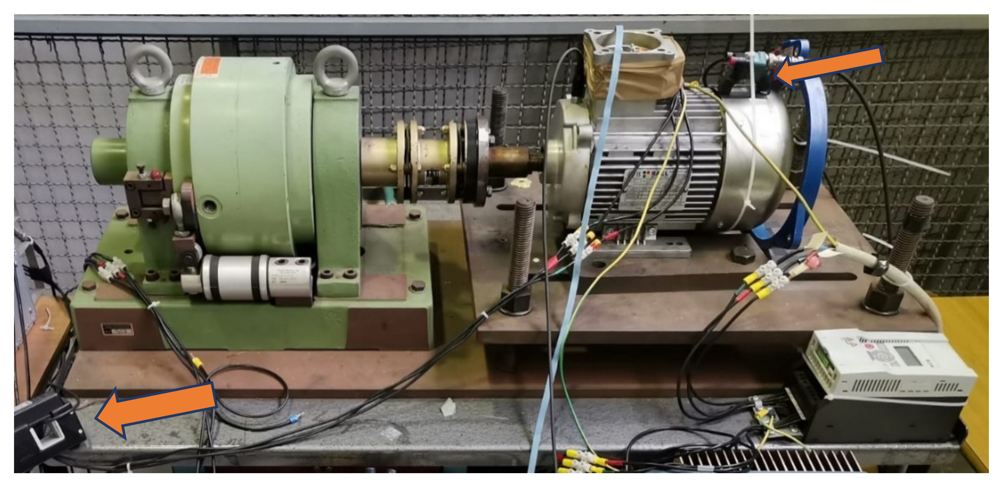
All the measurements presented in this paper come from experimental laboratory tests. The experimental setup used is the same as in the previous publications of the authors, such as in [52]. The test bed consisted of an explosion proof squirrel cage induction motor of 1.5 kW, wye-connected, coupled to a magnetic-powder brake through an elastic joint. The induction motor was fed by means of a 2.2 kW open loop Space Vector PWM (Pulse Width Modulation) inverter, model MMX34AA5D6F0-0 from the brand Moeller.

The brake can be easily modulated to obtain variable load torques through a variation of its excitation current. In fact, some tests reported in this paper used an oscillating load torque: a low frequency sinusoidal torque was added to a constant average load torque to obtain the Low Frequency Torque Oscillation (LFTO) condition. This situation can simulate some types of load, e.g., reciprocating compressors, where torque depends on the angular shaft position. The LFTO could also simulate a broken rotor bar defect; in fact, as a consequence of the asymmetry in the air-gap flux distribution due to the broken bar, an oscillating electromagnetic torque is produced. The torque oscillation generates sidebands around the fundamental supply frequency given at the frequency

$$f_{sb\_osc}=f_s\pm k·f_{osc}$$

(5)

While for the case of the broken rotor bars, the sidebands will be at frequency

$$f_{brb}=f_s\pm 2·k·s f_s$$

(6)

where f_s is the supply frequency, f_osc is the frequency of the torque oscillations, and k is an integer (usually considered as k = 1, 2, 3).

In addition to the power components, the experimental setup was composed of the following sensors: a current sensor based on a Hall effect, two stray flux sensors (one for the axial flux and one for the radial flux), and two accelerometers. The test bed is shown in Figure 2.

In this paper, only measurements from the radial stray flux sensor and from the current sensor are analyzed. The stray flux sensor was composed of a C-shaped ferrite nucleus, on which 300 turns of 0.112 mm diameter wire were wound. The sensor was located on the final part of the body of the motor, with its longitudinal axis parallel to the axis of the motor. As stated in a previous work [53], this position has been recognized to be the most effective for the diagnosis of the motor, at least for the detection of stator partial short circuits. The current sensor used was a Hall-effect sensor from the brand Tektronix, model TCP305 (Beaverton, OR, USA). The characteristics of the current sensor are shown in

Table 1. Features of the Tektronix TCP (Transmission Control Protocol) 305 current sensor.

Features	Values
Bandwidth	0–50 MHz
Current-carrying capacities	25 A DC
	17.7 A rms
	50 A peak
Typical precision	1% of the measured value
Sensibility	5 mA

.

The data were sampled from the various sensors with a multichannel NI-USB6212 Data Acquisition Board. The chosen sampling frequency was 120 kHz, due to the fact that the switching frequency of the inverter is 6 kHz and, following the procedure already used in [54], to correctly evaluate the harmonic distortion introduced by the inverter, a sampling frequency of 20 times the switching frequency was considered to be more adequate.

For antialiasing purposes, a hardware single-order low-pass filter was introduced into the measurement chain, between each sensor and the DAQ board. The bandwidth frequency selected for the filter was approximately 2 kHz.

The experimental tests were carried out with two types of bearings and two different faulty conditions of the bearing: generalized roughness (bearing wear) and a single-point defect (specifically a crack) on the outer ring of the bearing. This second condition was evaluated for different angular positions of the crack, similarly to the measurements reported in [20]; in fact, the weight of the rotor affects the intensity of the faulty signals, as reported in [55], so a crack located exactly under the direction of the weight should generate higher vibrations and displacements of the rotor in the air-gap. The bearing used for the simulations of the two types of fault were different. Their main characteristics are reported in

Table 2. Main characteristics of the bearings used.

Bearing Model	Fault Simulated	Number of Balls	Ball Diameters
NSK 6205Z	Single-point defect	9 (single row)	d ≅ 7.9 mm
SKF 1205ETN9	Generalized roughness	26 (double row)	d = 7.45 mm

.

The single-point defect on the outer ring of the bearing gives rise to characteristic harmonics on the vibration spectra expressed by:

$$f_o=BPFO=N/2·f_r\left(1-d/D·cos\alpha \right)$$

(7)

where BPFO stands for Ball Pass Frequency Outer, referring to a fault in the outer ring; N is the number of bearing balls; $f_r$ is the motor rotational frequency in hertz, d and D are the ball and pitch diameters, respectively; and α is the ball contact angle.

In the electromagnetic signals, the characteristic harmonics are visible as sidebands of the supply frequency:

$$f_p=\left|f_s\pm k{f}_o\right|$$

(8)

where k is a positive integer and $f_o$ is calculated from (7).

Regarding the generalized roughness, it does not manifest harmonics at specific frequencies, but the spectra of vibration and stator current of the machine change in an unpredictable way, often giving rise to broadband harmonic excitation [56].

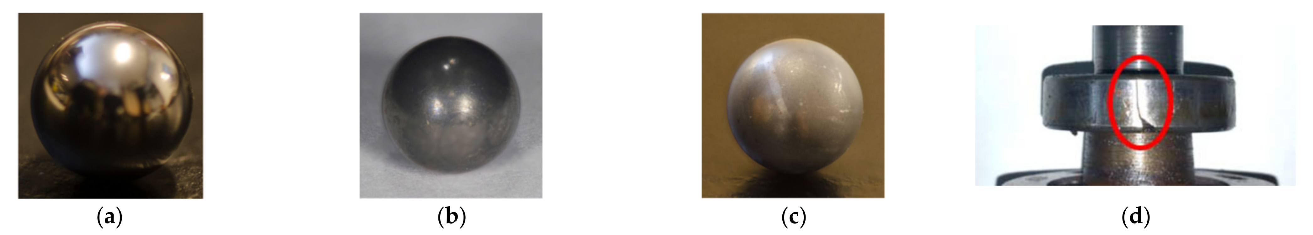
For the tests with generalized roughness, two fault severity levels were used in addition to the healthy measurements, considered as the baseline; Step 1 and Step 2 faults were generated through the use of acid corrosion wear as described below. Step 1 represents an early stage; the bearing was disassembled and all balls were degreased and immersed for 30 min in a solution composed of 5 mL of concentrated sulfuric acid (96%) dissolved in 50 mL of water. Step 2 represents an advanced stage; all balls were immersed for 70 min in a solution identical to that of Step 1. A representation of the balls worn by the acid solution and the localized fault is reported in Figure 3.

The single-point defects consisted of a localized crack in the outer ring of the bearing in four different angular positions; the angular position of the defect was marked as an hourly index, as shown in Figure 4. The analyzed fault locations were at hours 12, 3, 4.5, and 6, and in the following, they will be denoted by H12, H3, H45, and H6, respectively.

The acquisition parameters for each case are shown in

Table 3. Characteristics of each set of acquisitions.

N° of Sample for Each Acquisition	Acquisition Frequency	Achievable FFT Resolution	Number of Acquisitions	Time of the Whole Set
220 = 1,048,576	120 kHz	0.115 Hz	40	40 × 8.73 = 349 s

. Each case analyzed was composed of several acquisitions to obtain measurements distributed over a longer time period for the purpose of thermal stability and for calculating the mean of the spectra to reduce noise as in previous works, such as in [52,54]. The exact number of the acquisitions could change from 40 to 80 for each class depending on the particular test carried out. The number of images are presented in the following section, in

Table 4. Denotation and number of images generated for each faulty condition (in the Denotation column, BF means Bearing Fault).

Type of Fault	Denotation	Number of Images Generated
Baseline	Bas	80
Generalized roughness step 1	BF Step 1	40
Generalized roughness step 2	BF Step 2	40
Crack at hour 12	H12	60
Crack at hour 3	H3	60
Crack at hour 4.5	H45	60
Crack at hour 6	H6	60

.

In this paper, a generalized roughness bearing defect and a single-point defect in the outer ring were investigated. During this research, no data were available relating to other types of bearing defect (e.g., inner ring defect, ball defect, etc.) and compatible with those analyzed by the authors. Although only two types of defects that could happen in a bearing were investigated, the authors believe that if the network can discriminate between two different hour-case single-point defects in the outer ring, then there could be a very similar signature between them, and it could also discriminate other different types of defect.

4. Results

This work, as already established, presents a data analysis through the use of a pre-trained neural network of signals from an induction motor with defective bearings and bearings in healthy condition. In this section, the various tests conducted with the modified deep neural network GoogLeNet are presented. The signals of stator current and radial stray flux have been converted via various techniques and then analyzed via the transfer learning technique.

For the transformation of the raw data into the time-frequency domain, different cases were considered: (i) the use of CWT versus STFT techniques, (ii) the use of decimated versus non-decimated data, and (iii) the use of only one sensor signal versus the use of two signals. In addition, the low frequency torque oscillation condition signal (only for the current signal) was introduced for testing the proposed CNN approach in a more challenging scenario. All the elaborations were computed in a MATLAB environment, with the use of the deep learning toolbox and the wavelet toolbox. The computer used for the elaborations was an ASUS (Taipei, Taiwan) laptop of medium characteristics model “VivoBook S15 X530FN”, with dedicated NVIDIA “GEFORCE MX150” GPU and 16 Gb of RAM. All the computations were elaborated on the GPU through the MATLAB parallel computing toolbox.

4.1. Tests with Three Classification Classes

The first tests were conducted with only three classification classes: healthy (baseline), faulty with generalized roughness Step 1, and faulty with generalized roughness Step 2.

The number of images was 80 for the baseline and 40 for each of the cases Step 1 and Step 2. The transformation used was the CWT with a filter bank; the sampling frequency imposed was 120 kHz and the voices per octave were 12. The MATLAB function used to create the filter bank was “cwtfilterbank”. By default, the filters are normalized so that the peak magnitudes for all passbands are approximately equal to 2. The highest frequency passband is designed so that the amplitude falls to half the peak value at the Nyquist frequency. For the objective of this work, where several similar signals were analyzed in time-frequency, the filter bank was precomputed at the beginning and then passed as input for the “wt” function that returns the coefficients of the CWT.

As implemented, the CWT uses L1 normalization. With L1 normalization, equal amplitude oscillatory components at different scales have equal magnitude in the CWT. Moreover, L1 normalization gives a more accurate representation of the signal. The magnitudes of the oscillatory components agree with the magnitudes of the corresponding wavelet coefficients.

With a real value signal, “wt” returns a 2D matrix of coefficients, in which each row corresponds to one scale, while the columns represent the time instants and every column has the same length as the signal considered. The final matrices from which the scalogram images were derived were obtained by computing the absolute value of the wavelet coefficients.

To convert from indexed images (the coefficient matrices) to RGB images, the “ind2rgb” function was used (it outputs the three RGB channels with pixel values in the range 0–1). The chosen color map was “jet”, with 128 colors. Every image was generated with the “imwrite” function and had a size of 224 × 224 pixels. To ensure that the generated scalogram had this exact size in order to be fed to the input layer of the network, the “imresize” function was used. By default, this function uses the bicubic interpolation, where the output pixel value is a weighted average of the pixels in the nearest 4-by-4 neighborhood.

The images were generated using the first 100,000 samples of each acquisition. With a sampling frequency of 120 kHz, this resulted in an interval of 833 ms. This time interval was considered to be long enough, as it contained approximately 41 fundamental cycles (all the tests were carried out with a 50 Hz fundamental frequency imposed by the inverter). In the cases in which more than 40 images were generated for each class, in addition to the first 100,000 sample segments of each acquisition, other consecutive segments of 100,000 samples were taken from the same 2²⁰ sample acquisitions.

Moreover, a data augmentation was used to increase the number of images in the training dataset, whereby a random reflection over the x-axis was executed and a random translation on the x and y axis of max 30 pixels was also carried out. The hyper-parameter set for the modified GoogLeNet had a “minibatch size” of 6 and a maximum number of epochs of 9. The other modifications made to accommodate the transfer learning technique are described in Section 2.2.

The weight and bias learning rate factor for the final fully connected layer of the substituted network was chosen to be equal to 15. This means that the new substituted layer learnt 15 times faster than the transferred layers.

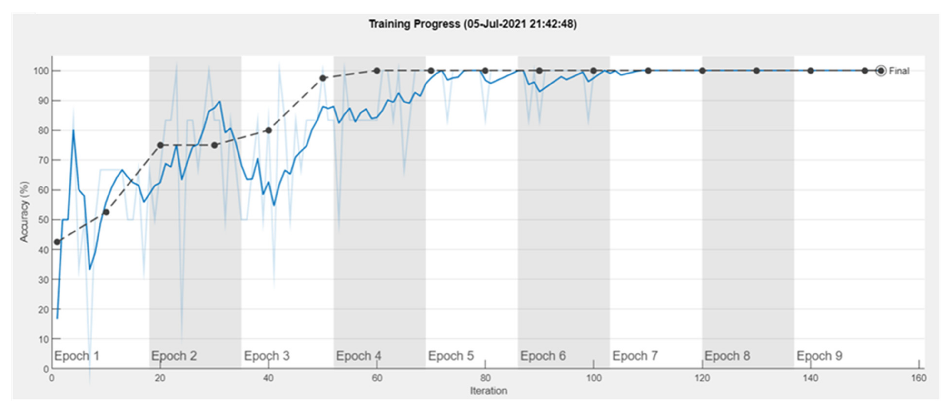
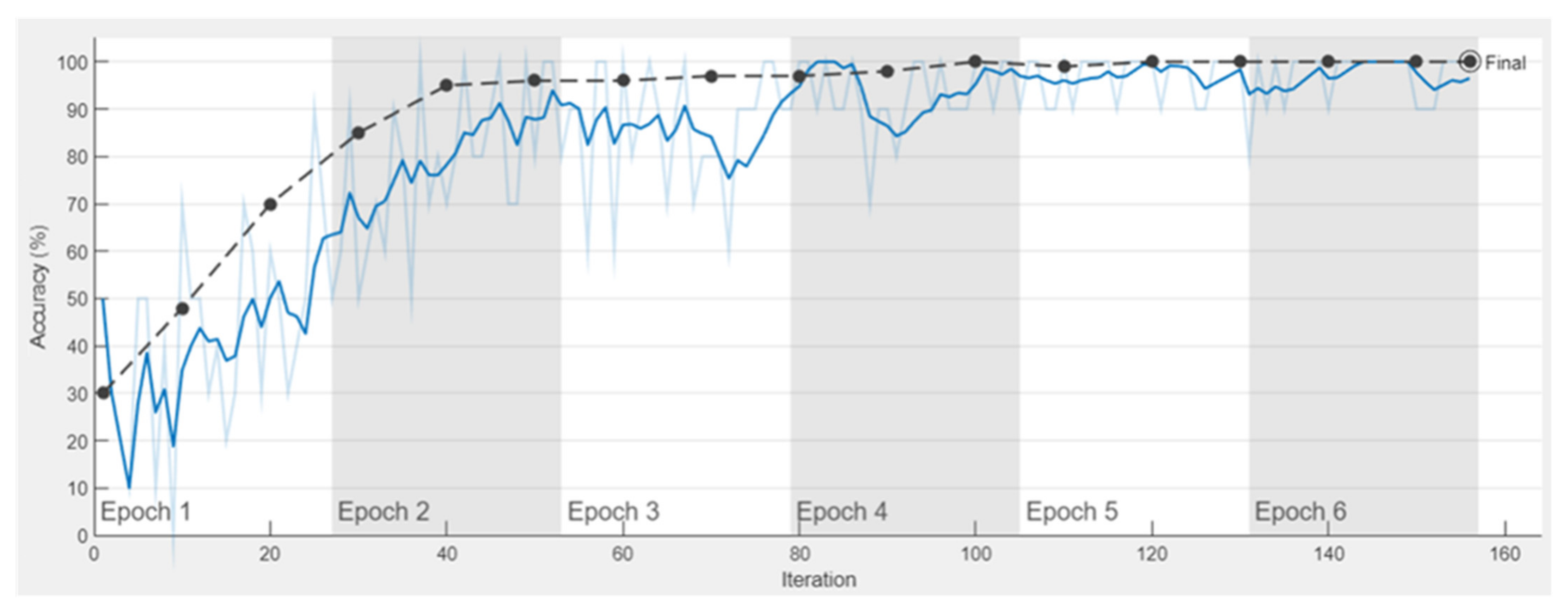
Some random images for the radial stray flux and current signal are shown in Figure 5. The validation accuracies reached with the network fed with the two signals are 100% and 50% for the radial flux and current signal, respectively. An example of the training progress is shown in Figure 6. As can be seen from Figure 6, the network reached convergence quite quickly (after 4 epochs) and the full process lasted less than a minute. The confusion matrices for the two cases are shown in Figure 7.

The test accuracy for the flux signal (93.8%) was a little less than the validation accuracy, while the test accuracy for the current signal (50%) was the same as the validation accuracy.

From these first tests, it is clear that the radial flux signal gives better results than the current signal with the same transformation parameters.

4.1.1. Tests with Three Classification Classes and Decimated Data

The same tests carried out with the full sampling frequency were repeated with a sampling frequency decimated. These tests were carried out because the sampling frequency usually assumes lower values and the fault characteristic patterns searched are at lower frequencies, i.e., ranging from 0 to 2 kHz.

For the decimation of the sampling frequency, the “decimate” MATLAB function was used. This function includes a lowpass Chebyshev Type I infinite impulse response (IIR) filter of order 8 for the purpose of antialiasing.

The reduction factor chosen was 10, so the new sampled frequency was then 12 kHz and the signal length was 10,000 samples.

For the sake of a comparison, a decimated sampling image obtained from the current signal and a non-decimated one are shown in Figure 8.

The validation accuracies obtained with these decimated data were 97.5% and 40.0% for the radial flux and current signals, respectively. This means that the images could also be recognized with a decimated sampling frequency, although with a decrease in the validation accuracy for both flux and current signals (from 100% to 97.5% for the radial flux and from 50% to 40% for the current).

4.2. Tests with Seven Classification Classes

Further tests were carried out by adding four classes related to bearings with a localized crack in the outer ring in four different angular positions. The data were processed in the same way as described previously in Section 4.1 and fed to the network, which had the same hyper-parameters imposed. The data used were non-decimated. The name of the classes with the number of images generated in each class are shown in Table 4.

4.2.1. Analysis of the Radial Stray Flux Signal

With the radial stray flux, the accuracy of the network also remained very high with seven classification classes. The network reached convergence quickly, as can be seen in Figure 9; it reached convergence in about 4 epochs, with a validation accuracy of 100%. The confusion matrix is reported in Figure 10, showing that every class was recognized correctly.

4.2.2. Analysis of the Current Signal

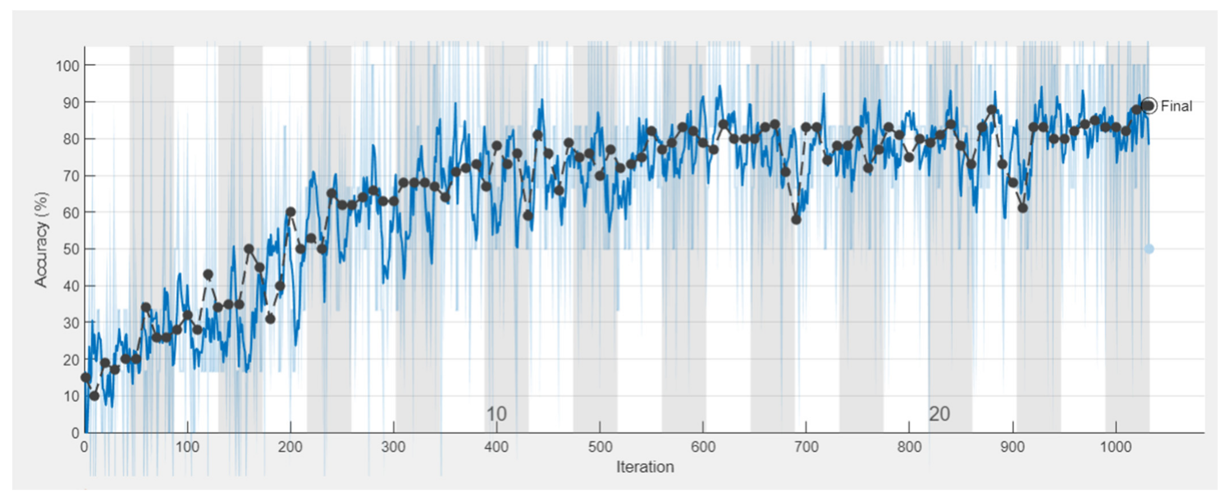
The network training with current signals required more iterations to reach convergence with respect to the case with three classification classes. The steady validation accuracy was about 85%, which is lower than that obtained for the radial flux signal but higher than that achieved for the current signal in the first tests.

Figure 11 shows the training and validation progress of the seven classes of current signal classification. The maximum number of epochs was set to 24 and the process lasted about 7 min. The confusion matrix is shown in Figure 12.

As can be seen from Figure 12, the most misclassified classes are those with the generalized roughness defect. Also, the baseline class was sometimes classified incorrectly as “BF Step 2” (Bearing Fault Step 2).

4.2.3. Mixed-Signals Approach

A network trained using both the current and the flux signal is presented in this section. The number of images used was twice the number of images used in the single-signal analysis. The maximum number of epochs was set to 24 while the weight and bias learning factor was increased to 25. The validation accuracy reached 89% and convergence occurred in about 18 epochs, as visible in Figure 13. The time for the computation was about 13 min.

The same test was repeated with the decimated data. With these data, the validation accuracy was reduced by about 13% (it reached 76%), with a rapid convergence of about 10 epochs. The confusion matrices of both the cases of non-decimated and decimated data are presented in Figure 14.

As can be seen from Figure 14, the only misclassified class for the non-decimated data was the “BF Step 1”, with 50% misclassified images. The total test accuracy was 95%. For the decimated data, many classes were misclassified, for example “Bas”, “BF Step 1”, “H12”, and “H45”. The total test accuracy for the decimated data was 81.2%. This could be interpreted with the fact that the network also sees patterns at a high frequency in the scalograms, so it could reach higher validation and test accuracies for the non-decimated data.

4.3. More Challenging Tests: LFTO as Additional Fault

Some tests were carried out with LFTO; this condition could simulate a rotor bar fault or a particular type of mechanical load, as introduced in Section 3. A double fault condition was simulated with the use of signals from a machine with a bearing defect and an oscillation load torque, as also discussed in [49].

In this case, only the stator current signal was used. The LFTO condition constituted of a sinusoidal torque oscillation of 0.5 Hz summed over a constant load torque. Due to a lack of data measured with LFTO, only four classes were used, i.e., the classes of the localized fault at four different angular positions, without the baseline class.

Decimated and non-decimated data were compared in the computations. Moreover, the analogous four classes with localized faults without LFTO were classified through the neural network for direct comparison between the single and double fault conditions. In the first instance, the single fault conditions and the double fault conditions were fed separately into the neural network; in the second instance, all eight classes were fed together into the network for the same classification task.

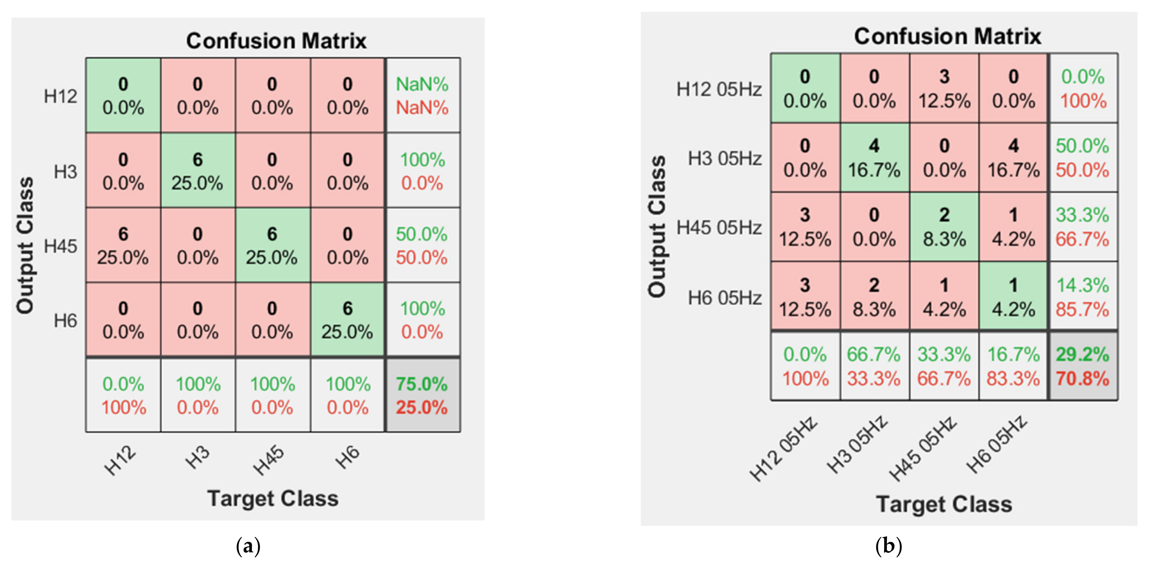
4.3.1. Tests with Four Classification Classes and LFTO

The data signal with LFTO and those without LFTO were fed into the network separately to see how much the double fault condition “disturbs” the classification process. It should be noted that validation accuracy changes greatly from non-decimated to decimated data. Accuracy also varies between the validation dataset and the test dataset. As for the previous tests with the current signal, a maximum number of 24 epochs was set for the process, whilst all other parameters were kept the same as before. The results are shown in

Table 5. Validation and test accuracy for the bearing fault and LFTO condition compared with the single fault condition data.

Case	Decimation	Validation Accuracy	Test Accuracy
Bearing fault + LFTO	NO	65%	83.3%
	YES	56.7%	29.2%
Bearing fault	NO	98.33%	95.8%
	YES	75%	75%

.

As can be seen from Table 5, the double fault condition introduced more difficulties in the classification process, as expected. The data with a full (non-decimated) frequency spectrum gives better classification results. In particular, with the decimated data, difficulties were especially encountered in recognizing the H12 class (for both the single and double fault conditions) and the H6 class (in the case of double fault), as shown in Figure 15.

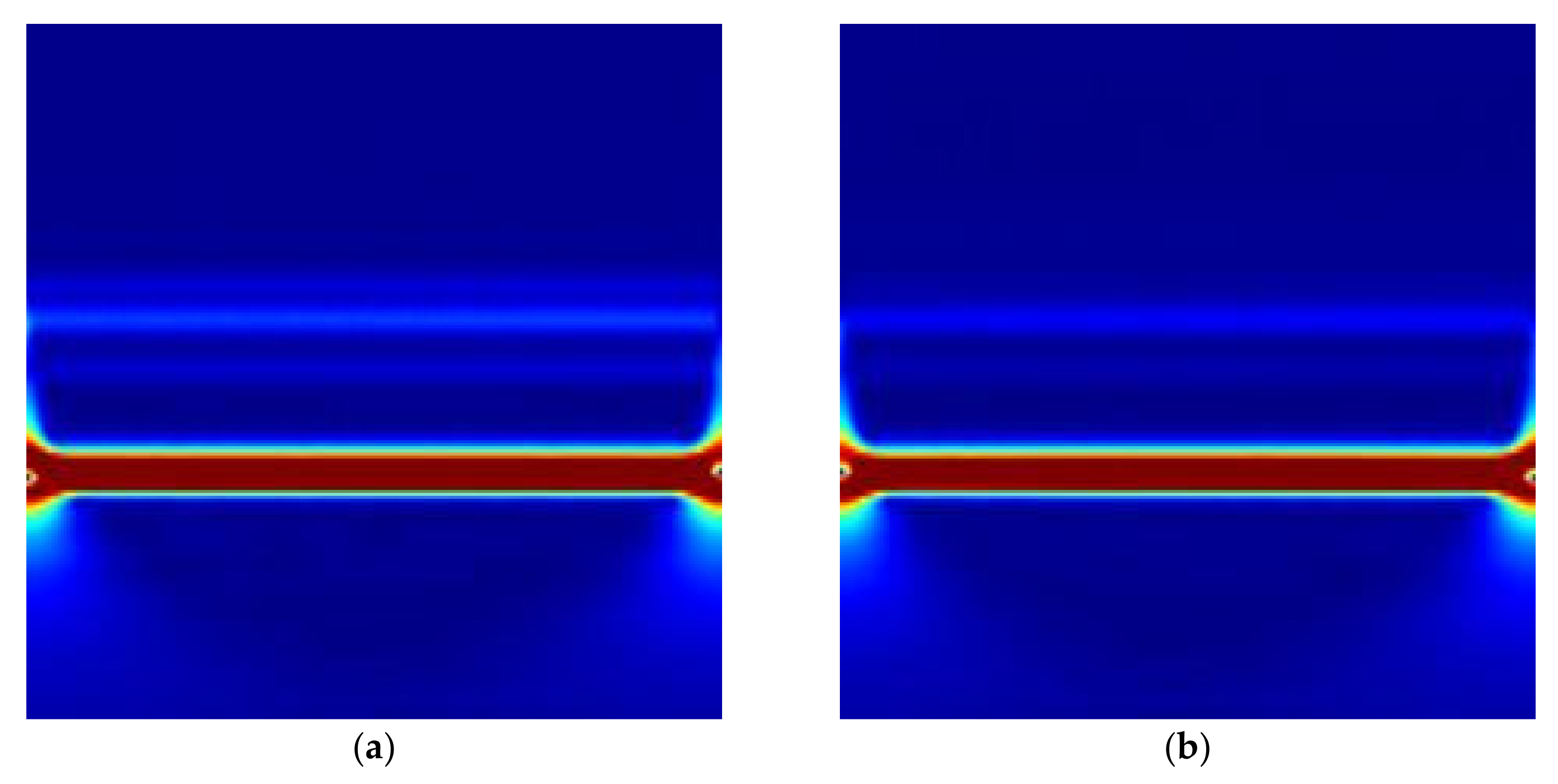
It should be noted that, in the case of LFTO, the electromagnetic signal’s images generated with the CWT do not show characteristic patterns easily visible to the naked eye, as is possible to see in some of the vibration spectrogram images presented in [25], so it should also be quite difficult to distinguish the scalograms obtained with the double fault compared to the single fault condition for the neural network. Two sample images from the decimated data are reported in Figure 16.

4.3.2. Tests with Eight Classification Classes and LFTO

The test presented here was performed by mixing the data for the single fault with the data for the double fault, in the case of non-decimated data. With this setup of eight classes, it was possible to understand if the network correctly saw differences between the single and double fault condition classes.

4.4. Tests with STFT

For the sake of a comparison between scalograms and spectrograms, in this section, the STFT was applied to generate the spectrograms.

With the STFT, data relating to the localized bearing defect, with and without the second fault condition due to LFTO, were fed into the network, separately or jointly, to have a direct comparison with the result obtained in Section 4.3. Only the data from the current signal were used, since only this signal had been measured in the case of LFTO.

The spectrogram generation was obtained with the same data as presented in Section 4.3, but the data were mean-var normalized and decimated with a decimation factor of 20 or 30, since this has given better classification results previously (tests from non-decimated spectrograms have been omitted due to their very low classification accuracy). The number of images generated for each class was kept to 60, the base sampling frequency was 120 kS/s, and the base input segment length was 100,000 samples, as in the previous tests presented.

The input decimated frequency and input signal length with the parameters for the spectrograms’ generation are shown in

Table 6. Parameters chosen and size of the spectrogram images generated.

Decimation Factor Used	Decimated Sampling Frequency	Number of Samples (Decimated)	Window Length	Overlapping Samples	Number of DFT Points	Dimension of the Spectrogram Generated
Input Segment			Parameters for the Spectrogram Generation
20	6 kHz	5000	750	739	452	227 × 387
30	4 kHz	3333	750	739	452	227 × 235

.

The spectrogram was generated through the use of the MATLAB “spectrogram” function. The input parameters were the window length, the overlapping samples, the number of DFT points, and the (decimated) sampling frequency used; these parameters are shown in Table 6. With this setup, the Hamming function was used for the windowing of each 750-point window by default. This function returned a matrix representing the Power Spectral Density (PSD) of each segment.

After generating the spectrograms, a conversion into dB values was performed; to convert into dB values, a small constant “epsilon” value was added to the matrix element values in order not to have problems with the logarithmic calculation of numbers very close to zero. Finally, the .jpg images were generated using the “imwrite” function with the “jet” colormap and stored in dedicated folders. All the images were resized to dimensions of 224 × 224 through the “imresize” MATLAB function, which uses bicubic interpolation of the data. 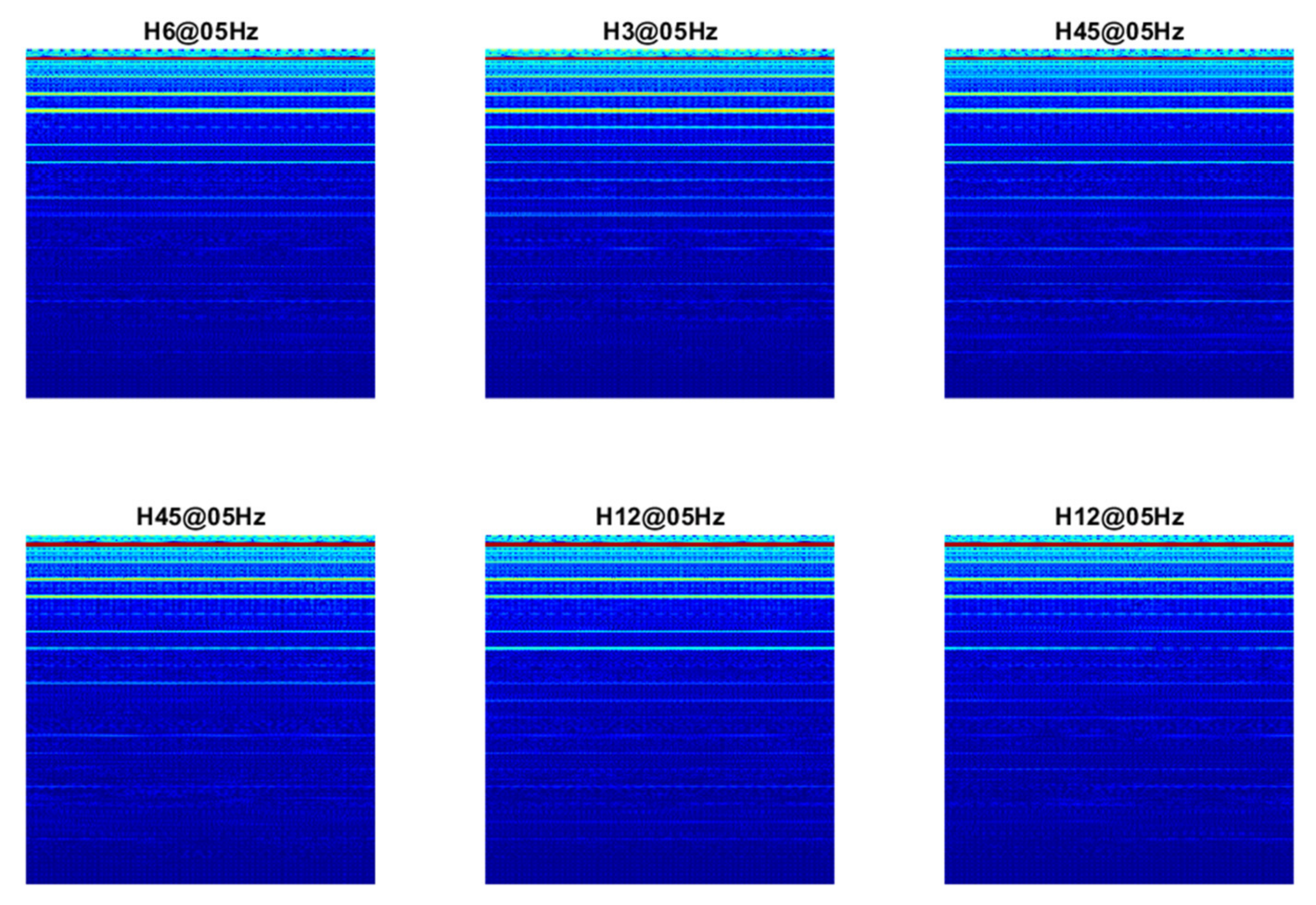In Figure 17, some spectrograms relevant to the current signal with the LFTO condition are shown.

Tests were carried out with four classes per setup (the four localized faults without LFTO and the four localized faults with LFTO) and with a setup of eight classes in which all the cases considered were fed together into the network, as previously in Section 4.3.

4.4.1. Tests with Four Classification Classes and LFTO

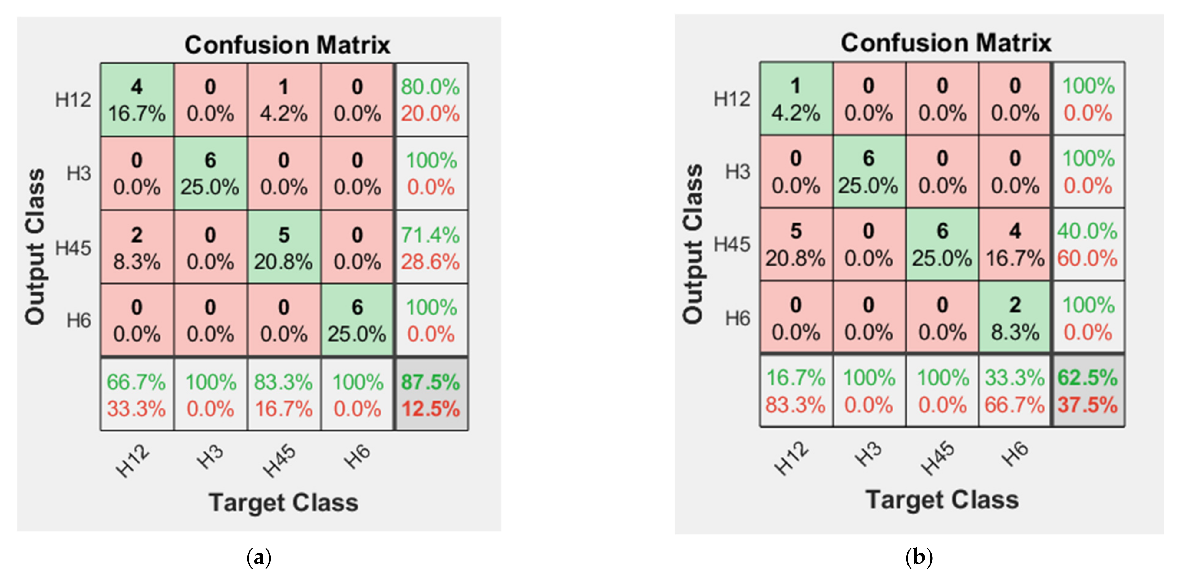
The validation and test accuracies for each setup of four classes are reported in

Table 7. Validation and test accuracy for the two classifications with four classes each (spectrogram images).

Case	Decimation Factor	Validation Accuracy	Test Accuracy
Four localized bearing faults + LFTO	20	75%	79.2%
	30	61.7%	62.5%
Four localized bearing faults without LFTO	20	90%	87.5%
	30	91.6%	87.5%

for the various cases. The confusion matrices for the cases with a decimated factor of 30 are shown in Figure 18.

As can be seen from Table 7 and Figure 18, by comparing with the respective Table 5 and Figure 15, the accuracies reached with the spectrogram images tended to be better than those achieved with the scalograms, in the case of decimated data.

4.4.2. Tests with Eight Classification Classes and LFTO

In this case, for the sake of brevity, only the result with a decimation factor of 20 is reported. The eight class setup with the spectrograms gave a classification accuracy of 75.8%. The confusion matrix for this case is reported in Figure 19.

In this case, it should be noted that the test accuracy was lower than that found in the previous section (see Figure 20); in fact, the test accuracy here was 66.7% instead of 91.7% as for the classification based on scalograms.

The validation accuracy achieved was about 90% and the convergence was reached in about 18 epochs. The confusion matrix for this setup is shown in Figure 20. Note that in Figure 19 and Figure 20 the names of the rows and columns correspond to the denotations (acronyms) of the different classes.

5. Discussion

In this work, an analysis of the stator current and radial stray flux signals for the diagnostics of an induction machine with bearing defects is presented. All the data were collected by performing laboratory tests.

The analysis of the signals was obtained through the use of GoogleNet, a deep Convolutional Neural Network (CNN). The network was adapted for the classification of the various bearing fault images through the use of the transfer learning technique. This technique substantially consists of retraining a pre-trained network (i.e., GoogleNet, a network trained for the classification of 1000 classes of object images) only in the last fully connected layers, with a reduction of the number of output classes. The network keeps the feature extraction abilities learned in the first layers in the full training process, but it can adapt these abilities for the classification of new classes of input images (i.e., the time-frequency transformations of the electromagnetic signals coming from the measurements on the machine).

The bearing defects considered were generalized roughness (with two severity levels) and localized defects in the outer ring (in four different angular positions). Moreover, tests with both a localized defect and Low Frequency Torque Oscillation (LFTO) were also analyzed. The raw data were converted into a 2D time-frequency domain through the use of the Continuous Wavelet Transform (CWT) and the Short Time Fourier Transform (STFT). Comparison between the data transformed with these two techniques were reported in Section 4.

Various types of tests are presented in this paper. The first ones considered three classes, i.e., the baseline (healthy) condition and the faults with generalized roughness. These tests were carried out on both the current and stray flux signals, with the use of the wavelet transform. In these tests, the stray flux signal gave better classification accuracy than the current signal.

Other tests were carried out with the addition of the bearing’s localized defect data to the baseline and generalized roughness data. With these tests, the stray flux signal gave a validation and test accuracy of 100%, while for the current signal, an accuracy of about 80% was reached but with a maximum number of epochs in the training process augmented to 24. Current and stray flux signals were then mixed together, reaching a validation accuracy of about 90%. In these tests, the data with a full sampling frequency and with a decimated frequency were used, usually reaching better classification accuracy with the non-decimated data.

Subsequently, classification tests were carried out with the localized defect data classes with and without the LFTO condition. These tests were performed with the current signal only, due to a lack of data measurement of the stray flux. The tests were carried out with the use of scalogram and spectrogram images, coming from the two different time-frequency domain transformations. Moreover, the double fault condition characterized by the presence of the localized defect in the bearing and the LFTO were analyzed jointly and separately from the single fault condition, that is, the signal of the defected bearing without the torque oscillation. So, the tests with four classes (representing the single or double fault condition of the four localized defect signals) were carried out, and finally the eight classes classification of the single and double faults considered jointly were reported. In these final tests, attention was paid to the differences in classification accuracies of the network with data transformed with the CWT, i.e., the scalogram images, and with the STFT, i.e., the spectrogram images. The results show that the validation and test accuracy can change for the four class setups and for the eight class setups. For the four class setups, better results were reached with the spectrogram images (test accuracies of up to 87.5%), but with the more complex eight class setups, better results were reached with the scalogram images (test accuracies of up to 91%). It should be noted that, with the scalogram images, a non-decimated signal gives better classification accuracy, while with the spectrogram images, a bigger decimation factor can generate images that give better classification accuracy.

6. Conclusions

The results presented in this paper have demonstrated the ability of electromagnetic signals coming from an induction motor in detecting different types of bearing faults and mechanical anomalies due to the load. This outcome agrees with several papers published recently, although with some differences; in particular, with respect to [12], the external stray flux in the present study proved to be more efficient than the current in detecting bearing faults. This discrepancy could be due to the fact that in this work, a small motor was taken into account, in which the stray flux sensor was installed very close to the defected bearing; on the contrary, the large size of the motors analyzed in [12] does not allow the installation of an external sensor sufficiently near to the bearings. In any case, as suggested in the literature, we can confirm that the measurement of both current and flux signals may be useful to increase the diagnostic efficiency for all sizes of motors.

Regarding the use of Convolutional Neural Networks, the obtained results show their capacity to automatically discriminate the bearing faults and with respect to the healthy condition. The comparison between the use of scalograms or spectrograms as input to the network has shown that they can give different classification accuracies and the best choice cannot be defined absolutely; therefore, an evaluation of both methods could be effective for an automatic diagnosis of the faults.