Article

Multi-Parametric Imaging of Etruscan Chamber Tombs: Grotte Di Castro Case Study (Italy)

1
Istituto Nazionale di Geofisica e Vulcanologia, Via di Vigna Murata 605, 00143 Rome, Italy
2
Independent Researcher, Via Casilina 33, 00030 Colonna, Italy
3
Museo Civita di Grotte di Castro, 01100 Viterbo, Italy
*
Author to whom correspondence should be addressed.
Appl. Sci. 2021, 11(17), 7875; https://doi.org/10.3390/app11177875
Submission received: 5 August 2021 / Revised: 24 August 2021 / Accepted: 25 August 2021 / Published: 26 August 2021
(This article belongs to the Special Issue Integration of Methods in Applied Geophysics)

Abstract

:

Featured Application

We identify undiscovered archeological burials through a multi-parametric approach, which includes electrical resistivity tomography, capacitive resistivity and ground-penetrating radar methods coupled with the novelty of Radon in soil measurements. This approach has proved to be a fast and easily deployable tool for mapping burials in a particular geological context.

Abstract

A multi-parametric approach that involves the use of different geophysical methods coupled with geochemical data allowed us to identify undiscovered archeological burials in a funerary area of the Grotte di Castro Etruscan settlement. In particular, we tested the suitability of the capacitive resistivity method and the presence of Radon in soil for the identification of burials calibrating their outcomes over coincident survey profiles with standard geophysical techniques routinely applied for archaeological prospections. Soil Radon data were acquired both in a grid and along a profile to highlight anomalous gas concentrations, whereas electrical resistivity and ground-penetrating radar measurements were conducted on overlapping profiles to depict the electrical and electromagnetic subsurface distribution. Data integration showed a series of anomalies, suggesting the presence of multiple burials starting from a depth of approximately 1.5 m below the terrain surface. Slight anomalies of Radon in the soil were found to correspond to most of the recovered geophysical ones. Our results pointed out the effectiveness of geophysical method integration in archeological prospecting with the novelty of the joint use of Radon in soil measurements and capacitive resistivity tomography. The latter provided reliable results and can be considered as a standalone technique in archaeological surveys.

1. Introduction

Grotte di Castro is a medieval (IX-X c.) village within the Viterbo province, approximately 100 km north-northwest of Rome, close to the border between Lazio, Toscana, and Umbria. The study area is a portion of the Vigna la Piazza necropolis, one of the several funerary areas (Figure 1) pertaining to the Etruscan settlement of Civita, the remains of which occupy a wide tuff plateau rising 0.5 km southeast of the modern village [1]. Herein, we present the results from a multi-parametric research approach, which involves the use of geophysical and geochemical data with the aim of mapping new archeological features over a portion of the Vigna la Piazza necropolis that is located amongst a volcanic environment (Figure 1). The geophysical and geochemical study of buried structures in Vigna la Piazza relies on the possible presence of empty, partially empty, or recently filled voids excavated inside the tuff ridge. The contrast between soil/air/soil interfaces makes electromagnetic (EM) and electric methods suitable for their detection.
Geophysical methods play an important role in the investigation of shallow buried remains and aid in focusing the wide berth of archeological excavations [2,3]. The effectiveness of any geophysical method depends on (i) the existing contrast in the physical properties that allows characterization of the target and host media (i.e., electrical, EM) [4], (ii) the environmental setting, and (iii) the logistical constraints that may hamper or limit the geophysical survey (e.g., in urban areas) [5].
Recently, multi-parametric geophysical surveys have become a standard approach as they provide a higher level of accuracy in data interpretation compared to a single technique. Regarding the archeological investigation, the joint use of geophysical methods based on detecting contrasts in the dielectric constant, such as ground-penetrating radar (GPR), in the resistivity distribution is similar to those measured by electrical resistivity tomography (ERT) or in the magnetic susceptibility through magnetic method (MM) are the most used to image buried remains [6,7,8,9,10,11,12].
Among them, the capacitive-coupled resistivity method (CCR) is less present in the archeological literature, even though it permits the mapping of the subsurface resistivity distribution over large areas in a relatively short time as capacitive electrodes can be towed over the surface [13,14,15].
The application of geochemistry as a tool to locate and delineate archaeological sites [16,17] or to interpret archaeological soil features [18,19,20] and buried cavities [21] reported, till nowadays, a limited understanding of the link between soil chemistry and the presence of archaeological remains. This aspect is witnessed by the low number of peer-reviewed studies that report on the use of geochemistry to map archaeological targets compared with those using geophysical methods, remote sensing, and coring [22].
Geology modified from the geological map of Regione Lazio (http://dati.lazio.it/catalog/it/dataset/carta-geologica-informatizzata-regione-lazio-, accessed on 25 July 2021). The geological units reported in the legend are: Alluvial gravel, sand, and clay (A); Scoria and lapillus (B); Oversaturated lava and laccolith (C); Oversaturated and undersaturated Lava (D); Tuffs, mainly litoid (E); and Stratified and earthy tuffs (F). The inset shows the Roman Volcanic Districts modified from Manca et al., 2017 [23]. The solid-black dots 2 through 15 indicate the locations of the main necropolis in the area, while dot 1 indicates the position of the Civita plateau, with detail of the defended perimeter [24].
However, isotope geochemistry can significantly contribute to archaeological research and investigation. A wide range of elements and materials can be analyzed to provide insights into the age, diet, mobility, climate, and provenance of a settlement with important implications in providing useful archaeological hypotheses [25]. Moreover, it was demonstrated that constraints on the shape and the orientation of graves could be obtained in a very fast and reliable way by sampling the Rn-222 radioactive gas isotope in the Etruscan necropolis of Tarquinia (Italy) [26].
Furthermore, integration between Radon (Rn) measurements and geophysical methods has been successfully applied to locate the Chinese Emperor Qin Shi Huang Mausoleum underground palace [27].
In the Grotta di Castro area, the suitability of the method is ensured by the presence of volcanic tuff, which is known to naturally emit Rn into the atmosphere [28]. The continuous emission of Rn involves its accumulation, especially in empty hollows and in the absence of migration pathways [29]. In light of this, Rn in soil measurements was tested as a complementary technique for the individuation of archeological burials. Data were acquired over a regular grid and a profile in overlap to the ERT, CCR, and GPR surveys in order to check for anomalous values and their relation to the geophysical anomalies.
In addition, this study also reports on the comparison in terms of data resolution and output models between CCR and standard high-resolution techniques (GPR and ERT). The main strength and weakness points of each geophysical method were considered, and the use of Rn methodology as an alternative method to locate relevant burial targets was evaluated. The obtained results of combining data from different methods show a relatively good correlation regarding the mapping of the subsurface archeological structures. Even the Rn survey shows a good match with other standard geophysical methods.
A secondary goal of this study case was to provide the “Soprintendenza Archeologica Belle Arti e Paesaggio” with a non-invasive and reliable investigation strategy for approaching this type of survey in similar application contexts [14,30]. On this topic, the recorded data and models were overlaid onto a high-resolution (1 pixel = 0.05 m) digital surface model (DSM) and an orthomosaic image of the whole study area obtained by a photogrammetric survey. The latter was carried out using a low-angle, 9 m tall, pole-mounted mirrorless digital camera and the “Structure-from-Motion (SfM)” photogrammetry technique. To scale the images, we employed a dual-frequency geodetic GPS/RTK receiver STONEX A6000 to measure the coordinates of a set of reference ground control points (GCPs) in the investigated area. GCP positions were estimated in real-time using the RTK technique, obtaining 1–2 cm accuracy with respect to the reference GPS station TOLF, which belongs to the GNSS network of the Istituto Nazionale di Geofisica e Vulcanologia (Avallone et al., 2010) and pertains to the ITALPOS network (https://hxgnsmartnet.com/en-gb/. Accessed on 25 June 2021) for real-time positioning services. The obtained DSM (4 points/cm2) and orthophoto resolution was in the order of 5 mm/pixel.

2. Materials and Methods

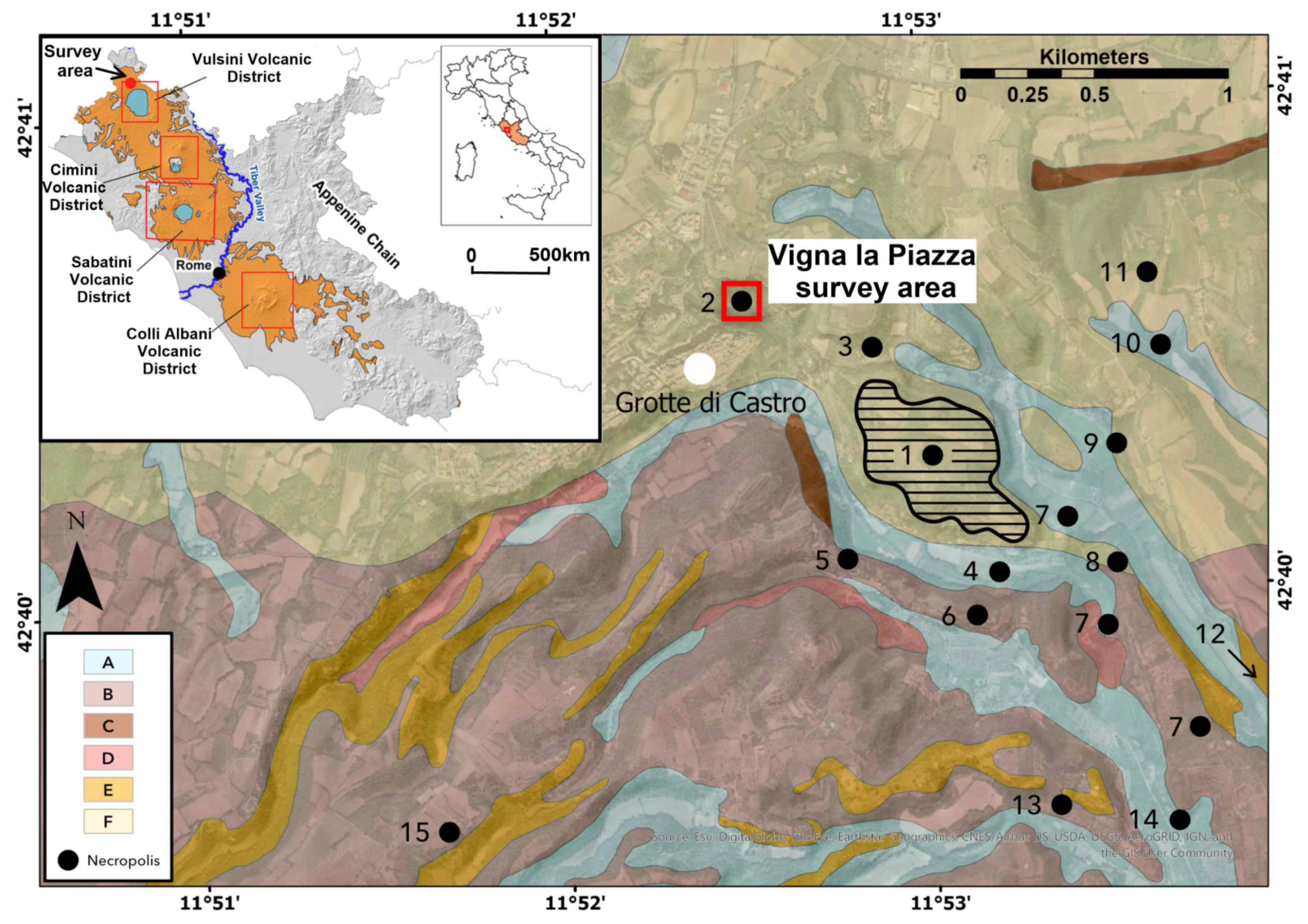
2.1. Geological and Archeological Settings

The study area is located a few kilometers north of the Bolsena Lake in the Vulsini Volcanic District, which is characterized by four emission centers that were active 600,000–100,000 years ago, and are now represented by the caldera collapses of Bolsena Lake, Montefiascone, Latera, and Vepe [31]. The study area lies on a tuff ridge, which is the result of the deposition and subsequent weathering of volcanic ashes from the Latera Complex [32,33]. In the study area, the chemical composition of the rocks is mainly characterized by potassium, rubidium, thorium, uranium, and volatile elements, such as chlorine and fluorine. The origin of the K-rich magmatic activity is related to the development of the eastern extensional structures of the Tyrrhenian basin, which occurred between the orogenic belt of the Apennines and the slow spreading center of the Tyrrhenian Sea [23].
The Grotte di Castro area and its surroundings have been of interest to human occupation since the early Middle Paleolithic (35–100 ka), wherein the earliest evidence of human occupation are Musterian lithic assemblages [34]. At the beginning of the Archaic Age, the settlement of Civita acquired relevance by becoming, and was reconstructed to be [24], the northernmost point of the defense system organized and kept in use by Volsinii from the VI to the III century BCE. During the VI century, the settlement occupied part of the upper hillside with a total area of approximately 24 ha and remained seemingly prosperous, not without inconsistencies, until the end of this period. Aside from the Casali Centocamere and Pianezze, the Vigna la Piazza necropolis is one of the most important Etruscan funeral sites among those found and investigated in the immediate surroundings of the Civita plateau. It lies less than one kilometer northwest of the northernmost edge of the plateau at 427.2 m ASL on the SP48 road, which connects the Grotte di Castro with the Bolsena lakefront area. Approximately 30 m west of the necropolis, a segment of an ancient “tagliata tufacea”, a path running in a man-made tuff gorge, testifies to the Etruscan road system connecting the Civita plateau with the surrounding necropolis and wider landscape. This necropolis was in use from the end of the VIII century to the beginnings of the V century BCE, thus making it the most ancient of those around Civita. It is characterized by both individual burial sites in simple pits or pits with lithic sarcophagi and multiple burials within rock-cut chamber tombs pertaining to the most characteristic local types (Figure 2). These tombs are formed by a dromos (access corridor) and an atrium (central room), providing access to the tablinum and cubicula funerary rooms [1,24,34]. This particular tomb typology was chosen for the present study because of the strong geophysical and geochemical signature given the expected contrast between the rock-cut chambers walls and the infill (either empty or filled with soil).

2.2. Electrical Resistivity Data Acquisition

Electrical methods reveal information regarding subsoil material and buried structure architecture through the analysis of the resistivity distribution (ρ, expressed in Ohm.m) measured along survey profiles. In this study, ground resistivity data were acquired using two different electrical resistivity tomography methods: CCR and ERT.
The CCR instrumentation (OhmMapper powered by Geometrics) consists of a multi-receiver array (five receivers) with a 5 m dipole-dipole transmitter and receiver cables [35] and a constant rope length of 5 m. This configuration was used to measure the 2-D subsurface resistivity distribution down to a depth of approximately 5 m along three transects: CCR1, CCR2, and CCR3 (Figure 3). The measured voltage at the receivers is a function of the ground resistivity between the receiver and transmitter dipolar cables [36], while the depth of the investigation is generally dependent on the number of receivers employed and the maximum transmitter and receiver distance [37]. Data processing included filtering to remove outliers and smooth the raw voltage data. Then, the de-spiked and filtered data were inverted via a regularized inversion algorithm and smoothness constraints [38] to obtain the 2-D distribution of the terrain resistivity. Due to the limited size of the survey area and the presence of scattered vegetation, it was not possible to cover the area with multiple-parallel profiles to extract the 3-D resistivity distribution. The CCR1 profile was recorded in the northern part of the study area, along a small northwest-southeast oriented trail. The CCR2 profile is located on a small flat area above the main paved road upon which the CCR3 profile was acquired.
The ERT method was used to obtain a high-resolution resistivity model along the CCR2 profile and to cross-check the CCR output. We deployed an array of 48 steel electrodes (1 m apart) for a total profile length of 48 m using a georesistivimeter Syscal R2 (IRIS Instrument). We injected a bi-polar square pulse of 250 ms, using a 100 V energy source, to measure n. 714 quadrupoles in a dipole–dipole configuration, which is sensitive to horizontal changes in resistivity and thus suitable to reconstruct shallow subsurface vertical structures. Data processing consisted of removing low voltage data and evident spikes in the raw apparent resistivity data.
Since we did not acquire reciprocal measurements, we use resistance contact, current and the voltage levels as noise indicators to clean the dataset; data quality was instead estimated, taking into account the number (N) of stacks (i.e., repeating the same measurement N times) required for each measure and thus the error was evaluated from the standard deviation for each of the recorded data. We used the algorithm proposed by Loke and Barker (1996) [38] for the 2-D data inversion. The ERT electrodes and the CCR profiles’ topography were extracted from a high-resolution DSM built using a photogrammetry survey.

2.3. GPR Data Acquisition

GPR is an electromagnetic technique that detects the location of objects or interfaces that are buried beneath the shallow portion of the subsoil and characterized by their dielectric properties. In some soil types, such as those characterized by a high content of mineralized water (i.e., clay), or those derived from volcanic rocks or otherwise high in iron or metallic content, conduction and dielectric effects can cause the absorption of EM radiation, reducing the effectiveness of the GPR method [39,40,41].
Herein, the outcropped volcanic unit is mainly characterized by stratified and friable volcanic tuff and is thus suitable for the GPR method. The survey was conducted during the summer to reduce the impact of moisture content. Moreover, void detection is also one of the most suitable targets for this kind of investigation, and the Etruscan burial roofs were expected to occur at a relatively shallow depth (approximately 2 m). Based on these considerations, we recorded three GPR profiles (labeled GPR1, GPR2, and GPR3 in Figure 3) using a GSSI Sir3000 instrument equipped with a 400 MHz central-frequency antenna. The main acquisition settings were as follows: range, 70 ns; vertical sampling, 512; horizontal sampling, 100 scan/m (120 scan/s); 16 bit dynamic. Data post-processing included the application of vertical and horizontal band-pass filters, deconvolution, gain equalization and migration. Reflection arrival times were converted to depth using an averaged EM wave speed of 0.11 m/ns, which corresponds to a dielectric constant of ɛ = 7.5. The “ɛ” starting value was calculated by measuring the two-way travel time (TWT) of the reflections generated from the top of the EB1 excavated burial (Figure 3). This value was integrated using velocity analyses on diffraction hyperbolas occurring along the profiles and was found to be consistent with those proposed in the literature for the same soil type [42,43].
The measured GPR data were georeferenced by linking a geodetic GPS receiver (Topcon GB1000) and using a survey wheel to obtain a more rigorous determination of scan spacing.

2.4. Radon and Thoron Soil Gas Data Acquisition

Radon is a noble gas and is the only naturally occurring radioactive gas. It has three isotopes: 222-Rn (Rn, half-life: 3.8 days), 220-Rn (Th, half-life: 55 s), and 219-Rn (Attinon, An, half-life: 3.96 s). Rn is a short-lived decay product derived from the 238-U decay series, while Th derives from the 232-Th decay series. Because of its low mobility, it needs a gas carrier, such as CO2, to move from underground to the surface. The relatively short half-life of Th makes it useful in discriminating sectors with very fast soil-gas transport and/or Th-rich mineral outcrops. Thus, Rn soil gas measurements were performed along a regular grid of 20 samples (labeled from GC1 to GC20), approximately 2 m apart in order to cover the flat area (approximately 300 m2) where the CCR2, GPR2, and ERT profiles were acquired (see Figure 3). Moreover, an additional nine samples were collected along the CCR1 profile (labeled SGC1 to SGC9). The soil Rn and Th measurements were carried out using a RAD7 Durridge® radon meter. The RAD7 measures concentrations of both 222-Rn (Rn) and 220-Rn (Tn) in the gas phase by exclusively collecting Rn and then counting the alphas emitted by the decay of their respective daughter nuclides 218-Po (t1/2 = 3.04 min) and 216-Po (t1/2 = 0.145 s). The soil Rn and Th were pumped from the ground at a depth of 40–50 cm using an internal pump. A desiccant (drierite) trap and an inlet filter were used to protect the detector ionization chamber from reaching a soil humidity greater than 10% [44]. The Rn and Tn measurements require approximately 15 min of pumping in the field in order to reach equilibrium with the measured daughter nuclide 218-Po. The acquired data were statistically and graphically processed to identify the geochemical lineaments, background values, and anomalies. An objective approach to the anomalous threshold estimation was obtained using probability graphs [45]. This procedure entailed approximating segments of a probability curve (or identifying inflection points) by straight lines and then selecting threshold values at abscissa levels that corresponded to intersections of these “linear” segments. In the simplest case, a single threshold would define two populations (background and anomalous values). However, if the two populations are not clearly separated, they may overlap in an interval defined by two bounding threshold values. Classed post maps of Rn, Th, and their ratio were developed for data visualization and to study spatial patterns. These maps group the data into discrete classes that represent different populations (i.e., background, low anomalous values, high anomalous values, and outliers) distinguished on the probability plots.

3. Results

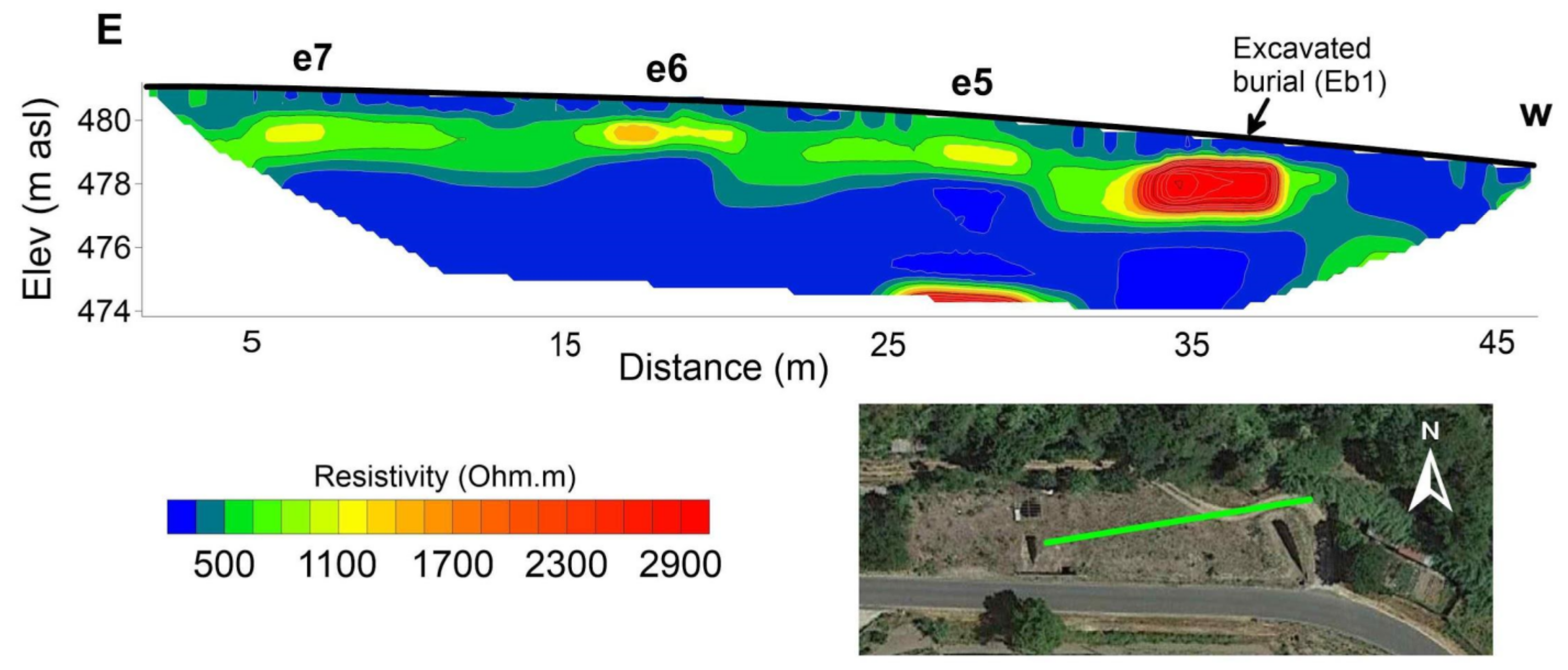
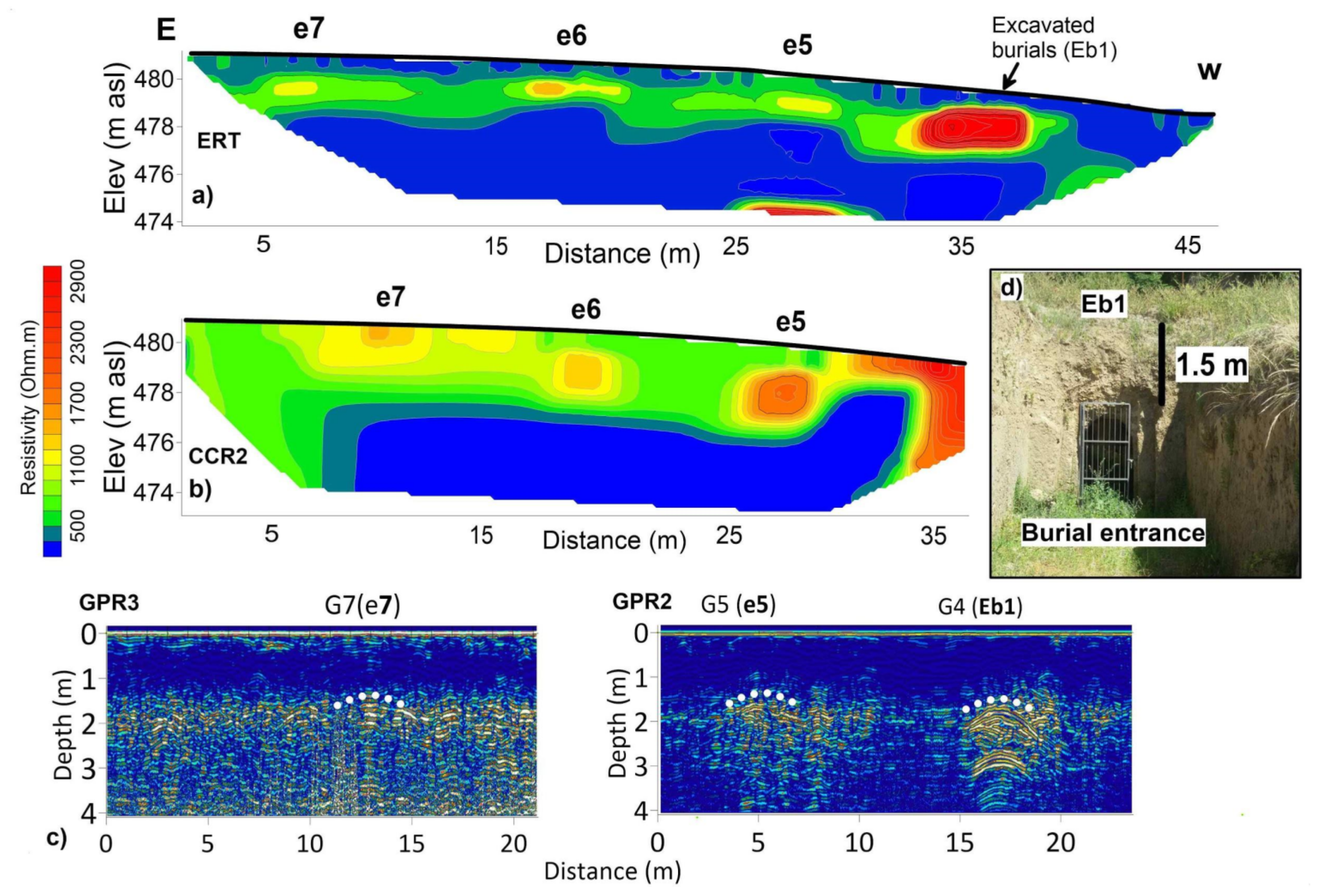
3.1. Electrical Resistivity Results
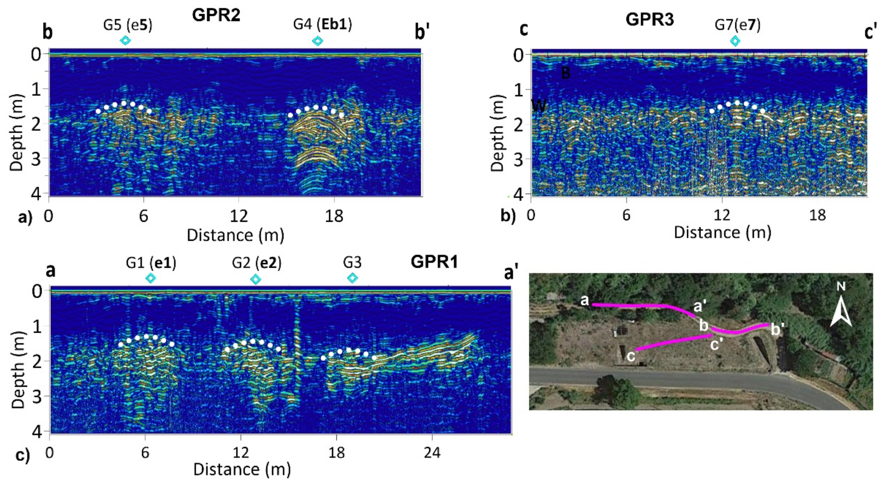
Figure 4 shows the resistivity profiles obtained from the inversion of the CCR measurements. The CCR2 profile (b-b’ in Figure 4a) was recorded by crossing the excavated burial site Eb1 (Figure 3) to obtain a resistivity reference signature of the investigated targets. This burial was located on the border of the area, which was very close to a metallic fence that prevented the center of the capacitive dipoles from being towed over it.
Nevertheless, the void presence was still well recognizable in the eastern margin of the profile where high resistivity values (ρ > 2500 Ohm.m) occur. Because of its marginal position, the Eb1 burial could not be correctly reconstructed by the inversion algorithm. Observing the distribution of resistivity values along the b-b’ transect, it was possible to separate the data into two sub-horizontal electrical units. A shallower unit, “A”, is characterized by ρ ranging between 500 and 900 Ohm.m and a thickness of approximately 4 m. This unit overlays a relatively lower resistivity unit, “B”, where resistivity values are lower than 350 Ohm.m. Within unit A, three shallow high-resistive anomalous spots occur, characterized by ρ values higher than 1200 Ohm.m (e5, e6, and e7 in Figure 4). These resistivity anomalies appear to be regularly spaced in the order of approximately 8 m and lie at a depth of approximately 1.5 m below ground level.
The CCR1 profile (a-a’ in Figure 4b) shows a similar subsurface resistivity setting, permitting the identification of the same two units, A and B, and shows three additional high-resistive anomalous structures.
In comparison with the CCR2 anomalies, these are slightly different in shape, spacing (approximately 10 m), depth, and output resistivity values (e1, e2, and e3 in Figure 4b).
The profile CCR3 (c-c’ Figure 4c) was recorded at a lower elevation on the paved road and it revealed completely different characteristics. According to the observed lower resistivity values, the resistivity color scale was centered on the unit B reference value (ρ ≃ 350 Ohm.m). This new scale highlights a low resistivity anomaly (e8 in Figure 4c) that coincides with the entrance of an additional excavated tomb (Eb2 in Figure 3). This anomaly is characterized by ρ values lower than 150 Ohm.m and shows sharp vertical contrasts that interrupt the imaged resistivity homogeneity of unit B.
To cross-check the recovered CCR resistivity anomalies, a high-resolution dipole–dipole array ERT survey (1 m electrode spacing) was conducted along the CCR2 profile (Figure 5). The ERT model confirmed the presence of the four resistivity anomalies whose positions are coincident with those recovered in the CCR2 profile. In addition, the model revealed the presence of a relatively thin (1 m) uppermost low-resistive layer (ρ < 200 Ohm.m) throughout the section, which is not as clearly identified.
With the ERT profile, we were also able to clearly identify the excavated burial (Eb1, Figure 3). The electrical image of Eb1 appears as a rectangular-shaped anomaly (approximately 2 m high and 4 m wide). characterized by high resistivity values (ρ > 2500 Ohm.m).

3.2. GPR Results

The GPR profiles conducted in Vigna la Piazza were performed to discover and locate possible, not-yet excavated, archeological remains, and to provide a constraint for the CCR and ERT recovered resistivity anomalies.
The rough site morphology and its status has impeded the acquisition of data onto 3-D grids, forcing us to perform only single lines.
Figure 6a shows the b-b’ radargram (GPR2 profile in Figure 3) that was recorded on top of the excavated burial site (Eb1). As expected, the anomaly (G4, x = 17 m), due to the presence of voids, is clearly visible in the radargram where both the roof and floor returned strong and continuous reflections (dashed white lines in Figure 6b). The Eb1 roof depth is 1.6 m below the surface and its floor at about 3.5 m, as observed using tape measures. The GPR-derived burial dimensions are 1.5 m wide and 2 m high. The absence of noticeable and diffuse wave scattering along the profile indicates that the host media has near-homogeneous dielectric characteristics.
A group of disarticulated strong amplitude reflections (G5, x = 5 m) occurred at the same depth as G4, separated by approximately 10 m. The distribution and amplitude of reflections suggest the presence of a partially void burial chamber that was probably refilled by fine-grained material. The latter is probably formed by weathered tuff, which has a very low dielectric contrast compared to the solid tuff. This particular configuration makes it impossible to correctly reconstruct the chamber geometry while allowing us to identify and locate it through the strong reflections from the void parts.
The c-c’ line (Figure 6b) was recorded on the flat area above the paved road and partially covered the first 20 m of the CCR2 profile (Figure 3). Here, the results were difficult to interpret due to the presence of more diffuse wave scattering occurring at a depth of approximately 1.5 m. At only one point (G7, x = 13 m), we observed an alignment of reflections stronger than the scatter average, with values similar to those recorded for the inferred voids aforementioned. Two additional spots, at x = 3 m and x = 19 m, showed similar reflections but were clearly disarticulated, thus making any interpretative hypothesis speculative.
The a-a’ line (Figure 6c) was recorded in the northern part of the study area along a small northwest-southeast oriented trail overlaying the CCR1 profile (GPR1 in Figure 3). According to the description and interpretation of the G4 anomaly, three evenly spaced and partially filled chambers were clearly recognizable at x = 6, 13, and 19 m along the profile. The G1 and G2 anomalies seem to be connected to the surface via small near-vertical holes visible at x = 5, 11, and 16 m.
Note that close to G3, a 7 m long, strong linear-shaped anomaly occurred starting at a depth of 1.7 m, becoming shallower to approximately 1.2 m below the surface. This anomaly was interpreted to be a small chamber or tunnel that is directly connected to G3 and elongated in the profile direction. The change in depth could be attributed to the change in the profile direction as a result of the trail path.

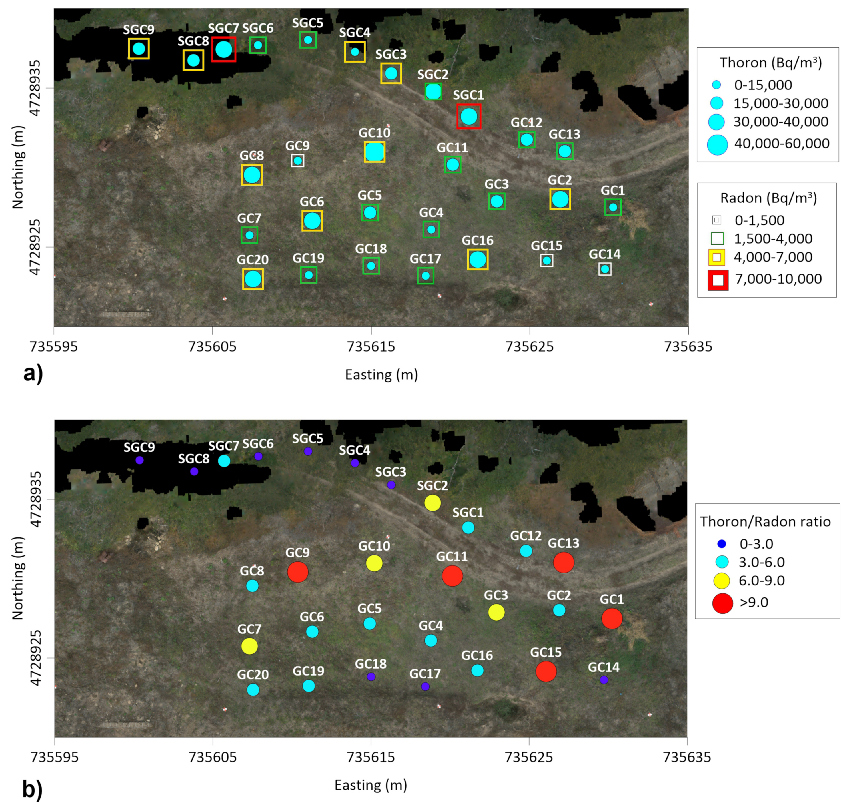
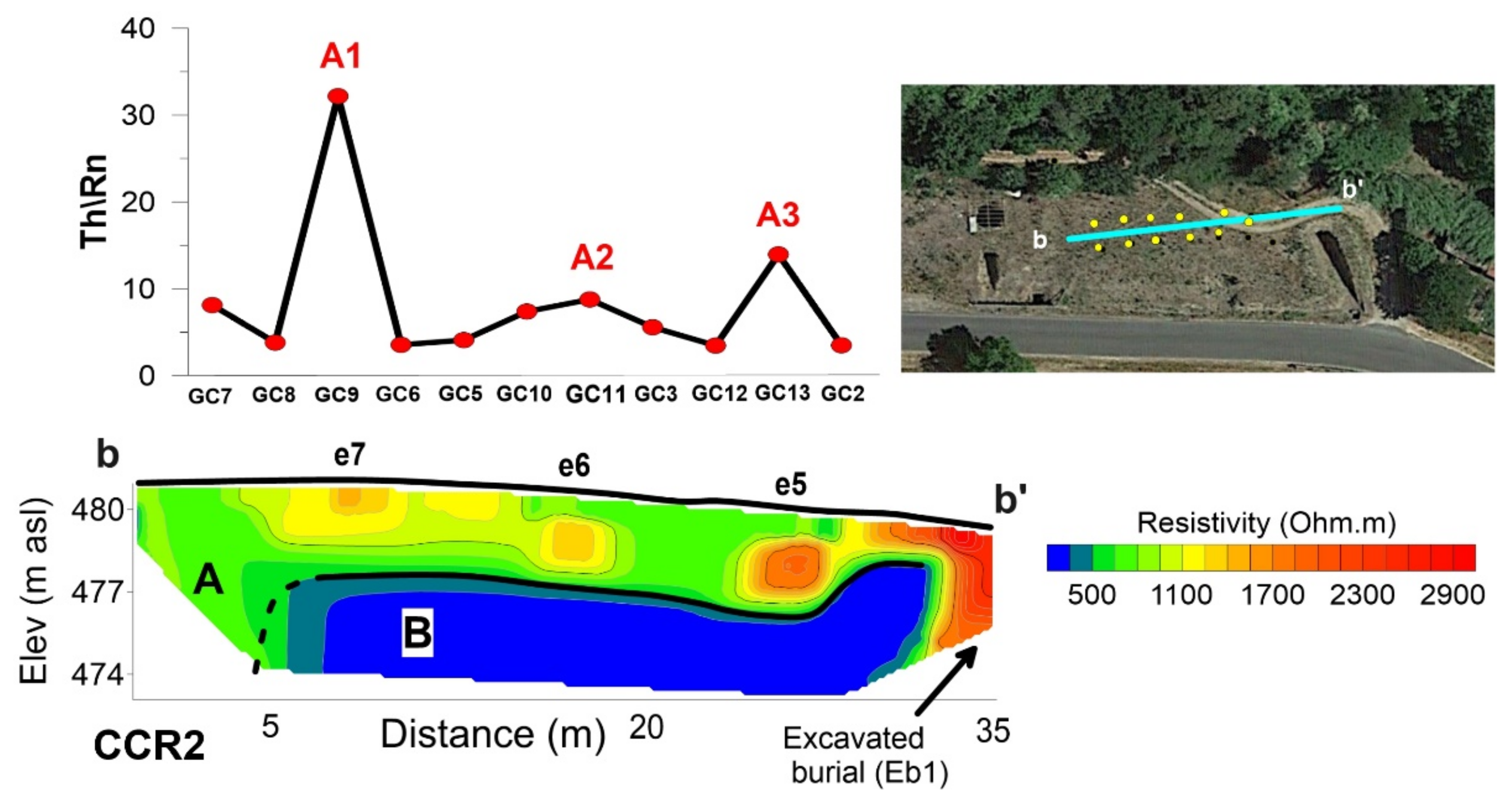
3.3. Radon and Thoron Results

Rn concentration anomalies must be analyzed site by site because of their dependence on local geological-structural settings.
According to [21] and [27], the presence of voids facilitates gas accumulation, which may propagate outward through fractures, enabling higher Rn mobility.
The gas concentration anomaly of a buried structure can be substantially observed in two different ways: (1) as a spot with a high concentration, in cases of an empty volume where gas accumulates due to the lack of air exchange with the atmosphere or (2) as a low concentration spot if the same volume is partially filled by soil, with no radioactive elements, thus revealing only the structure perimeter.
In addition, the determination of the Th/Rn ratio is crucial as it provides information on the shallow gas circulation and on the effective permeability of the volcanic gas source. Due to the significant difference of the half-decay between the two Rn isotopes (3.8 days for Rn and 55 s for Th), a high Th concentration indicates that this gas is confined close to the surface, and thus, a high Th/Rn ratio is directly linked to a shallow circulation and diffusive gas migration mechanism. Conversely, a low Th/Rn ratio suggests a deeper gas source, which involves a longer transport and the concomitant Th decay, given its low half-life compared to the Rn. Moreover, the Rn longer transport needs a gas carrier (i.e., CO2) to bring it up to the surface and which we found to be close to zero, after a preliminary CO2 flux survey that we conducted in the study area (not reported in this paper). This supports the hypothesis that the presence of Rn and Th was only due to the local volcanic rocks with no input from deeper gas sources.
Figure 7 reports the measured Rn and Th concentrations and their ratio. The acquired dataset shows min, max, and mean values of 213, 10,154, and 4872 Bq*m-3 for the Rn, while Th are 668, 61,989, and 22,225 Bq*m-3, respectively. In general, the measured concentrations mostly range between average soil and atmosphere values, with the exception of some sectors in which anomalous emissions were detected.
In particular, along the northwest-southeast oriented trail, some samples showed very high (Rn > 7000 Bq*m-3 for samples SGC1 and SGC7) and high (4000 < Rn < 7000 Bq*m-3 for samples SGC3, SGC4, SGC8, and SGC9) Rn concentrations. In the same line, the measured Th concentration had very high values (Th > 40,000 Bq*m-3) for SGC1, SGC2, and SGC7. Meanwhile, on the flat area, corresponding to the CCR2, GPR2, and ERT profiles, we observed high to middle-high Rn and Th concentrations (GC2, GC6, GC8, and GC10 in Figure 7a) with Rn values in the range of 4000–7000 Bq*m-3 and Th values well above 30,000 Bq⋅m-3.
Figure 7b shows the calculated Th/Rn ratio. The highest ratio values (Th/Rn > 9, Figure 7b) were obtained in four samples (GC1, GC9, GC11, and GC13) that corresponded to anomalies pointed out by the geophysical methods, while the other three (GC3, GC7, and GC10) showed moderately to high Th/Rn activity ratios (6 < Th/Rn < 9, Figure 7b). The distribution of these points suggests and delineates areas characterized by the accumulation and circulation of gases probably facilitated by the presence of shallow voids.

4. Discussion

The combination of different geophysical techniques reduces the natural ambiguity of each method. In fact, data correlation allows us to reinforce, validate, or sometimes exclude artifacts in the models that were obtained by a single geophysical approach.
Two different types of integration were proposed by Harris et al. (1999) [46], one of which involved data fusion or merging, wherein datasets are overlaid to maintain their characteristics. The other involves data integration, wherein data modeling integration returns a new thematic map. In this study, we adopted the first approach because of the different resolutions between the applied techniques and the fact that the measurements were carried out along survey lines due to the rough topography of the site, mainly characterized by diffuse vegetation, which impeded us to approach with a geophysical 3-D grid acquisition.
The acquisition of the whole geophysical dataset took approximately 2 days and required an additional few days for the data processing. In particular, the CCR profiles required about 2 h and two people for all survey operations.
Before venturing into the comparison between CCR and ERT output resistivity models, there are some issues to consider in order to avoid misinterpretation of the resistivity models.
Since CCR sensors are dragged over the ground, the measured data cannot be considered as derived by point sources, as it happens for galvanic electrodes. We should take into account that the subsoil is not homogeneously sampled along the CCR profile, for instance, due to the presence of obstacles in the surface or simply because the operator does not necessarily walk at the same speed along the line so that the subsoil is not equally sampled as it happens for ERT profiling. Although we average the time-sampled data to a constant nominal electrode spacing, and then we converted the raw voltage measurements to apparent resistivity using a line antenna geometric factor [37], the CCR data will always be incorrectly represented in any electrode-based forward modeling and inversion algorithm [47]. In addition, even in the absence of known noise factors for capacitive methods [48], acquired CCR data will always tend to be noisier than ERT data due to the non-perfect coupling between the sensors and the ground. Such differences in field measurement procedures and noise levels determine that recovered CCR resistivity models will never precisely emulate those recovered from ERT data acquired over coincident survey lines even if the former is calibrated by applying the effective dipole length correction factor [49].
As for the Rn in soil measurements, it proved to be an easy-to-use and low-cost method in which data acquisition took approximately one day simultaneously using two radonometers by two operators. Note that, although the instrument can be easily carried out on any type of soil (arid, vegetated, flat or steep), measurements cannot be acquired after a rainy period, in wet soils, or outcropping rocks. The survey grid design is strictly a function of the target dimensions, which determines the number of samples and the grid size. Measured data can be used to produce a concentration map able to identify soil anomalies and the results provide a horizontal 2-D relative distribution of the concentration anomalies. Nevertheless, recovered results cannot be used to provide quantitative information about the depth of the gas source.

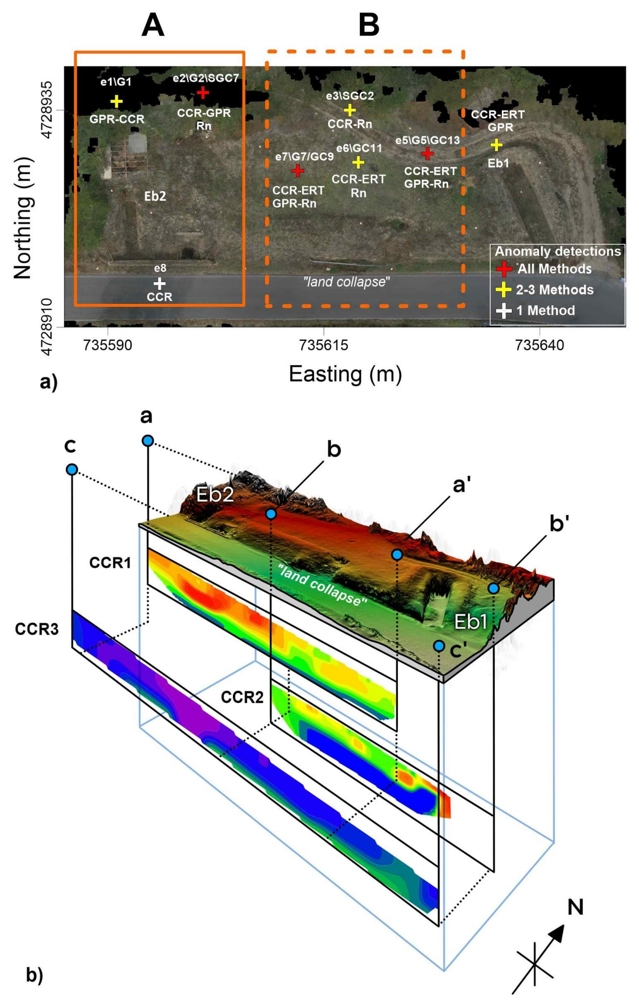
4.1. Geophysical and Geochemical Data Overlay

Figure 8 shows the comparison between the models obtained via ERT, CCR, and GPR techniques. The anomaly due to the Eb1 excavated chamber is clearly recognizable in all geophysical datasets. However, it differs in shape and depth depending on the adopted geophysical method. Meanwhile, the ERT provided a good result in terms of anomaly position and its roof and floor depth detection; the Eb1 CCR anomaly was not correctly reconstructed by the inversion algorithm due to the lack of survey data due to the presence of the metallic fence obstruction along the path. Two main differences were identified between the CCR and ERT output models. Owing to its higher shallow resolution, the ERT resistivity model highlighted the presence of an uppermost lower-resistive layer (ρ < 200 Ohm.m), approximately 1 m thick throughout the section, that was not imaged by CCR data. The western resistivity anomaly (e7) is suggested to have geometrical aspects similar to that of the adjacent anomalies e5 and e6 as compared with the CCR model, which does not precisely locate this anomaly. Note that the CCR dipoles have a minimum dimension of 5 m and thus are unable to depict the resistivity signature of the uppermost layer due to the inherent lower sensitivity at very shallow depth.
As for the e5 resistivity anomaly, the GPR profile showed continuous strong reflections, locating a small void between the roof chamber and the filling material. It also provided an accurate view of the chamber width, but not the floor position, even though the diffuse diffractions due to the chaotic filling material suggest a buried volume. Meanwhile, the ERT model showed a very similar result as the roof anomaly generated a resistive thin layer at a depth of approximately 1.5 m. Similar to GPR, the chamber shape was not recognizable, meaning that the host and fill materials had similar electric properties. Further, the uppermost resistivity variations highlighted by the ERT model in correspondence of the e5 anomaly probably affected the accurate imaging of this anomaly. Conversely, the CCR model is practically insensitive to this effect as no apparent resistivity data were measured for that portion of the ground. As a matter of fact, we could invert a simpler resistivity context (averaged top layer with a void inside) that was largely affected by the imposed starting model (⍴ ≃ 600 Ohm.m) in the uppermost portion of the model.
The e6 anomaly is practically undetected in the GPR radargrams because of the slight difference (less than 0.7 m) between the GPR2/GPR3 and CCR2 paths in that area. This confirms the dependence of our results on the precision in profile overlays when using high-resolution methods.
Figure 9 shows the comparison between the results obtained along the profiles CCR1 and GPR1 acquired on the small northwest-southeast oriented trail. The GPR1 radargram provides a clear image of the separated anomalies (G1, G2, and G3), which is probably due to the presence of partially filled voids.
Conversely, in the CCR model, the e2 anomaly is similar to G2, but it appears more confined in space and magnitude. The G3 anomaly shows some relation to the e3 CCR anomaly, which appears to be related to the G3 lateral extension. Such differences could be reasonably attributed to the change in survey direction and the presence of obstacles above the surface, which probably caused inaccurate positioning of the CCR anomalies along the profile with respect to the GPR line.
Figure 10 reports the Th/Rn ratio from stations that overlay the CCR2 profile. We found a good correlation between the high values measured in samples GC9 (A1), GC11 (A2), and GC13 (A3) and the three resistivity anomalies recovered by the CCR2 and ERT profiles (e7, e6, and e5, Figure 8) and confirmed by ERT and GPR datasets.
Analyzing the trends, we identify a peak with greater intensity (A1), a peak with a lower intensity (A2), and a peak of intermediate intensity (A3). We interpreted these anomalous peaks as due to possible differences in terms of (a) relative depth of the source, (b) gas concentration and accumulation in empty or partially filled cavities, and (c) sealed or partially sealed cavities, which could have generated them. Therefore, considering the very rapid decay rate of Th (a few seconds) as compared to the Rn (a few days), the A1 Th/Rn anomaly suggests a shallower gas source. Note that a high Th/Rn ratio often indicates a deeper gas source, in which a gas carrier, such as CO2, can move the isotope from deep underground up to the surface through an advective mechanism [21]. However, since we measured CO2 flux values close to zero, the presence of Rn and Th is certainly due to the local volcanic rocks instead of deep sources.
A similar scenario can be considered for the A3 sample where, however, the lower calculated Th/Rn ratio suggests a slightly deeper gas source compared to A1. Differently, the low value of the gas’s ratio recorded in the A2 sample can be addressed to a gas source with similar characteristics to the A1 and A2 ones but where the cavity is not completely sealed laterally, thus facilitating the gas dispersion through secondary chambers/corridors or fractures not mapped by our geophysical surveys.
These variations in the Th/Rn ratio appear to correlate local differences in terrain resistivity in which higher values could be interpreted as due to the response of a void space while relatively lower resistivity range could be attributed to partially filled voids. It is worth noting that terrain or cavity sealing status plays an important role in the gas accumulation and thus in its detectability from the surface. Furthermore, by assuming the same size and depth of the cavities, whether they are empty or partially filled if the conditions of lateral circulation of gas (through small tunnels, pipes, etc.) are met, the amount of gas that can accumulate in the cavity decreases and consequently, its measured concentration.
On this basis, we interpreted the e6 anomaly as a semi-closed cavity with lateral air exchange and a lower gas accumulation rate. Conversely, we considered e7 and e5 as belonging to a closed system, in which the differences in the Th/Rn ratio could be attributed to a small variation in the source depth.

4.2. Archeological Relevance of the Geophysical and Geochemical Results

The results obtained in this study evidenced the presence of buried features that can be interpreted as part of the assemblage of rock-cut chambers pertaining to burial structures. The recovered geometry of these chambers shows a very good correlation with those observed in neighboring sites (Figure 1), showing several adjacent chambers aligned at different levels (Figure 2) as already documented by [24].
A spatial pattern of such features emerged, articulating longitudinally between the two excavated tombs, Eb1 and Eb2, and between the modern road and the northern tuff plateau (Figure 11).
We suggest the recognition of at least two structures in such a pattern:
  • − The feature “A”, which includes the anomalies e1/G1, e2/G2/SGC7, and e8, which are spatially related to the excavated tomb Eb2.
  • − The feature “B”, which includes the anomalies e3/SGC2, e7/G7, GC9, e6/GC11, and e5/G5/GC13.
Note that the feature “B” does not show any electrical/EM signatures below the asphalt, although it is evident a land collapse along the road is visible in the DSM, which certainly suggests the presence of such a structure at least at the level of the roadside (Figure 11b). The unclear relationship between the e3 and G3 and between e2/G2 and G3 anomalies suggests caution in the interpretation of the “A” to “B” transition.
The resistivity anomalies e3 and e5/G5 are placed in an intermediate position between the feature “B” and the excavated tomb Eb1/G4. As a consequence, their belonging to one or the other might be questioned and can only be clarified through a focused archeological excavation.

5. Conclusions

This study presents the main results obtained through an integrated geophysical and geochemical survey at Vigna la Piazza necropolis aimed to find unidentified archeological burials.
The effectiveness of the integration between standard high-resolution geophysical methods applied to archaeological prospection was completed by the novelty of the joint use of Rn in soil measurements and CCR. The obtained results combining data from different methods showed good correlation and allowed us to build a map of possible archeological structures. The main limitations of the CCR method were found to be as follows: (i) rough resolution of targets, (ii) low resolution in the uppermost meter of soil, and (iii) possible mismatching in the target dimension and position due to uncertainty in the distribution of measurements along the survey line. Nevertheless, our experience in this study led us to consider the CCR method a very useful tool for a preliminary site investigation. Combining CCR and GPR grids, it is possible to obtain a deeper 3-D vision of buried archaeological structures, covering large areas in a relatively short time.
The determination of the Th/Rn ratio provided useful information to point out zones characterized by the presence of shallow empty or partially empty cavities. Since several necropolises and acropolises in central Italy were constructed with and within tuff materials, the Rn in soil measurements can be successfully applied. Finally, this paper suggests that Rn and CCR methods could be considered reliable tools for the preliminary investigation of such archaeological targets in a similar geological context, and the results will provide archaeologists with guidance on future archeological excavations.

Author Contributions

V.S.: Conceptualization, data curation, and writing—original draft preparation; V.M. and F.F.: investigation, formal analysis, visualization, and writing—review and editing; M.M. and M.F.M.: supervision, validation, and writing—review and editing; A.G. and N.V.: data acquisition, methodology, and writing—original draft preparation; F.G., R.C., and L.M.: investigation; S.U.: investigation, data curation, and writing—original draft preparation. All authors have read and agreed to the published version of the manuscript.

Funding

This research received no external funding.

Institutional Review Board Statement

Not applicable.

Informed Consent Statement

Written informed consent has been obtained from the patient(s) to publish this paper if applicable.

Data Availability Statement

The data presented in this study are openly available in repository FigShare at doi:10.6084/m9.figshare.15101835.

Acknowledgments

This work has been produced under the signed Research Agreement between the INGV and the Soprintendenza per i Beni Archeologici dell’Etruria Meridionale, in 2017. We are grateful to Maria Letizia Arancio, Director at Soprintendenza per i Beni Archeologici dell’Etruria Meridionale, for allowing us to access and work at Vigna La Piazza site and for fruitful discussion on the archaeological setting of Grotte di Castro. Thanks to Piero Camilli, Mayor of Grotte di Castro. We also thank Alessandra Sciarra, for supporting us in the geochemical data interpretation.

Conflicts of Interest

The authors declare that they have no known competing financial interests or personal relationships that could have appeared to influence the work reported in this paper.

References

  1. Pellegrini, E.; Leotta, M.C.; Pacetti, M.S.; Rafanelli, S.; Schiappelli, A.; Severi, E.; Buchicchio, F.T.F.Z.; Abbadessa, A.; Martino, C.; Occhiogrosso, F.; et al. Bolsena e la sponda occidentale della Val di Lago: Un aggiornamento. Mélanges École Française Rome Antiq. 2011, 123, 13–105. [Google Scholar] [CrossRef]
  2. Wynn, J.C. A review of geophysical methods used in archaeology. Geoarchaeology 1986, 1, 245–257. [Google Scholar] [CrossRef]
  3. Gaffney, C. Detecting trends in the prediction of the buried past: A review of geophysical techniques in archaeology. Archaeometry 2008, 50, 313–336. [Google Scholar] [CrossRef]
  4. Orlando, L.; Piro, S.; Versino, L. Location of sub-surface geoelectric anomalies for archaeological work: A comparison between experimental arrays and interpretation using numerical methods. Geoexploration 1987, 24, 227–237. [Google Scholar] [CrossRef]
  5. Lapenna, V. Resilient and sustainable cities of tomorrow: The role of applied geophysics. Boll. Geofis. Teor. Appl. 2017, 58, 237–251. [Google Scholar]
  6. Brizzolari, E.; Ermolli, F.; Orlando, L.; Piro, S.; Versino, L. Integrated geophysical methods in archaeological surveys. J. Appl. Geophys. 1992, 29, 47–55. [Google Scholar] [CrossRef]
  7. Smriglio, F.; Papale, E.; Verga, F.; Piro, S. Noninvasive geophysical integrated survey at Madonna del Giglio (Sabine necropolis, Magliano Sabina, Latium, Central Italy). Archaeol. Anthropol. Sci. 2020, 12, 79. [Google Scholar] [CrossRef]
  8. Porcelli, F.; Sambuelli, L.; Comina, C.; Spanò, A.; Lingua, A.; Calantropio, A.; Catanzariti, G.; Chiabrando, F.; Fischanger, F.; Maschio, P.; et al. Integrated Geophysics and Geomatics Surveys in the Valley of the Kings. Sensors 2020, 20, 1552. [Google Scholar] [CrossRef] [Green Version]
  9. El Aguizy, O.O.; Gobashy, M.M.; Metwally, A.; Aoliman, K.S.; Nader, E.L. The discovery of the tomb of the Great Army General Iwrhya: A quasi 3D Electrical Resistivity Tomography (ERT), Saqqara, Giza, Egypt. Contrib. Geophys. 2020, 50, 425–446. [Google Scholar]
  10. Cozzolino, M.; Baković, M.; Borovinić, N.; Galli, G.; Gentile, V.; Jabučanin, M.; Mauriello, P.; Merola, P.; Živanović, M. The Contribution of Geophysics to the Knowledge of the Hidden Archaeological Heritage of Montenegro. Geosciences 2020, 10, 187. [Google Scholar] [CrossRef]
  11. Di Mauro, D.; Alfonsi, L.; Sapia, V.; Urbini, S. A neighborhood revealed by geophysical prospection: An example of urbanization at the Phoenician–Punic settlement of Mozia (western Sicily, Italy). J. Appl. Geophys. 2014, 104, 114–120. [Google Scholar] [CrossRef]
  12. Dick, H.C.; Pringle, J.K.; Wisniewski, K.D.; Goodwin, J.; Van Der Putten, R.; Evans, G.T.; Francis, J.D.; Casella, P.; Hansen, J.D. Determining geophysical responses from burials in graveyards and cemeteries. Geophysics 2017, 82, B245–B255. [Google Scholar] [CrossRef] [Green Version]
  13. Bottacchi, M.C.; Colonna, T.; Mantovani, F.; Medri, M. Application of the OhmMapper resistivity-meter to detect the theatre of Sentinum Roman town by using 3D resistivity model. ArcheoSciences Rev. Archéométrie 2009, 33, 267–269. [Google Scholar] [CrossRef] [Green Version]
  14. Sapia, V.; Florindo, F.; Marchetti, M.; Di Nezza, M. Fast geophysical prospection to map the archaeological site of Cocciano: Preliminary results. Ann. Geophys. 2017, 60. [Google Scholar] [CrossRef] [Green Version]
  15. Sapia, V.; Baccheschi, P.; Villani, F.; Taroni, M.; Marchetti, M. Multidisciplinary geophysical approach to map a disposal site: The Ponza island case study. J. Appl. Geophys. 2017, 138, 264–274. [Google Scholar] [CrossRef]
  16. Haslam, R.; Tibbett, M. Sampling and analyzing metals in soils for archaeological prospection: A critique. Geoarchaeology 2004, 19, 731–751. [Google Scholar] [CrossRef]
  17. Linderholm, J. Soil chemical surveying: A path to a deeper understanding of prehistoric sites and societies in Sweden. Geoarchaeology 2007, 22, 417–438. [Google Scholar] [CrossRef]
  18. Entwistle, J.A.; Abrahams, P.W.; Dodgshon, R.A. The geoarchaeological significance and spatial variability of a range of physical and chemical soil properties from a former habitation site, Isle of Skye. J. Archaeol. Sci. 2000, 27, 287–303. [Google Scholar] [CrossRef]
  19. Parnell, J.J.; Terry, R.E.; Nelson, Z. Soil chemical analysis applied as an interpretive tool for ancient human activities at Piedras Negras, Guatemala. J. Archaeol. Sci. 2002, 29, 379–404. [Google Scholar] [CrossRef]
  20. Middleton, W.D. Identifying chemical activity residues on prehistoric house floors: A methodology and rationale for multi-elemental characterization of mild acid extract of anthropogenic sediments. Archaeometry 2004, 46, 47–65. [Google Scholar] [CrossRef]
  21. Lucchetti, C. Valutazione dell’Influenza di Cavità Sotterranee e Campi di Fratturazione Sulle Concentrazioni di Radon e Thoron nel Suolo in Aree Idrotermali e Peri-Vulcaniche della Regione Lazio. Ph.D. Thesis, Università Degli Studi Roma Tre, Rome, Italy, 2014. [Google Scholar]
  22. Oonk, S.; Slomp, C.P.; Huisman, D.J. Geochemistry as an aid in archaeological prospection and site interpretation: Current issues and research directions. Archaeol. Prospect. 2009, 16, 35–51. [Google Scholar] [CrossRef]
  23. Manca, F.; Viaroli, S.; Mazza, R. Hydrogeology of the Sabatini Volcanic District (Central Italy). J. Maps 2017, 13, 252–259. [Google Scholar] [CrossRef]
  24. Tamburini, P. Etruschi e Romani nel Territorio di Grotte di Castro. In Grotte di Castro: Il Territorio, Il Paese, Il Museo; Città di Bolsena: Bolsena, Italy, 2007; pp. 13–65. [Google Scholar]
  25. Moffat, I. Isotope Geochemistry in Archaeology. In Encyclopedia of Global Archaeology; Springer: New York, NY, USA, 2014; pp. 4106–4110. [Google Scholar]
  26. Pelagotti, A.; Uccheddu, F.; Nex, F.; Remondino, F.; Chisari, L. Automatic graves’ orientation detection: A tool for spatial archeology. In Proceedings of the 8th International Symposium on Image and Signal Processing and Analysis, Trieste, Italy, 4–6 September 2013; pp. 582–587. [Google Scholar]
  27. Yuan, B.; Liu, S.; Lu, G. An integrated geophysical and archaeological investigation of the emperor Qin Shi Huang mausoleum. J. Environ. Eng. Geophys. 2006, 11, 73–81. [Google Scholar] [CrossRef]
  28. Kovler, K. Radioactive materials. In Toxicity of Building Materials; Pacheco-Torgal, F., Jalali, S., Fucic, A., Eds.; Elsevier: Amsterdam, The Netherlands, 2012. [Google Scholar]
  29. Gundersen, L.C.; Wanty, R.B. Field Studies of Radon in Rocks, Soils, and Water, 1st ed.; United States Geological Survey: Alexandria, VA, USA, 1991. [Google Scholar]
  30. Urbini, S.; Cafarella, L.; Marchetti, M.; Chiarucci, P.; Bonini, D. Fast geophysical prospecting applied to archaeology: Results at Villa ai Cavallacci (Albano Laziale, Rome) site. Ann. Geophys. 2007, 50, 291–299. [Google Scholar]
  31. ISPRA. La Geologia di Roma: Dal Centro Storico alla Periferia; ISPRA: Rome, Italy, 2008; Volume 80. [Google Scholar]
  32. Acocella, V.; Palladino, D.M.; Cioni, R.; Russo, P.; Simei, S. Caldera structure, amount of collapse, and erupted volumes: The case of the Bolsena caldera, Italy. Geol. Soc. Am. Bull. 2012, 124, 1562–1576. [Google Scholar] [CrossRef]
  33. Peccerillo, A. Cenozoic Volcanism in the Tyrrhenian Sea Region, 1st ed.; Advances in Volcanology; Springer: Berlin/Heidelberg, Germany, 2017. [Google Scholar]
  34. Salamone, F. La Civita di Grotte di Castro. Carta Archeologica. 2011. Available online: https://www.academia.edu/12960384/La_Civita_di_Grotte_di_Castro_Carta_archeologica (accessed on 25 July 2021).
  35. Groom, D. Common misconceptions about capacitively-coupled resistivity (CCR), what it is and how it works. In 21st Symposium on the Application of Geophysics to Engineering and Environmental Problems; European Association of Geoscientists & Engineers: Houten, The Netherlands, 2008; p. 177. [Google Scholar]
  36. Timofeev, V.M. The Employment of Capacitively-Coupled Sensors in Engineering and Geological Studies. Ph.D. Thesis, University of Moscow, Moscow, Russia, 1974. [Google Scholar]
  37. Kuras, O.; Beamish, D.; Meldrum, P.I.; Ogilvy, R.D. Fundamentals of the capacitive resistivity technique. Geophysics 2006, 71, G135–G152. [Google Scholar] [CrossRef] [Green Version]
  38. Loke, M.H.; Barker, R. Rapid least-squares inversion of apparent resistivity pseudo-sections using a quasi-Newton method. Geophys. Prospect. 1996, 44, 131–152. [Google Scholar] [CrossRef]
  39. Annan, A.P.; Davis, J.L. Radar range analysis for geological materials. Geol. Surv. Can. 1977, 77, 117–124. [Google Scholar]
  40. Grimm, R.E.; Heggy, E.; Clifford, S.; Dinwiddie, C.; McGinnis, R.; Farrell, D. Absorption and scattering in ground-penetrating radar: Analysis of the Bishop Tuff. J. Geophys. Res. Planet 2006, 111, E06. [Google Scholar] [CrossRef] [Green Version]
  41. Heggy, E.; Clifford, S.M.; Grimm, R.E.; Dinwiddie, C.L.; Wyrick, D.Y.; Hill, B.E. Ground-penetrating radar sounding in mafic lava flows: Assessing attenuation and scattering losses in Mars-analog volcanic terrains. J. Geophys. Res. Planet 2006, 111, E6. [Google Scholar] [CrossRef] [Green Version]
  42. Robinson, D.A.; Friedman, S.P. A method for measuring the solid particle permittivity or electrical conductivity of rocks, sediments, and granular materials. J. Geophys. Res. Solid Earth 2003, 108, B2. [Google Scholar] [CrossRef] [Green Version]
  43. Ghezzi, A.; Schettino, A.; Pierantoni, P.P.; Conyers, L.; Tassi, L.; Vigliotti, L.; Vigliotti, L.; Schettino, E.; Melfi, M.; Gorrini, A.E.; et al. Reconstruction of a Segment of the UNESCO World Heritage Hadrian’s Villa Tunnel Network by Integrated GPR, Magnetic–Paleomagnetic, and Electric Resistivity Prospections. Remote Sens. 2019, 11, 1739. [Google Scholar] [CrossRef] [Green Version]
  44. Voltattorni, N.; Quattrocchi, F.; Gasparini, A.; Sciarra, A. Soil gas degassing during the 2009 L’Aquila earthquake: Study of the seismotectonic and fluid geochemistry relation. Ital. J. Geosci. 2012, 131, 440–447. [Google Scholar]
  45. Sinclair, A.J. A fundamental approach to threshold estimation in exploration geochemistry: Probability plots revisited. J. Geochem. Explor. 1991, 41, 1–22. [Google Scholar] [CrossRef]
  46. Harris, J.R.; Viljoen, D.W.; Rencz, A.N. Integration and visualization of geoscience data. In Remote Sensing for the Earth Sciences; John Wiley & Sons: Hoboken, NJ, USA, 1999; Volume 3, pp. 307–354. [Google Scholar]
  47. Oldenborger, G.A.; LeBlanc, A.M. Geophysical characterization of permafrost terrain at Iqaluit International Airport, Nunavut. J. Appl. Geophys. 2015, 123, 36–49. [Google Scholar] [CrossRef]
  48. McNeill, J.D. Electromagnetic Terrain Conductivity Measurement at Low Induction Numbers; Geonics Limited Technical Note, TN-6; Geonics Limited: Mississauga, ON, Canada, 1980; pp. 6–15. [Google Scholar]
  49. Oldenborger, G.A.; LeBlanc, A.M. Capacitive resistivity inversion using effective dipole lengths for line antennas. J. Appl. Geophys. 2013, 98, 229–236. [Google Scholar] [CrossRef]
Figure 1. Geological and archaeological map.
Applsci 11 07875 g001
Figure 2. Schematic tomb structure. (a) Plan and (b) cross-section view of one of the rock-cut chamber tombs in Vigna la Piazza (VLP7) showing the typical burial morphology. Adapted from [24].
Applsci 11 07875 g002
Figure 3. Location map of the geophysical and geochemical surveys. Study area with the location of the geophysical and the geochemical surveys. Insets show (a) CCR and (b) GPR survey operations, wherein the solid-yellow dots indicate the sampled geochemical data, the light-blue solid lines indicate the CCR profiles, while the solid purple and green lines show the GPR and the ERT profiles, respectively.
Applsci 11 07875 g003
Figure 4. CCR resistivity sections. CCR inversion results of (a) profile a-a’, RMS 5.9% after six iterations (CCR1 in Figure 3); (b) profile b-b’, root mean square (rms) 5.4% after five iterations (CCR2 in Figure 3), and (c) profile c-c’, RMS 3.8% after five iterations (CCR3 in Figure 3). The solid black lines indicate the interpreted interface between units A and B. The topographies of the profiles were extracted via a high-resolution digital surface model (DSM). Recovered CCR anomalies are labeled with letters from e1 to e8.
Applsci 11 07875 g004
Figure 5. ERT resistivity section. Electrical resistivity tomography (ERT) recovered resistivity model. Root mean square (rms) 2.5% after six iterations.
Applsci 11 07875 g005
Figure 6. GPR radargrams. GPR radargrams obtained in the Vigna la Piazza Necropolis along (a) line b-b’ (GPR2 profile partially coincident with CCR2 line in Figure 3), (b) line c-c’ (GPR3 profile partially coincident with CCR2 line in Figure 3), and (c) line a-a’ (GPR1 profile partially coincident with CCR1 line in Figure 3). The dashed white lines mark the GPR anomalies associated with the presence of excavated (Eb1) and partially filled burials. Recovered GPR anomalies are labeled with capital letters from G1 to G7.
Applsci 11 07875 g006
Figure 7. Rn and Th maps. Geochemical maps for the measured (a) Th and Rn concentrations: Red and yellow squares show areas of very high and high Rn concentrations, while green and white ones represent low and very low concentrations. Th concentrations are classified into four classes represented by different light-blue circle dimensions; (b) Th/Rn ratios: Red and yellow circles indicate areas of very high and high ratios while light-blue and blue circles represent low and very low ratio values.
Applsci 11 07875 g007
Figure 8. Geophysical data comparison. Comparison between all sets of output geophysical models recovered over a coincident line (CCR1, GPR2, GPR3, and ERT profiles in Figure 3). (a) ERT model and (b) image of the already excavated tomb Eb1. (c) CCR1 resistivity model. (d) GPR3 and GPR2 radargrams, wherein the dashed white lines mark the GPR anomalies attributed to the presence of the excavated (Eb1) and partially filled burials. The CCR and ERT profile topographies were extracted from a high-resolution digital surface model.
Applsci 11 07875 g008
Figure 9. Geophysical data comparison. Comparison between (a) CCR2 resistivity model and (b) GPR1 radargram along the northwest-southeast oriented trail. Dashed white lines mark GPR anomalies attributed to the presence of partially filled voids.
Applsci 11 07875 g009
Figure 10. Geophysical and geochemical data comparison. Rn/Th values overlaid on the CCR1 profile (b-b’, see Figure 3 for profile location). Yellow dots in the satellite image locate the geochemical measurements selected to develop the Rn/Th ratio profile.
Applsci 11 07875 g010
Figure 11. Location map of the recovered anomalies. (a) Orthophoto of the survey area with the location of the entire set of recovered geophysical and geochemical anomalies. Solid-red crosses indicate the position of the anomalies as mapped from all applied methods, while yellow and white crosses locate the anomalies as recovered from two/three and one single method, respectively. Solid and dashed-orange rectangles show the interpreted burial structures organization. (b) DSM derived by Structure-from-Motion photogrammetry superimposed on the CCR profiles in a 3-D perspective.
Applsci 11 07875 g011
Publisher’s Note: MDPI stays neutral with regard to jurisdictional claims in published maps and institutional affiliations.

