1. Introduction
Programs to simulate a variety of mechanisms were initially developed to solve mathematical equations involved in the interconnection among elements of such mechanisms. The solving of systems of non-linear algebraic equations (or algebraic–differential equations in the case of dynamics) was a constant “burden” every time a mechanism had to be analyzed. General-purpose multibody dynamics programs subsequently emerged with the same target as general-purpose finite element programs. Among the softwares available at the time, the following general-purpose multibody dynamics programs were prominent: ADAMS [
1,
2], AUTOLEV [
3], COMPAMM [
4], DADS [
5], DYMAC [
6], and MESA [
7]. This paper focuses on programs intended for mechanism simulations related to education, and few of them have any didactic capacity. It is challenging to find references in the literature where general-purpose programs are used for teaching. Some specific cases can be found, such as the Virtual Lab based on ADAMS presented in [
8]. The authors claimed, however, that the exercises to be solved by students need to be carefully selected due to the complexity of the program. On the contrary, they remarked the advantage of employing a program that is commonly used in the industry so that students can learn it in college.
Another group of more specific programs for the analysis and synthesis of mechanisms was developed in the context of mechanisms and machine theory (MMT). The following are noteworthy: KINSYN [
9], LINCAGES [
10], and RECSYN [
11]. University lecturers in machines and mechanisms have participated in the development of these programs, because of which they focus on a didactic approach. Recent softwares in this group are MechDev [
12] and WinMecC [
13,
14], both dedicated to the analysis and synthesis of planar mechanisms. The most remarkable characteristic of WinMecC is its dimensional synthesis module based on evolutionary algorithms. MechDev has a special architecture based on plug-ins, including an algorithm that combines analytical with numerical computation. Another powerful program similar to them is Working Model 2D [
15], which is capable of modeling mechanisms in an interactive way.
Dynamic geometric environments (DGEs) are software tools that are being commonly used nowadays to teach MMT. They allow for the building of parametrized geometric entities. GeoGebra [
16] is a representative DGE. Mathematical libraries that can be used to support the teaching of many subjects related to mechanism and machine science are another type of technological tools. For example, the graphical programming environment Simulink of MATLAB is a good choice for implementing and solving the dynamics of the mathematical models of mechanical systems [
17]. The MATLAB framework has proven to be useful for the development of active teaching–learning methodologies, such as the one designed to teach kinematic and dynamic analyses of 3D multibody systems proposed in [
18]. Finally, there are some cases in which CAD systems have been used to simulate mechanisms for teaching. However, this does not appear to be the most adequate option as they are not specific programs for mechanisms, are usually expensive, and do not focus on didactic approaches.
The software presented in this paper (GIM), the initial steps of which were introduced in [
19], is a general-purpose software that can handle planar and spatial systems of any number of degrees of freedom. It was developed by the COMPMECH research group of the Department of Mechanical Engineering of the University of the Basque Country UPV/EHU in Spain. It is designed for teaching and learning activities related to important subjects in mechanical engineering, such as applied mechanics, mechanism and machine theory, computational kinematics and dynamics, mechanical design, and robotics. GIM has also been used as a tool for the development of several doctoral theses, and their results have served as important feedback to develop and improve its computational modules.
2. Capabilities and Potential of GIM
One of the aims of using GIM is to help students better understand the theoretical concepts explained in lectures in class, and to motivate them to work independently with the software to develop their skills on it. The software is available for free.
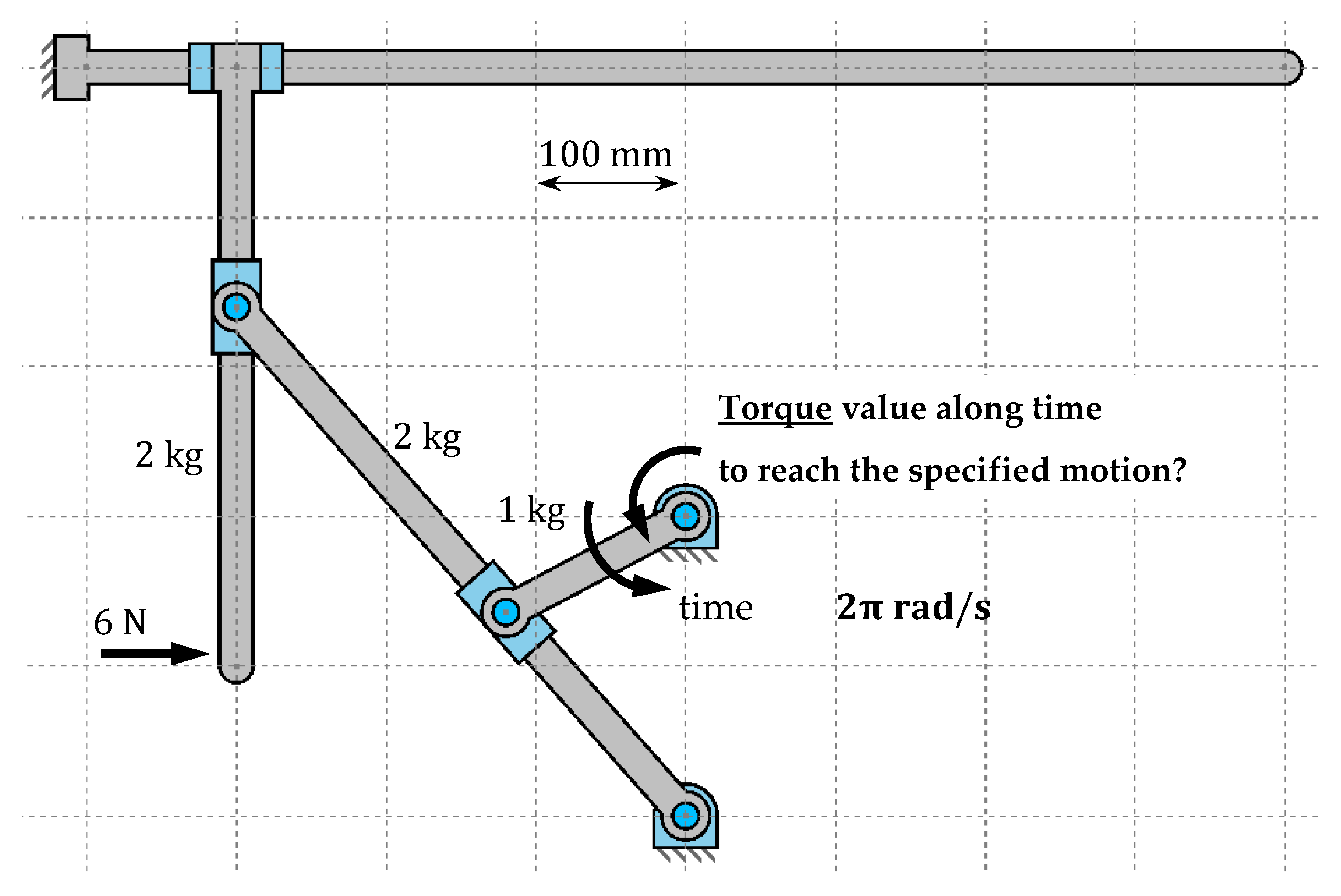
This section provides a general idea to the reader of the tools provided by GIM related to the learning process. A planar example is first developed. The case study chosen is the quick return mechanism, and is posed in the same way that it would be to students. The goal is to obtain the value of the actuating torque required to achieve a specified motion when some resisting loads are applied as shown in
Figure 1.
To solve this exercise, students have to follow basic steps:
Create the geometrical model of the mechanism.
Define the function of input motion and solve the kinematics.
Define existing resistant loads and solve the inverse dynamics (kinetostatic problem).
Since simply an example is not enough to show the potential of this software and all options that the students can exploit to improve their learning skills, additional aspects are explained.
2.1. Geometry Module—Case Study
A kinematic sketch is a geometrical model of the mechanism in which ideal joints are considered and elements are modeled as perfectly rigid bodies. The student can build the geometrical model to make a kinematics or dynamics simulation simply and quickly. A trained user can have any model ready for simulation in a few minutes.
For analysis, the mechanism is defined directly in an assembled position, but not necessarily with empirical dimensions. The first step consists of defining the points of interest of the mechanical system, called nodes. To do this, the students can directly type the coordinates of the nodes or set their positions using the mouse pointer. In the second step, using these nodes, elements of the mechanism are built. The user simply selects the nodes belonging to the same element. Finally, the kinematic joints between elements are set from a list.
Even in the process of geometrical definition, students can compare the results with their knowledge, because each time a geometrical change is made, the program computes the number of degrees of freedom and the number of redundant constraints of the model in its given state.
Once the topology of the mechanism has been defined, the user can still modify the position of any node and orientation of any joint, or—what constitutes a more practical capability—can edit such values of the geometrical constraints as lengths of elements or angles between them. This is useful because the empirical geometrical data of a mechanism is often given by the sizes of elements and certain positional constraints, but does not include the coordinates of the moving nodes.
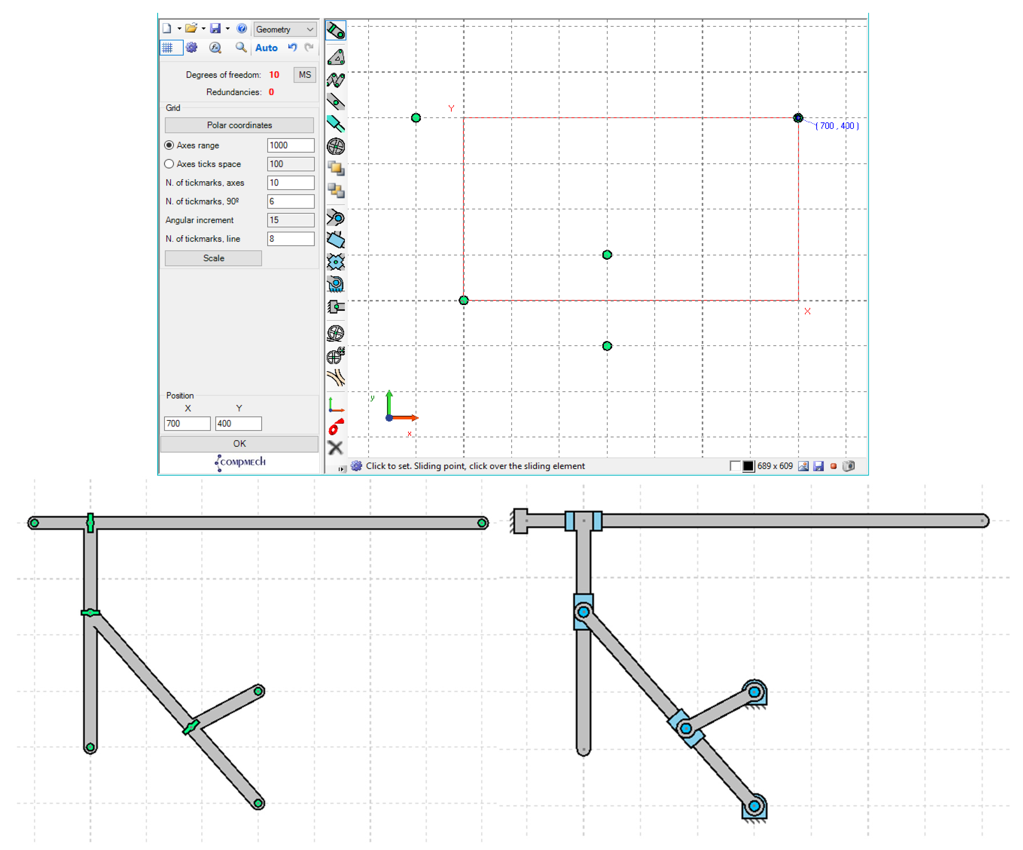
Figure 2 shows the process of generating the geometrical model of the Quick Return mechanism, which is used as an example to illustrate the teaching/self-learning capabilities of the program. This paper is not intended to be a user manual, and accordingly, practical instructions are not provided. The images of the software provided here should be sufficient for the reader to understand the main idea of GIM.
Geometry Module–Additional Considerations
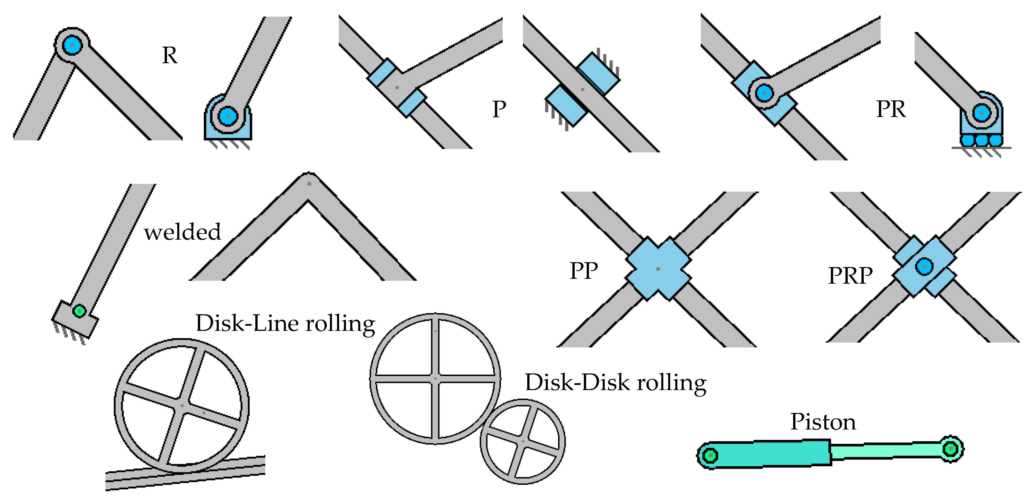
The GIM is a general-purpose software that can to deal with planar and spatial systems of any number of degrees of freedom. This is why the geometry module implements a wide collection of kinematic joints including all the most commonly used ones in practice (
Figure 3 and
Figure 4).
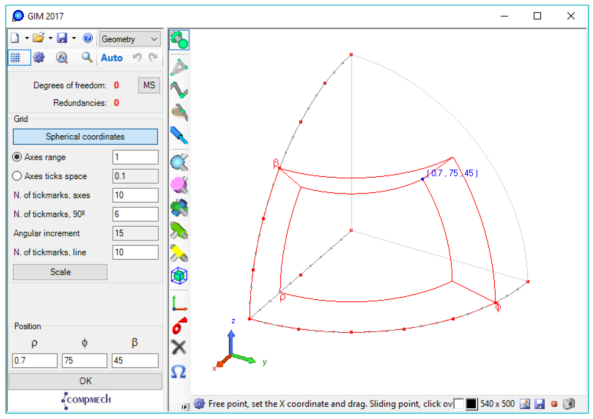
Some of them require the definition of additional geometric information—for example, the orientation of axes of the joint for spatial revolution. In these cases, once more, the student can use the keyboard or the mouse (with or without a grid option). Any joint type can be set as a fixed joint by connecting elements with a fixed frame. Moreover, the most convenient system of coordinates (Cartesian or polar) can be used in the geometric function (
Figure 5). The spatial joints and links are modeled as easily as the planar ones.
2.2. Kinematics Module—Case Study
The three main kinematic problems, i.e., those of position, velocity, and acceleration, can be solved in GIM. For this, the student needs to define as many actuators as the number of degrees of freedom of the mechanism. Each actuator is established as a motion function that specifies the value of its position variable, and the first and second derivatives along time. The most common types of actuators (fixed rotations, relative rotations, pistons, and sliders) as well as the most common types of motion functions (constant velocity or acceleration, polynomial, sinusoidal) are provided. The multibody approach based on natural coordinates is implemented to obtain the primary results: the simulation of motion of the mechanism (trajectories of all nodes, and velocities and accelerations at all nodes in each position).
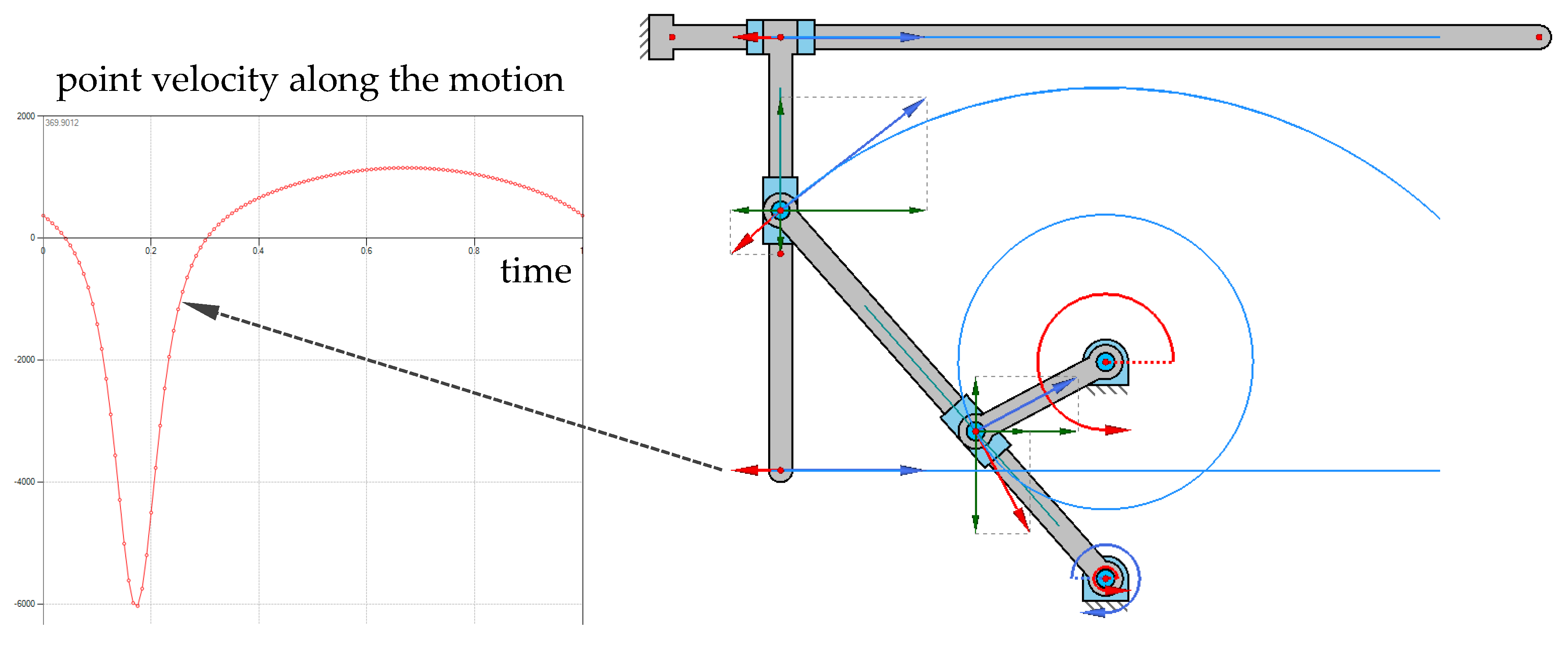
As shown in
Figure 6, all results can be graphically plotted along with the mechanism at any position, which makes it possible to visually analyze their evolution during motion. It also becomes possible to evaluate the variation of any parameter along the time tracing the corresponding function.
Using this computation module, apart from having at hand the numerical results of the proposed problem (as a mechanism calculator), students can corroborate the relevant theoretical concepts studied during lectures. Some examples are shown in
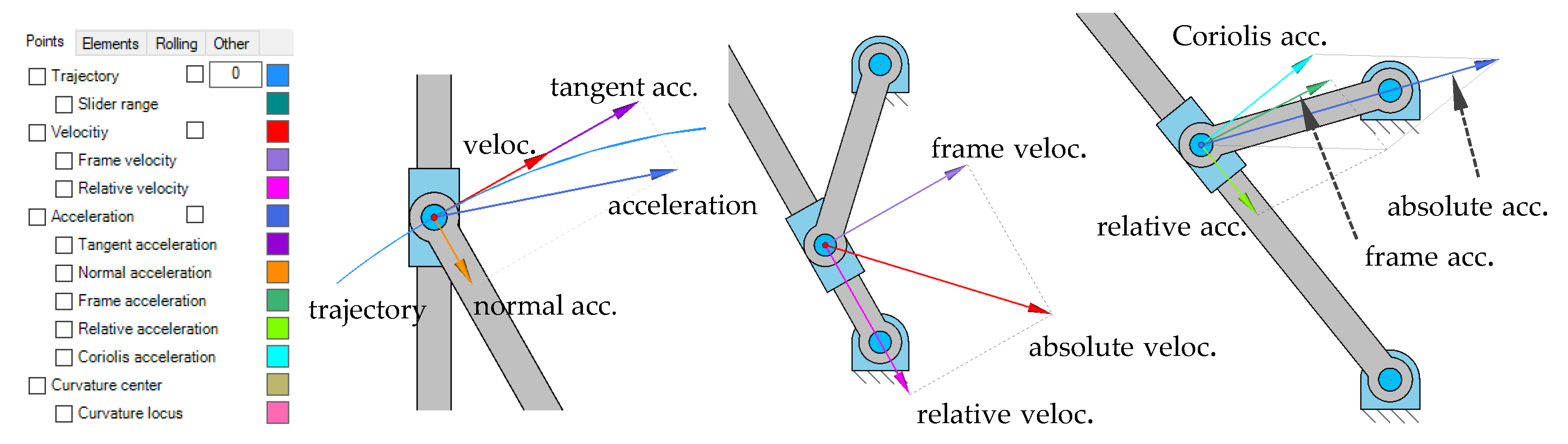
Figure 7:
They can observe how the velocity is always tangential to the trajectory while watching the motion of the mechanism.
They verify the decomposition of acceleration into a tangential component and a normal component pointing to the center of curvature of the trajectory. The ways in which intrinsic components are related to changes in the module and direction of the velocity vector can be graphically verified.
In the context of relative motion, they realize how this decomposition is made in relative and frame (and the Coriolis acceleration) components. They can verify that the Coriolis acceleration is always perpendicular to relative velocity.
Once the analysis has been concluded, the student can modify any kinematic or geometric parameter to see how this affects the results, which are recomputed in real time.
Kinematics Module—Additional Considerations
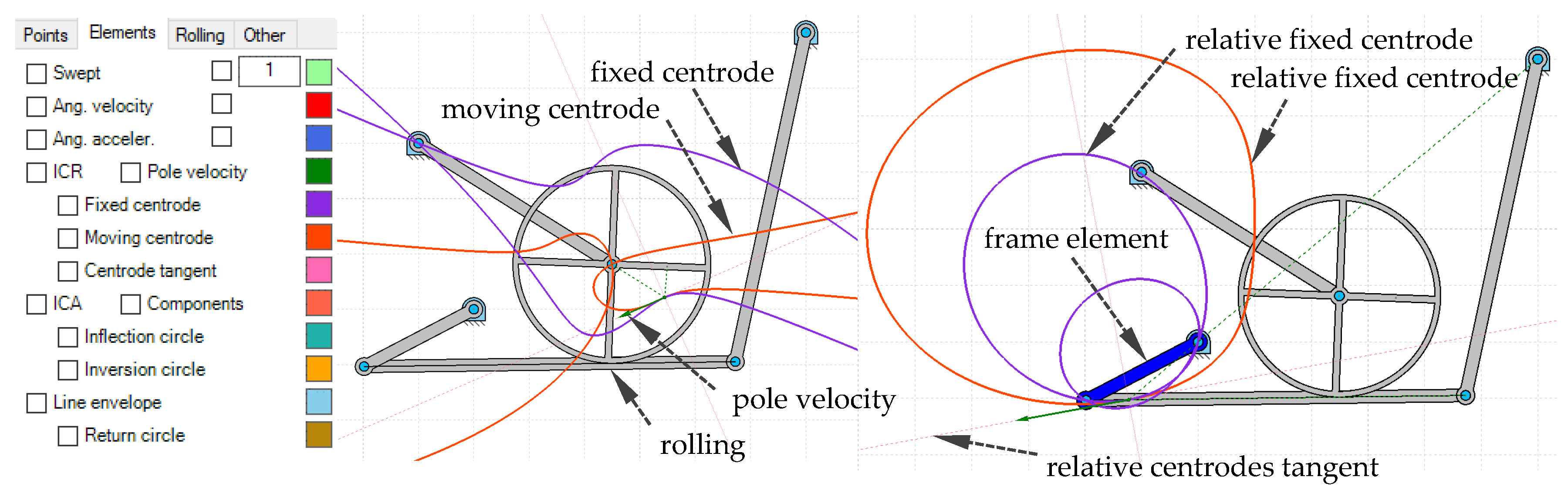
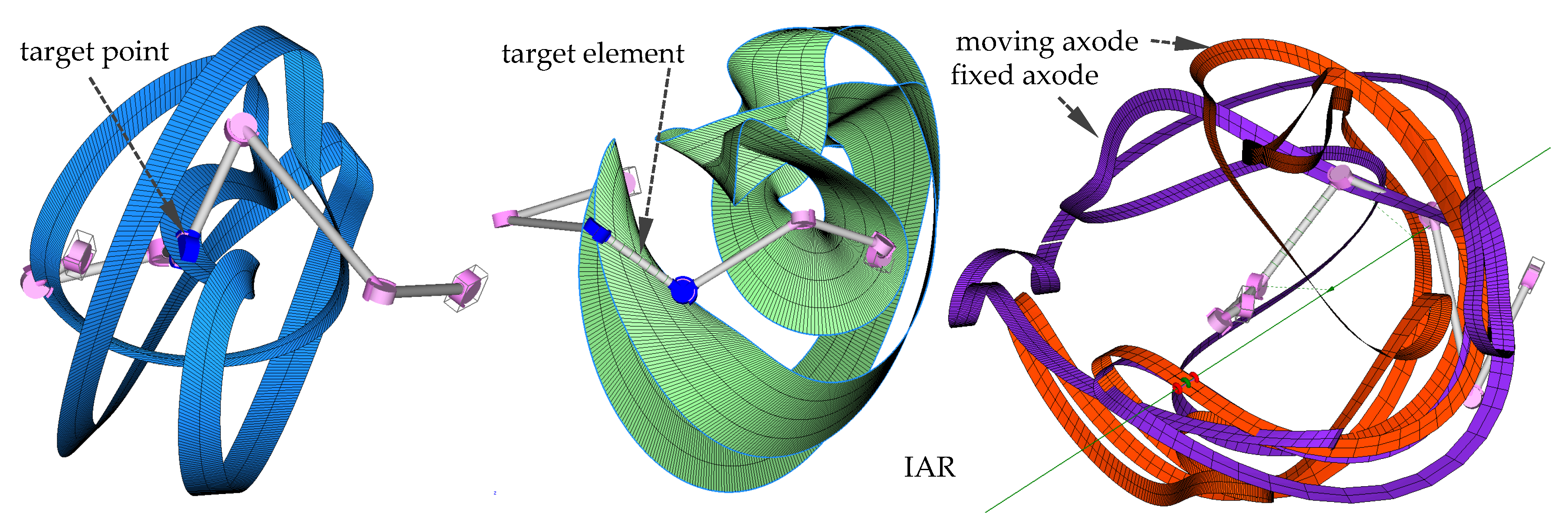
Apart from the main results, additional derived results are provided, such as the centers of curvature of the points, instantaneous centers of rotation of the elements, and fixed and moving centrodes. In addition, all results can be computed in terms of absolute motion or that relative to any moving element. Some of these additional capacities are shown in
Figure 8,
Figure 9,
Figure 10 and
Figure 11.
2.3. Dynamics Module–Case Study
Dynamic problems consider simultaneously motion and forces. GIM can solve two main types of dynamics problems, i.e., problems in inverse dynamics (kinetostatic problem) and direct dynamics. If all actuators are controlled in terms of position, velocity, and acceleration, as in the kinematics module, the motion of the mechanism is defined and can be computed independently from the existing forces. The unknowns of this problem are the values of the driving loads required to achieve such motion (considering resistant applied loads), and are computed by means of a kinetostatic approach. On the contrary, when all applied load values are known, the resulting motion is dependent on such values, i.e., the motion cannot be computed using a purely kinematic approach, and the direct dynamics problem has to be simulated.
Apart from driving loads (known values in direct dynamics but unknowns in inverse dynamics), the student can define as many external resistant loads as desired. The available loads are punctual as well as linearly distributed forces and torques. In this module, to compute inertial loads, the properties of mass of each element need to be specified. The default values of the center of gravity and moment of inertia are automatically computed depending on the shape of the element, but because this shape is sometimes just a kinematic sketch (the real element may have a different shape), these defaults can be substituted by custom values. Elemental weights are also considered if a value of gravitational acceleration is defined.
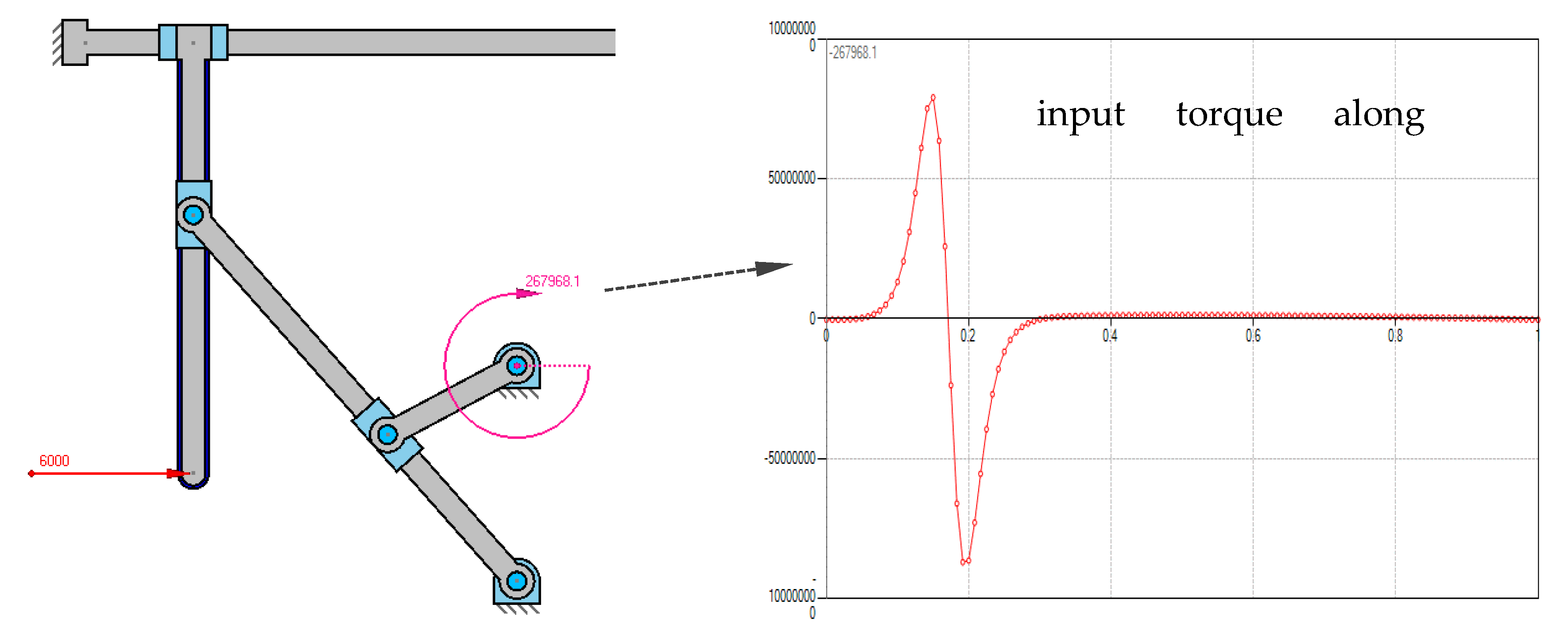
Figure 12 shows the proposed case study, and the value of the torque required over time to achieve a specific constant rotational velocity in the actuator under certain external loads.
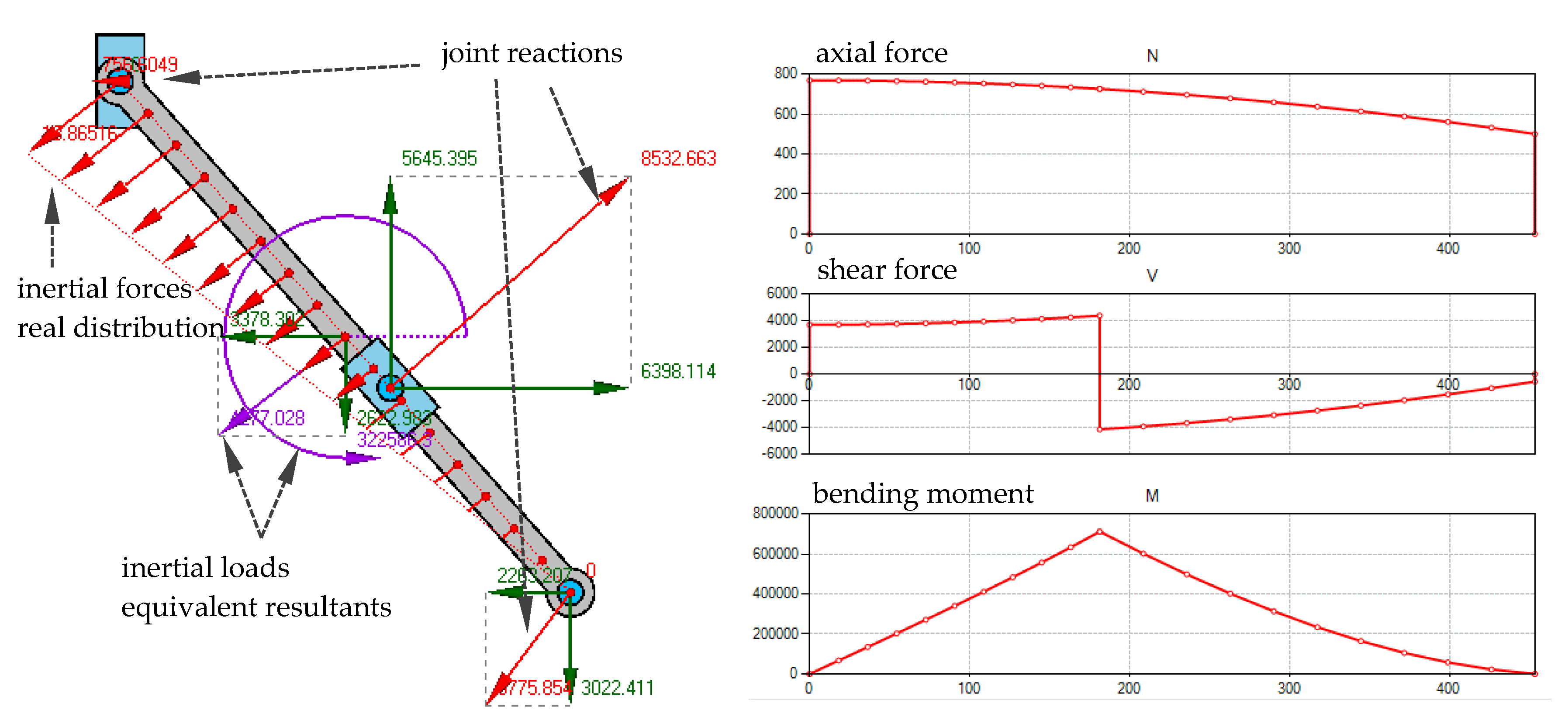
A number of additional results can be visualized apart from the above. In any dynamics problem, if the mechanism is non-redundant, a complete analysis of the force of the mechanical system is performed to compute the reaction forces and torques at the joints between elements. In addition, for linear elements, a diagram of internal efforts can be computed. As shown in
Figure 13, the real distribution of weight and inertial forces along the element are considered. This force analysis is conducted for each position of the simulation, and thus the evolution of any of these results can be represented along the motion.
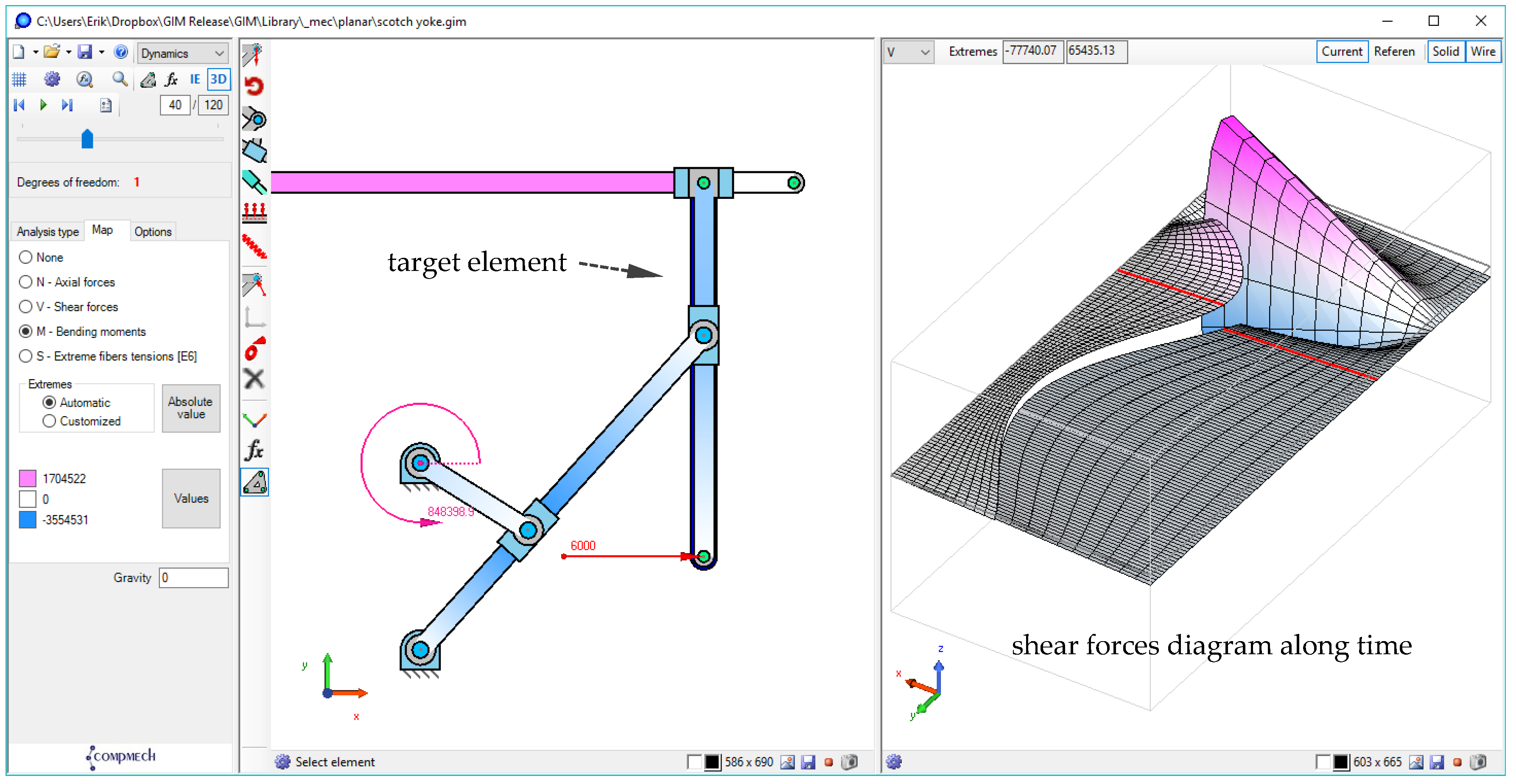
The student has the option of visualizing the values of any internal effort as a color map for the entire mechanical system at a position. Any internal effort diagram of an element can be also traced along time (motion), as shown in
Figure 14.
Using the tools provided in the computation module, the students can check/verify in a very clear way some of the concepts imparted to them theoretically, such as the following:
Although they had the same kinematics, the inertial properties of elements affected their dynamical results.
Discontinuities in the internal efforts’ diagrams are related to the existence of punctual loads at the relevant points.
The type of reaction load depends on joint type, but the action–reaction principle is always verified.
Other characteristics, such as the fact that when a body has only forces at two points, both are in the direction of the line connecting the points, and are in the opposite direction when a body has forces only at three points and their action lines intersect at a point.
Dynamics Module—Additional Considerations
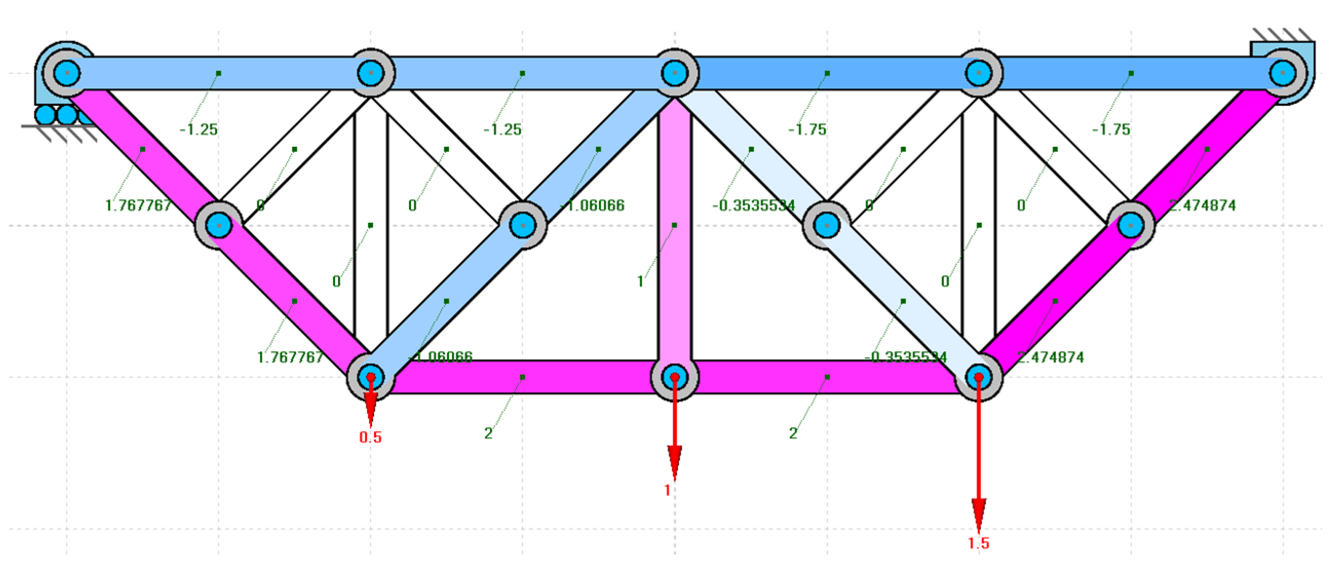
Other standard elements commonly used in dynamic analyses, like springs and dampers, are also implemented in the software to use to model mechanical systems. Because the methodology implemented has a general purpose, it is valid for a system with any number of degrees of freedom, including isostatic structures (mechanical systems with zero degrees of freedom and zero redundancies), such as the one shown in
Figure 15.
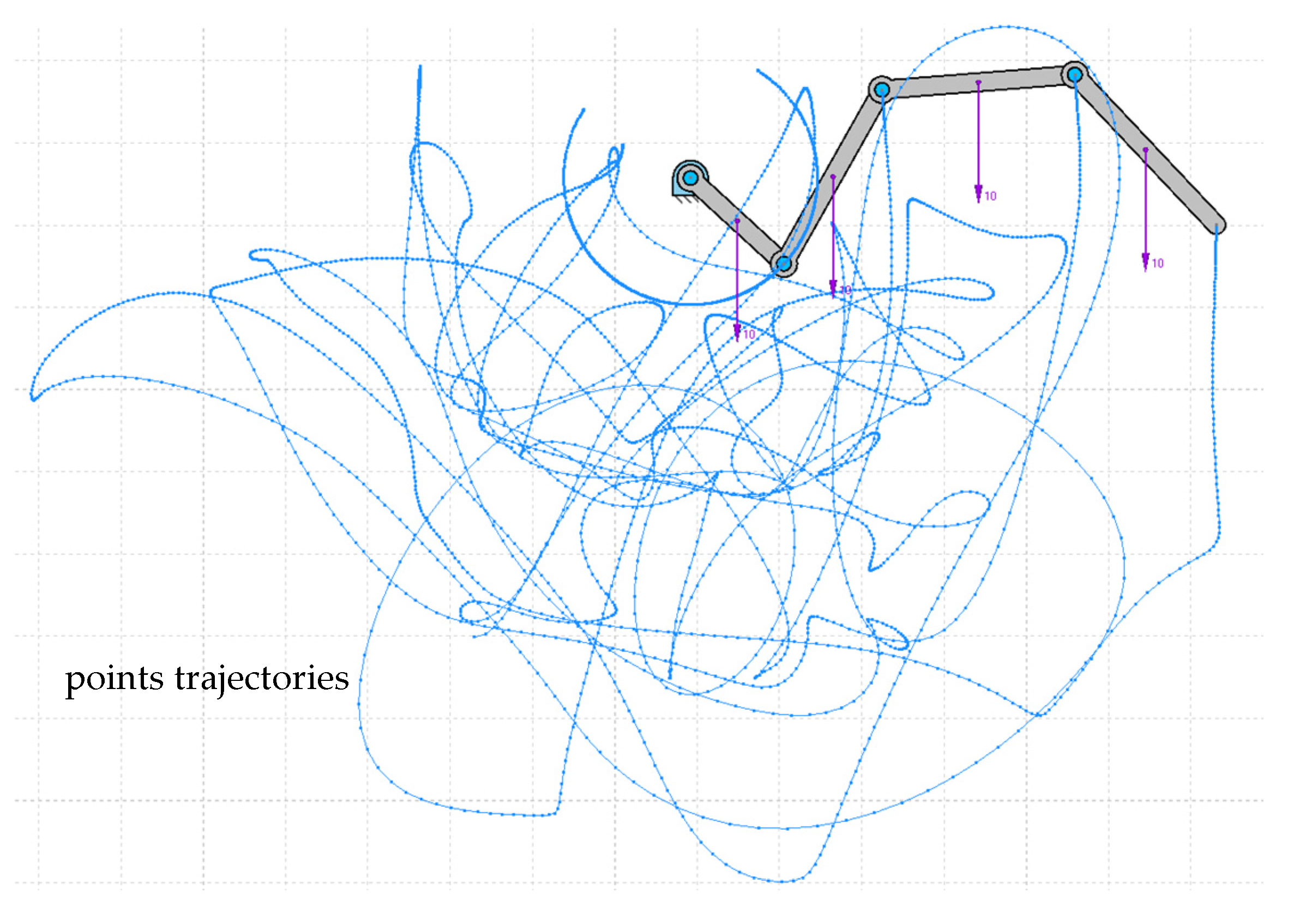
When a direct dynamics problem is computed, the motion is unknown, and simulating it often requires the numerical integration of a system of differential equations because, due to the complexity inherent to the problem, it does not have an analytical solution. This task is programmed in the software, thus students can observe the result (
Figure 16). The motion of the mechanism shown in
Figure 16 can be visualized in the third video included in the
Supplementary Material.
2.4. Synthesis Module
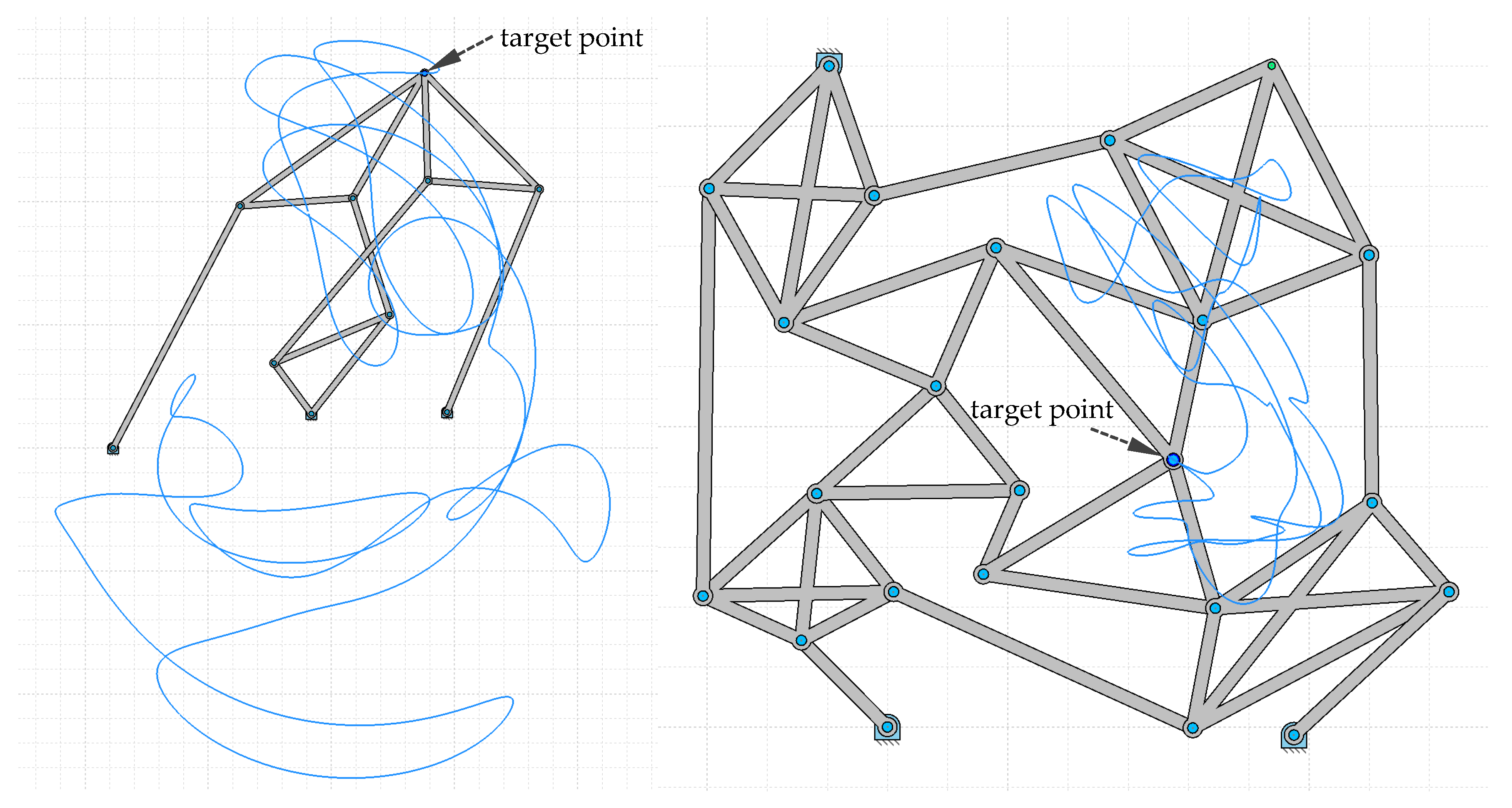
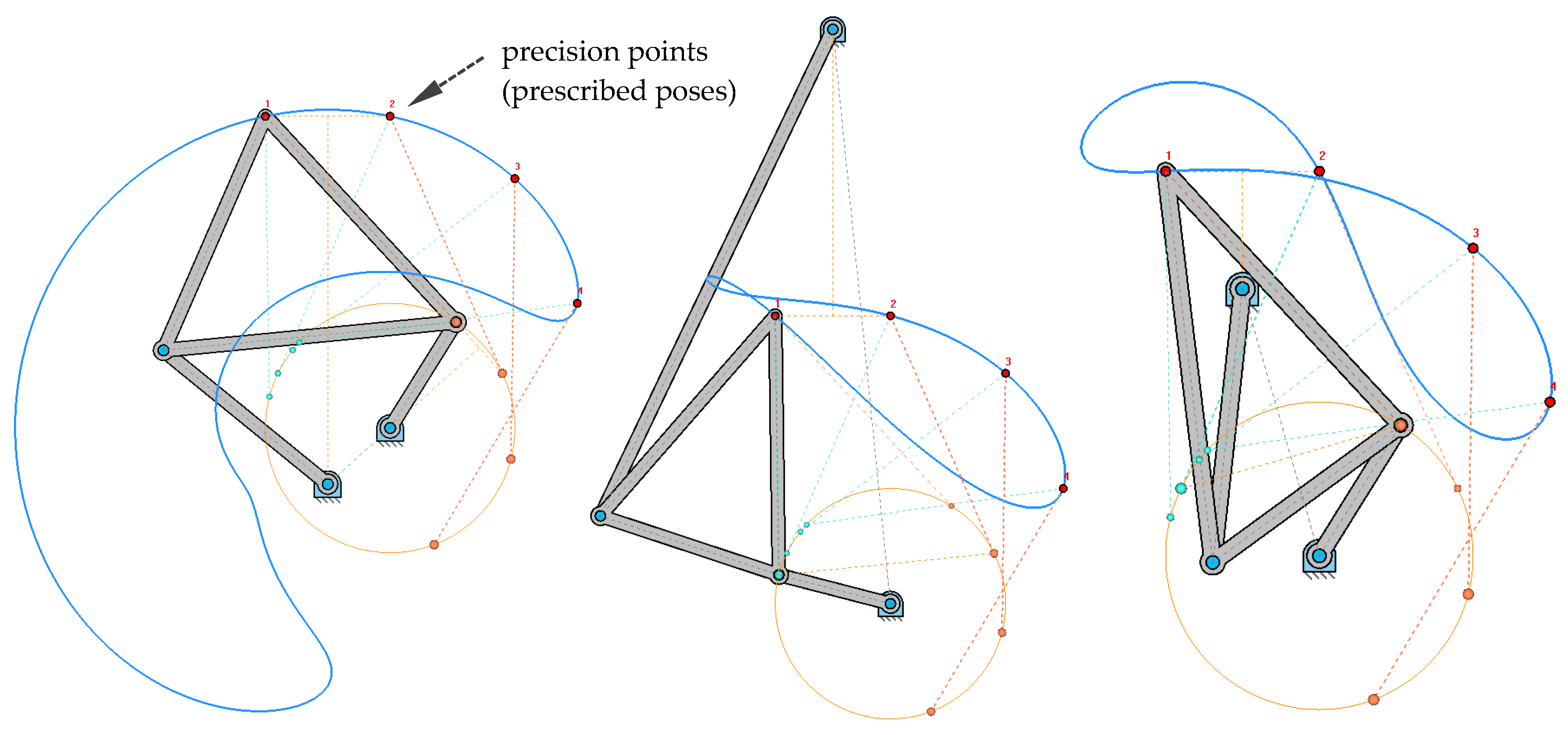
The synthesis module focuses on an approach to teaching based on four-bar linkage. It covers the main types of synthesis, i.e., path generation, rigid body motion, and function generation. Path generation synthesis establishes some precision points that must belong to the trajectory of the four-bar linkage coupler, as shown in
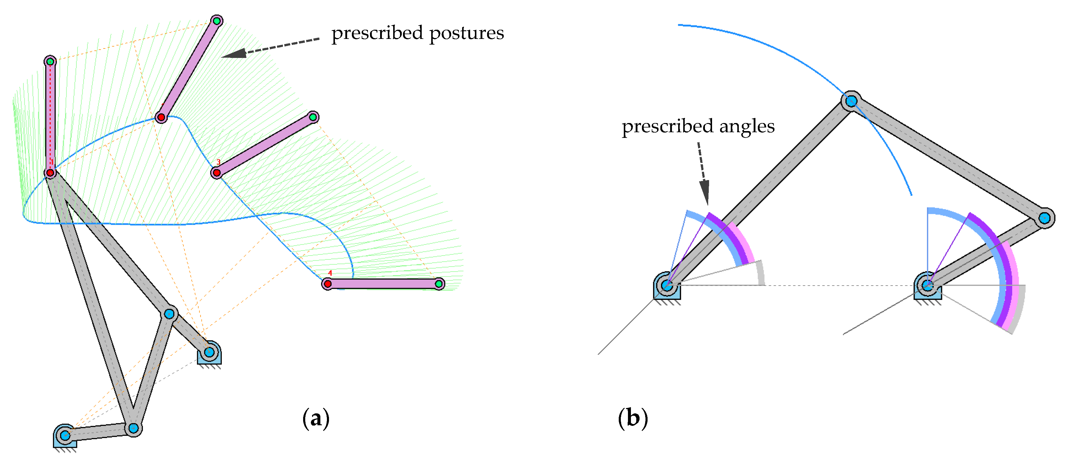
Figure 17. Rigid body motion synthesis establishes poses in which the coupler element must be placed during its motion, as shown in
Figure 18a. Function generation synthesis establishes relations between the angles of input and output that need to be satisfied as shown in
Figure 18b.
For each type of synthesis problem, the interface of the program shows to the student all the graphical constructions required to solve the problem and displays all possible solutions to it, as in the case of a non-linear problem. Students can easily identify such graphical constructions as represented in their handbooks.
In the software, the student can easily change the position of any precision point or any desired posture of the output element, and the impact of this modification in the lengths of the resulting bars is shown in real time.
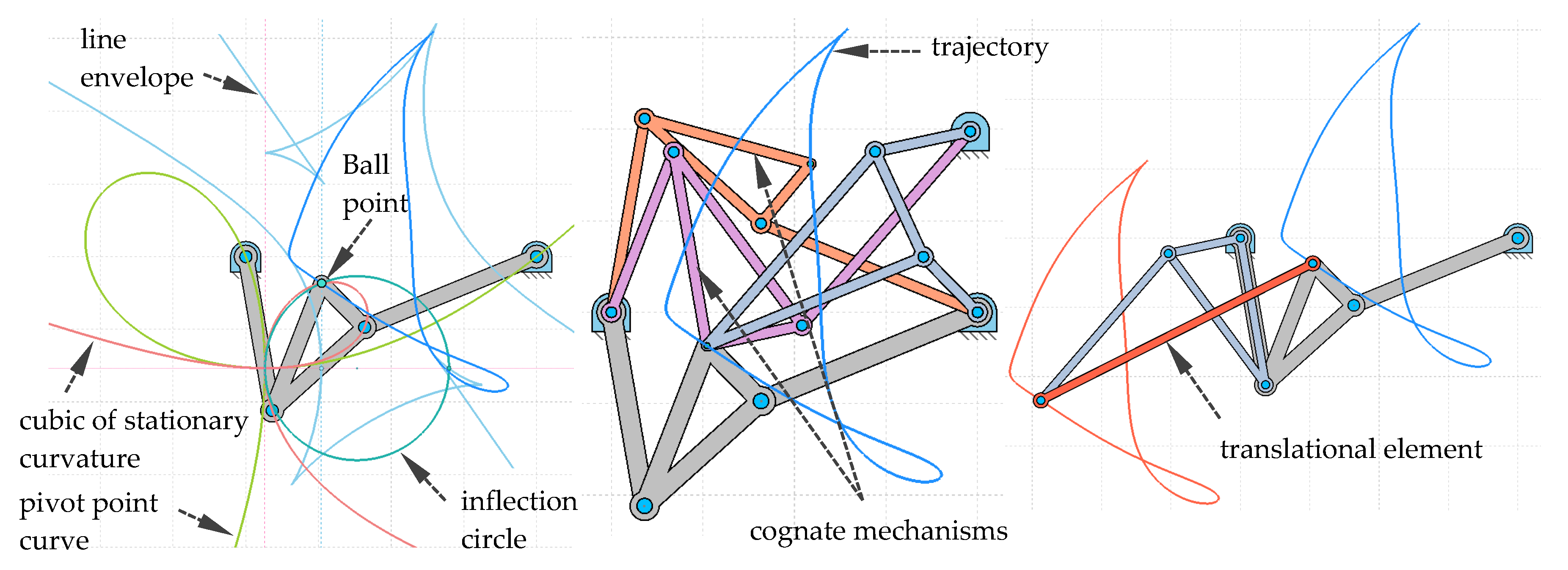
In any synthesis problem, some additional results are provided, such as the line envelope, cubic of stationary curvature, pivot point curve, the Ball point, or cognate mechanisms and their derivations. These are shown in
Figure 19.
3. Active Learning Activities
To highlight the potential of GIM for teaching, different activities performed using it are described in this section. A software can be used to complement and reinforce the complex theoretical concepts of subjects in mechanism and machine science. On the one hand, during academic courses, students have practical sessions in which different exercises are solved using the software. On the other hand, some active learning activities are developed during the seminars for students to enhance their ability to design and analyze different mechanical systems or structures. These activities, commonly known as problem-based learning (PBL), focus on applications. In this way, the students learn to approach problems in engineering.
3.1. Practical Teaching Support Sessions
During an academic course, practical sessions using GIM software are offered to students. In these sessions, lab groups of a maximum of 25 people are created. Initially, the teacher explains in a step-by-step manner the main modules of the GIM software and different options that are implemented. Then, a report template containing some proposed exercises is given to the students. They work independently on their computers, solve the exercises using GIM, and update the report in the Moodle platform for the course once they finish it. Depending on the subject, several problems can be proposed. Some examples are as follows:
Modeling mechanical systems in GIM by first defining the structural diagram of the mechanism being studied and representing it in the Geometry module.
Performing the kinematic analysis of planar or spatial mechanisms to obtain the velocities, accelerations, fixed and moving centrodes, such main circles as inflection, inversion, and cuspidal (or return), and blocking postures. This is done using the Kinematics module.
Making use of the Synthesis module to assess options for the analysis of the four-bar mechanism, such as function generation, path generation, and rigid body motion, to obtain the cognates, and elements with permanent translational motion.
Solving dynamic problems in planar mechanisms to obtain free solid diagrams of elements of the mechanism as well as inner forces and moments.
During these practical sessions, the teacher answers the students’ questions. Once the students have updated their reports to the virtual platform, the teacher reviews them to provide feedback to each student.
3.2. Problem-Based Learning
It is sometimes challenging to capture the interest of students when introducing complex concepts during teaching. Thus, to show them the relation between theory and practice, some case studies based on applications have been developed during seminars. This has helped motivate them to explore different ideas and exercise their creativity [
20].
In general, the methodology followed is as follows: The teacher, at the beginning of the session, explains the case study (the initial data, design criteria, and relevant hints); then, the students work in groups to solve the proposed problem by combining the necessary theoretical developments with the tools offered by GIM. Depending on the difficulty of the case study, this task can be completed during the seminar or finished in the students’ study time. They can then update the report to the Moodle platform within an established period.
A wide variety of practical examples can thus be approached: designing mechanisms to perform certain specific tasks, analyzing the motion of robots and parallel manipulators common in the industry, designing and computing efforts in structures based on trusses, and vibration analysis of simple mechanical systems.
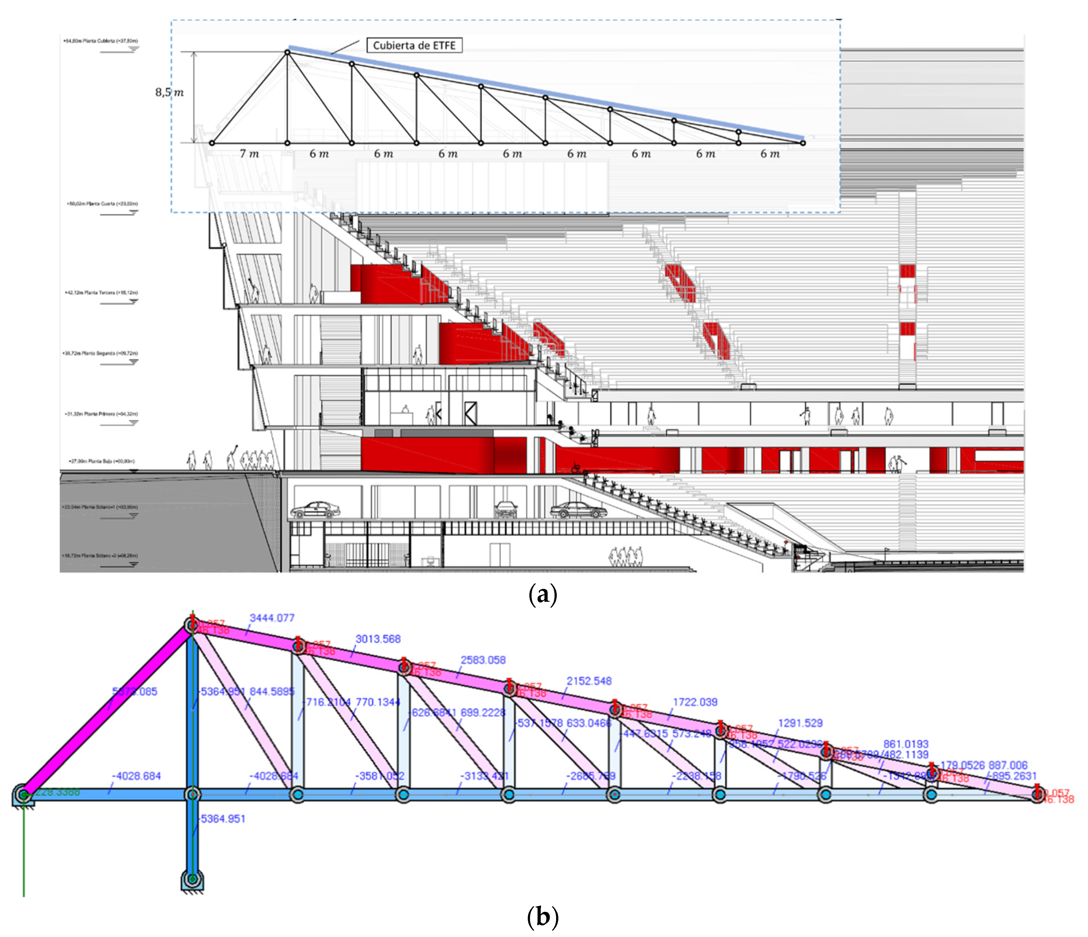
To illustrate the example of a case study proposed during these PBL activities,
Figure 20 shows the rooftop of the San Mamés football stadium in Bilbao (Spain). The stadium is located in front of our university and is very well known to students. The objective of this PBL, which is among the activities designed through an educational innovation project in our Department of Mechanical Engineering (Ref: PIE2012/14), was to tackle the static problem of the truss that conformed to the structure of the rooftop.
Figure 20a shows a floor plan of the truss of the rooftop, and
Figure 20b shows a result obtained by a student. This consisted of reactions under specific loads.
3.3. Self-Learning and Self-Checking
The GIM software is used in practical sessions or seminars that teachers have developed as part of courses that they teach, and any student can install it for free. The website of our research group, COMPMECH Research Group, features a simple user manual to start using the software and many video tutorials to solve different problems with GIM.
Students are encouraged to practice with GIM and make the most of it. Note that the software can act as a self-checking assistant for students. Indeed, students usually take advantage of the software by solving many of the exercises from exams from previous years. They can verify whether their results, obtained by applying the theoretical procedure, coincide with those generated by GIM. In this way, they can identify errors that they made and enhance their skills.
4. GIM in Universities and Companies
The main channel for the dissemination of GIM is the direct download from our COMPMECH research group webpage. In
Table 1, detailed data for downloads of the software to date are presented. The number of institutions adopting GIM has increased over the last few years to more than 500 per year. This software can have a significant positive impact not only on universities and educational centers all over the world, but also on companies and research centers related with innovation and research activities. GIM has also been cited and used in publications related to education and the development of virtual labs [
21,
22,
23,
24,
25].
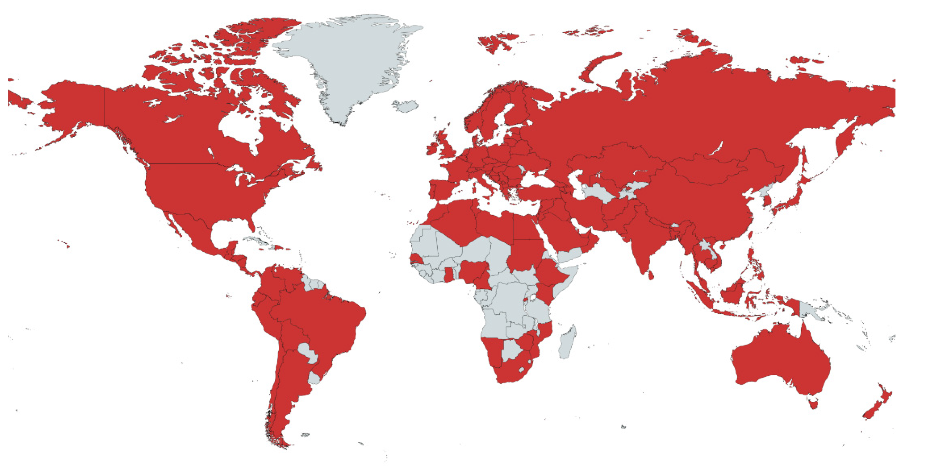
Figure 21 shows the use of the GIM software throughout the world. The countries marked in red are those in which downloads of the software have been registered since 2015.
Tutorials and lectures have been organized to educate the academic community about GIM. In the scope of the IFToMM (International Federation for the Promotion of Mechanism and Machine Science) community, we can cite as instance the tutorial held during the 14th IFToMM World Congress in 2015 in Taipei, and lectures scheduled during IFToMM summer schools (Timisoara 2014 and Palermo 2016). Moreover, in the contexts of the Erasmus + internships and visits to universities, the capabilities of GIM have been presented. This is exemplified by lectures given at the Odessa National Polytechnic University (Ucrania) in 2017, and the presentation given at the Tokyo Institute of Technology in 2019. GIM has been also presented in educational conferences, such as ISEMMS (International Symposium on the Education in Mechanism and Machine Science) [
26] and INTED (International Technology, Education and Development Conference) [
27].
However, a key factor exhibiting the usefulness and interest of the software presented in this paper is the feedback from students that have used it. In an anonymous survey conducted via Google Forms at the end of the academic year 2017–2018 featuring 176 students of the Faculty of Engineering in Bilbao, after having received two lectures (4 h) on the use of the program, 90% stated that the software had been useful for them to better understand the subjects studied (machine theory and applied mechanics). They also highlighted its simplicity of use (91%) and assigned an average score of 3.7/5 to the entire GIM experience.
Recently, in January 2020, an online voluntary and anonymous Google Forms survey was sent to the people that have downloaded the latest version of GIM since September 2019. This survey collected 81 responses. The users’ profile is shown in
Figure 22. As it can be seen, the highest percentage of users is linked to the educational sector as a teacher or a student. This confirms the interest of GIM software as an educational tool. In any case, GIM is also used in companies and for research activities.
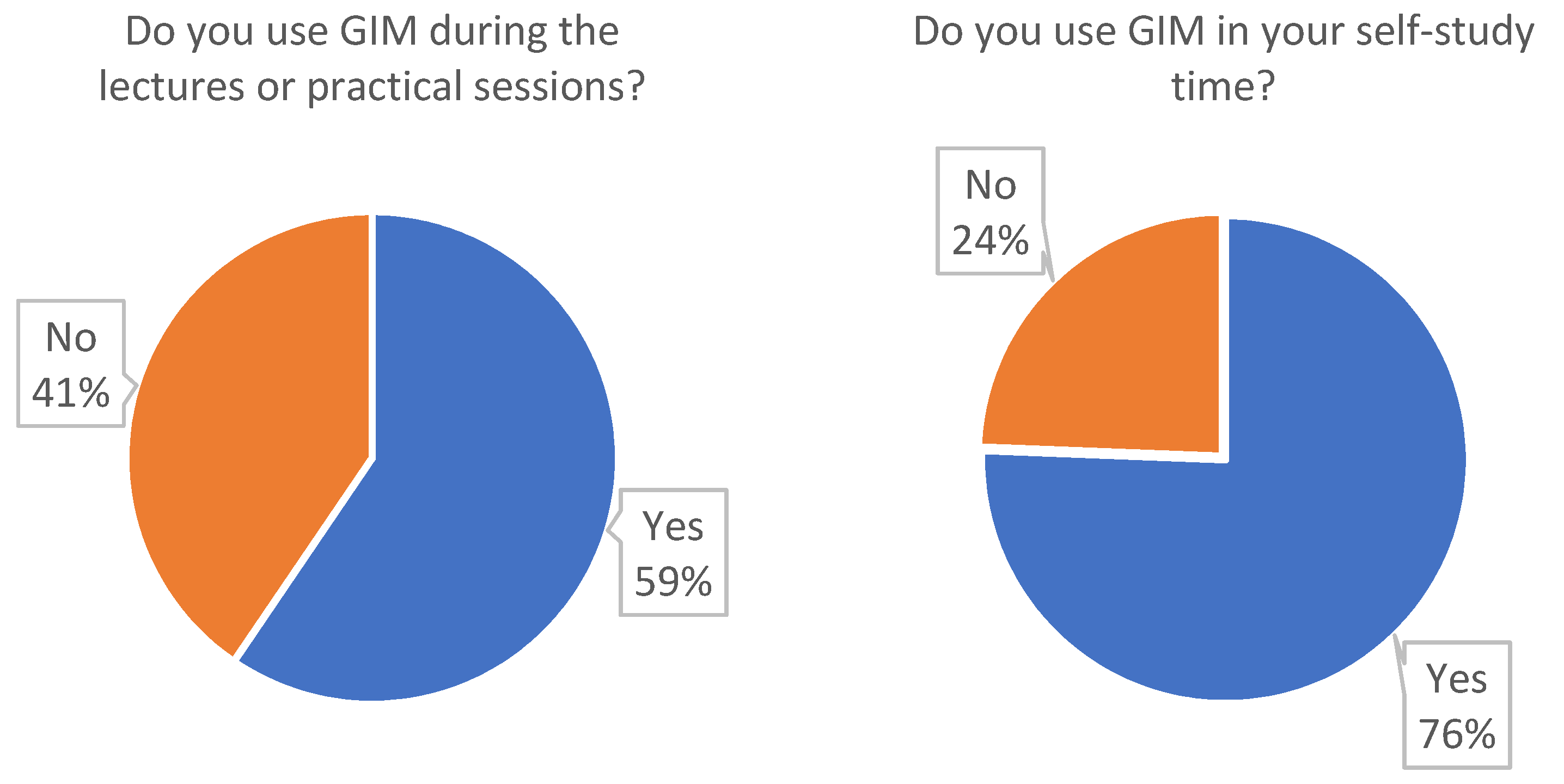
In relation with the use of GIM as a complementary tool for students, the main results are depicted in
Figure 23. It is shown that they use the software not only during the lectures, but also in their self-study time. The students rate the usefulness of GIM as an educational tool with an average rate of 3.9 (scale 0–5).
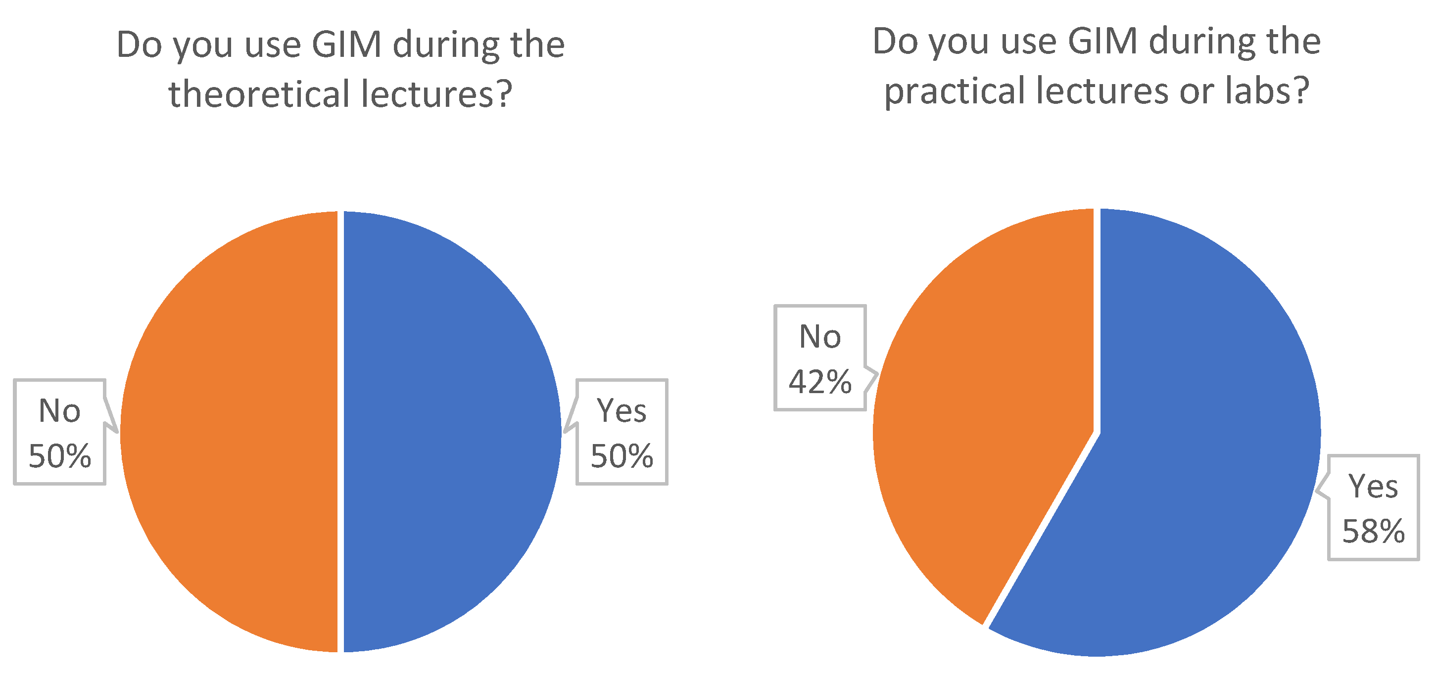
The use of GIM by professors/teachers is shown in
Figure 24. As expected, it has more impact during the practical sessions than in the theoretical lectures. The professors/teachers score the usefulness of GIM as a complement to the lectures with 4.2 (scale 0–5).
The ease of use of GIM is rated by all GIM users with 3.4 (scale 0–5). The score of the overall GIM experience is 3.9 (scale 0–5). Finally, only 6% of the users state that they do not intend to download a future version of GIM. The 68% of the users are sure they will download it and 26% are not sure.
Regarding the specific comments of the users, the negative comments focus on the lack of detailed tutorials for learning how to use all the features offered by the software: “Could really benefit from a comprehensive tutorial”, “Lacking resources to fully utilize all features”, and “Please provide a complete tutorial”. We agree with these comments; the current tutorial is quite brief and the program has much more capabilities than the ones explained in it. We will enhance it by incorporating all the options of GIM.
On the other side, the majority of the comments emphasizes the educational and design capabilities of GIM, such as: “Excellent app to help me understand my course”, “Very interesting software that lets you think directly in the core of the mechanism”, “Plan to have it as an integrated part in my lectures”, and “Wonderful. It is a very effective tool for engineering students and designers”.
5. Conclusions
This paper explored the impact of the GIM software as a supporting tool for teaching university courses on mechanism and machine science. The authors reviewed the potential of the software for modeling planar and spatial linkages, and for carrying out kinematic and dynamic analyses, as well as dimensional synthesis. Although GIM also offers additional, advanced features for PhD Students and other researchers, they are not presented here as they are beyond the scope of the paper.
GIM is being used in many universities as a powerful and valuable tool for boosting students’ learning throughout the academic year. The learning activities presented in the paper show the versatility of GIM and consist of practical and problem-based learning sessions. It is also worth noting the positive effects of the use of the software observed in students in terms of increased motivation for working independently. The feedback received from the students from a survey on the use of GIM reinforced these conclusions.
The impact of GIM was quantified by monitoring direct downloads both from universities (or other educational institutions) and companies or research centers. These downloads have increased annually. In addition, dissemination activities have been organized to present GIM in summer schools, educational conferences, and during lectures in several universities. GIM is constantly evolving to incorporate more capabilities to respond to the demands of different users.
Author Contributions
Conceptualization, V.P.; methodology, E.M.; software, E.M.; validation, M.U.; formal analysis, V.P.; investigation, E.M.; resources, V.P.; data curation, M.U.; writing—original draft preparation, E.M., M.U., V.P., and A.H.; writing—review and editing, M.U.; visualization, M.U.; supervision, A.H.; project administration, A.H.; funding acquisition, A.H. and V.P. All authors have read and agreed to the published version of the manuscript.
Funding
This research was funded by Ministerio de Economía y Competitividad, Spanish Government Project, MINECO/FEDER, UE (grant number DPI2015-67626-P), Departamento de Educación, Política Lingüística y Cultura, Regional Government of the Basque Country (grant number IT949-16) and University of the Basque Country UPV/EHU (grant number PIE2012/14).
Institutional Review Board Statement
Not applicable.
Informed Consent Statement
Not applicable.
Data Availability Statement
Not applicable.
Conflicts of Interest
The authors declare no conflict of interest.
References
- Orlandea, N.; Chace, M.A.; Calahan, D.A. A Sparsity-Oriented Approach to the Dynamic Analysis and Design of Mechanical Systems–Part 1. J. Eng. Ind. 1977, 99, 773. [Google Scholar] [CrossRef]
- Orlandea, N.; Chace, M.A.; Calahan, D.A. A Sparsity-Oriented Approach to the Dynamic Analysis and Design of Mechanical Systems–Part 2. J. Eng. Ind. 1977, 99, 780. [Google Scholar] [CrossRef]
- Levinson, D. AUTOLEV-User’s Manual; Online Dynamics Inc.: Sunnyvale, CA, USA, 1990. [Google Scholar]
- Unda, J.; Avelló, A.; Jiménez, J.M.; García de Jalón, J. COMPAMM-A Program for the Dynamic Analysis of Multi-Rigid-Body Systems. In Engineering Software IV; Springer: Berlin/Heidelberg, Germany, 1985; pp. 983–996. [Google Scholar] [CrossRef]
- Wehage, R.A.; Haug, E.J. Generalized Coordinate Partitioning for Dimension Reduction in Analysis of Constrained Dynamic Systems. J. Mech. Des. 1982, 104, 247. [Google Scholar] [CrossRef]
- Paul, B. DYMAC (Dynamics of MAChinery). In Multibody Systems Handbook; Schiehlen, W., Ed.; Springer: Berlin/Heidelberg, Germany, 1990; pp. 305–322. [Google Scholar]
- Wittenburg, J.; Wolz, U. MESA-VERDE a Symbolic Program for Nonlinear Articulated Rigid-Body Dynamics. In Proceedings of the ASME Design Engineering Technical Conference, Cincinnati, OH, USA, 10–13 September 1985; Volume 8. [Google Scholar]
- Suñer, J.L.; Carballeira, J. Enhancing Mechanism and Machin Science Learning by Creating Virtual Labs with ADAMS. In New Trends in Educational Activity in the Field of Mechanism and Machine Theory; García-Prada, J.C., Castejón, C., Eds.; Springer: Berlin/Heidelberg, Germany, 2014; pp. 221–228. [Google Scholar]
- Rubel, A.J.; Kaufman, R.E. KINSYN III: A new human-engineered system for interactive computer-aided design of planar linkages. J. Eng. Ind. Trans. ASME 1977, 99, 440–448. [Google Scholar] [CrossRef]
- Erdman, A.G.; Gustafson, J. LINCAGES: A linkage interactive computer analysis and graphically enhanced synthesis package. In Proceedings of the ASME Design Engineering Technical Conferences, 77-DTC-5, Chicago, IL, USA, 26–30 September 1977. [Google Scholar]
- Chuang, J.C.; Strong, R.T.; Waldron, K.J. Implementation of solution rectification techniques in an interactive linkage synthesis program. J. Mech. Des. 1981, 103, 657–661. [Google Scholar] [CrossRef]
- Müller, M.; Mannheim, T.-P.; Hüsing, M.; Corves, B. MechDev-A new Software for Developing Planar Mechanisms. In Interdisciplinary Applications of Kinematics. Mechanisms and Machine Science; Kecskeméthy, A., Geu Flores, F., Carrera, E., Elias, D., Eds.; Springer: Berlin/Heidelberg, Germany, 2018; Volume 71, pp. 167–175. [Google Scholar]
- Bataller, A.; Ortiz, A.; Cabrera, J.A.; Nadal, F. WinMecC: Software for the Analysis and Synthesis of Planar Mechanisms. In New Trends in Mechanism and Machine Science, Mechanism and Machine Science; Wenger, P., Flores, P., Eds.; Springer: Berlin/Heidelberg, Germany, 2017; Volume 43, pp. 233–242. [Google Scholar]
- Nadal, F.; Cabrera, J.A.; Bataller, A.; Castillo, J.J.; Ortiz, A. Turning functions in optimal synthesis of mechanisms. J. Mech. Des. 2015, 137, 6. [Google Scholar] [CrossRef]
- Technologies, Design Simulation. Working Model. 2007–2012. Available online: https://www.design-simulation.com/ (accessed on 26 August 2021).
- Hohenwarter, M.; Preiner, J. Dynamic mathematics with GeoGebra. J. Online Math. Its Appl. 2007, 7, 1448. [Google Scholar]
- Calvo, J.A.; Álvarez-Caldas, C.; San Román, J.L. Analysis of Dynamic Systems Using Bond Graph and SIMULINK. In New Trends in Educational Activity in the Field of Mechanism and Machine Theory; García-Prada, J.C., Castejón, C., Eds.; Springer: Berlin/Heidelberg, Germany, 2014; pp. 155–162. [Google Scholar]
- García de Jalón, J.; Callejo, A. A straight methodology to include multibody dynamics in graduate and undergraduate subjects. Mech. Mach. Theory 2011, 46, 168–182. [Google Scholar] [CrossRef]
- Petuya, V.; Macho, E.; Altuzarra, O.; Pinto, C.; Hernández, A. Educational software tools for the kinematic analysis of mechanisms. Comput. Appl. Eng. Educ. 2014, 22, 72–86. [Google Scholar] [CrossRef]
- Royalty, A. Design-base d Pedagogy: Investigating an emerging approach to teaching design to non-designers. Mech. Mach. Theory 2018, 125, 137–145. [Google Scholar] [CrossRef]
- Hamon, C.L.; Green, M.G.; Dunlap, B.; Camburn, B.A.; Crawford, R.H.; Jensen, D.D. Virtual or physical prototypes? Development and testing of a Prototyping Planning Tool. In Proceedings of the 121st ASEE Annual Conference and Exposition, Indianapolis, IN, USA, 15–18 June 2014. [Google Scholar]
- Wang, Y.; Ong, S.K.; Nee, A.Y.C. Enhancing mechanisms education through interaction with augmented reality simulation. Comput. Appl. Eng. Educ. 2018, 26, 1552–1564. [Google Scholar] [CrossRef]
- Adrian, P.; Reinoso, O.; Gil, A. A virtual laboratory to simulate the control of parallel robots. In Proceedings of the 3rd IFAC Workshop on Internet Based Control Education (IBCE 2015), Brescia, Italy, 4–6 November 2015; Volume 48, pp. 19–24. [Google Scholar]
- Hampali, S.; Chittawadigi, R.G.; Saha, S.K. MechAnalyzer. 3D Model Based Mechanism Learning Software. In Proceedings of the 14th IFToMM World Congress, Taipei, Taiwan, 25–30 October 2016; pp. 425–431. [Google Scholar]
- Craifaleanu, A.; Dragomirescu, C.; Craifaleanu, I.G. Virtual Laboratory of Dynamics. In Proceedings of the 6th International Conference on Education and New Learning Technologies (EDULEARN), Barcelona, Spain, 7–9 July 2014; pp. 4612–4619. [Google Scholar]
- Urízar, M.; Altuzarra, O.; Diez, M.; Campa, F.J.; Macho, E. Dynamics and Mechanical Vibrations. Complementing the Theory with Virtual Simulation and Experimental Analysis. In New Trends in Educational Activity in the Field of Mechanism and Machine Theory; García-Prada, J.C., Castejón, C., Eds.; Springer: Berlin/Heidelberg, Germany, 2019; pp. 64–71. [Google Scholar]
- Petuya, V.; Altuzarra, O.; Pinto, C.; Hernández, A. A new educational software for the kinematic analysis of spatial mechanisms. In Proceedings of the International Technology, Education and Development Conference (INTED 09), Valencia, Spain, 9–11 March 2009; ISBN 978-84-612-7578-6. [Google Scholar]
Figure 1.
Proposed case study.
Figure 1.
Proposed case study.
Figure 2.
Main steps of geometric definition: 1—Nodes, 2—Elements, 3—Joints.
Figure 2.
Main steps of geometric definition: 1—Nodes, 2—Elements, 3—Joints.
Figure 3.
Planar joints implemented in GIM.
Figure 3.
Planar joints implemented in GIM.
Figure 4.
Spatial joints implemented in GIM.
Figure 4.
Spatial joints implemented in GIM.
Figure 5.
Position of a point in spherical coordinates.
Figure 5.
Position of a point in spherical coordinates.
Figure 6.
Main kinematic results: Trajectories, velocities, and accelerations for given inputs.
Figure 6.
Main kinematic results: Trajectories, velocities, and accelerations for given inputs.
Figure 7.
Visualizing decomposition of velocity and acceleration.
Figure 7.
Visualizing decomposition of velocity and acceleration.
Figure 8.
Disk element fixed and moving centrodes in absolute and relative motions. Velocities of poles.
Figure 8.
Disk element fixed and moving centrodes in absolute and relative motions. Velocities of poles.
Figure 9.
Angular velocities and accelerations. Loci of center of curvature of a trajectory.
Figure 9.
Angular velocities and accelerations. Loci of center of curvature of a trajectory.
Figure 10.
Swept of revolute joint axis swept. Element’s swept. Fixed and moving axodes with the instantaneous axes of rotation and sliding.
Figure 10.
Swept of revolute joint axis swept. Element’s swept. Fixed and moving axodes with the instantaneous axes of rotation and sliding.
Figure 12.
Value of driving load for the computation of inverse dynamics.
Figure 12.
Value of driving load for the computation of inverse dynamics.
Figure 13.
Free solid and internal efforts’ diagrams.
Figure 13.
Free solid and internal efforts’ diagrams.
Figure 14.
Color map of internal effort for all systems and evolution over time for an element.
Figure 14.
Color map of internal effort for all systems and evolution over time for an element.
Figure 15.
Axial forces of isostatic structure.
Figure 15.
Axial forces of isostatic structure.
Figure 16.
Simulating the motion of a chain released to the effect of gravity from repose.
Figure 16.
Simulating the motion of a chain released to the effect of gravity from repose.
Figure 17.
Path planning synthesis; multiple solutions.
Figure 17.
Path planning synthesis; multiple solutions.
Figure 18.
Rigid body motion (a) and function generation (b) synthesis.
Figure 18.
Rigid body motion (a) and function generation (b) synthesis.
Figure 19.
Line envelope, cubic of stationary curvature, pivot point curve, and Ball point. Cognates and derived translational mechanism.
Figure 19.
Line envelope, cubic of stationary curvature, pivot point curve, and Ball point. Cognates and derived translational mechanism.
Figure 20.
Example of PBL: (a) Rooftop of the football stadium in Bilbao (Spain), (b) Results.
Figure 20.
Example of PBL: (a) Rooftop of the football stadium in Bilbao (Spain), (b) Results.
Figure 21.
Countries using GIM software.
Figure 21.
Countries using GIM software.
Figure 22.
GIM users’ profile.
Figure 22.
GIM users’ profile.
Figure 23.
Use of GIM in the learning process.
Figure 23.
Use of GIM in the learning process.
Figure 24.
Use of GIM in the teaching process.
Figure 24.
Use of GIM in the teaching process.
Table 1.
GIM download data.
Table 1.
GIM download data.
| Academic Year | Institutions | Countries | Universities or Other Educational Institutions | Companies or Research Centers |
|---|
| 2015/2016 | 341 | 66 | 248 | 93 |
| 2016/2017 | 551 | 90 | 417 | 134 |
| 2017/2018 | 560 | 88 | 395 | 165 |
| 2018/2019 | 502 | 86 | 376 | 126 |
| 2019/2020 | 660 | 92 | 516 | 144 |
| Publisher’s Note: MDPI stays neutral with regard to jurisdictional claims in published maps and institutional affiliations. |
© 2021 by the authors. Licensee MDPI, Basel, Switzerland. This article is an open access article distributed under the terms and conditions of the Creative Commons Attribution (CC BY) license (https://creativecommons.org/licenses/by/4.0/).


