Lifetimes of Used Nuclear Fuel Containers Affected by Sulphate-Reducing Bacteria Reactions inside the Canadian Deep Geological Repository

Abstract

The present work aims at approximating the reduction of sulphate to sulphide caused by sulphate-reducing bacteria (SRB) inside the Canadian deep geological repository in order to calculate the expected lifetime of used nuclear fuel containers (UFCs). Previous studies have assumed a conservative constant concentration of sulphide at the host rock interface. The novelty of this study resides in the use of first-order kinetics to explicitly account for the SRB-induced sulphide production. This reaction term is developed following an empirical approach using published results on actual sulphate reduction by SRB and included in a coupled reaction-diffusion system. Lifetimes of UFCs are subsequently calculated following the conditions of two scenarios: having SRB active only at the region closest to the host rock and having SRB active at the host rock and throughout the bentonite clay. This study shows that the mean lifetimes of UFCs in both cases are above one million years. However, more accurate results would require the characterization of the host rock and groundwater of the prospective emplacement, as well as additional experiments on growth and sulphide production by the microbial communities from the site.

1. Introduction

Deep geological repositories (DGR) are considered the safest long-term nuclear waste disposal solution [1]. They involve the excavation of an underground site where used fuel containers (UFC) are placed for permanent storage. The basic idea of the design is to use several barriers of different materials to protect and contain the UFCs. A number of countries are currently developing DGRs, among them are Finland, Sweden, and Canada [2,3,4].

The Canadian DGR design is planned to host approximately 4.6 million CANDU (Canada Deuterium Uranium) used fuel bundles contained within 96,000 UFCs in a suitable rock formation, either crystalline or sedimentary. The vaults containing the UFCs will be located at a depth of about 500 m underground [5]. The design is based on a multiple-barrier system which is designed to contain and isolate the nuclear waste. Two important layers of protection in this system are provided by the UFCs and the highly compacted bentonite (HCB). The UFCs are 2.5 × 0.556 × 0.556 [m] canisters made of steel with a 47-mm-thick cylindrical shell with 30-mm-thick hemispherical caps and an external 3-mm-thick copper coating [5]. The HCB is an absorbent aluminum phyllosilicate clay that has been compacted to achieve a designed dry density and is the material responsible for isolating the UFCs from the host rock of the vault and preventing any inflow or outflow of materials. Bentonite swells upon contact with water which makes it a natural water barrier and a sealer to the placement rooms. Buffer boxes made of HCB are created to enclose the UFCs, these boxes are then placed inside the placement rooms. The space between the buffer boxes and the host rock is backfilled with bentonite pellets dubbed ‘gapfill’ in this work (Figure 1).

Modelling Scope and Container Failure

Mass transport inside the DGR is an important process closely connected to the safety of its design, whether the inward transport of corrosive species [6,7] or the outward transport of radionuclides [8,9], the capacity of the engineered barriers to block the mobility of chemical species is tightly connected to the long term safety of the DGR. In the Canadian DGR design, the inward transport of sulphide has assumed a constant concentration of sulphide at the rock interface [6]. A value of 3 ppm (9.07 × 10⁻⁵ M) has been deemed conservative as the stringent conditions of high pressure and low available water would limit bacterial growth [6]. However, so far, this constraining process has not been explicitly included in the mass transport models. Having a source term would provide information about the transient stage inside the placement room and be a step towards a more realistic and comprehensive model.

Three-dimensional models of the placement rooms show that the flux of sulphide from the host rock to the UFCs is higher at the hemispherical ends [6]. Therefore, in the present work, a one-dimensional model of the section that goes from the host rock to the endcap of the UFC is developed.

Container failure is defined as the through-wall penetration of the outer protective layer [10], i.e., the 3-mm-thick copper layer. Other definitions of failure exist, such as plastic deformation, brittle, or ductile fracture; however, since the focus of this study is the mass transport of corrosive species, the former definition is adopted.

2. Reaction-Diffusion Model

2.1. Reaction-Diffusion System

The system proposed to describe the production of sulphide by the SRB and its dispersion over a one-dimensional space is a set of coupled reaction–diffusion equations:

$$\{\begin{array}{c}\frac{\partial S}{\partial t}=D_S\left(k_{\rho }\right) \frac{{\partial }^{2}S}{\partial x^2}-R\left(k_{\rho },S\right)\\ \frac{\partial H}{\partial t}=D_H\left(k_{\rho }\right) \frac{{\partial }^{2}H}{\partial x^2}+R\left(k_{\rho },S\right).\end{array}$$

(1)

Initial and boundary conditions are given and presented in the next section; S stands for the concentration of sulphate, $\left[S{O}_4^{2-}\right]$, and H for that of sulphide $\left[H{S}^{-}\right]$; the reaction or source term $R\left(k_{\rho },S\right)$ is a function of the bentonite dry density and the concentration of sulphate; and the diffusion coefficients are also a function of the dry density of the bentonite.

The reaction term is assumed to be a first-order chemical reaction that approximates the reduction of sulphate to sulphide by the SRB and whose reaction rate constant is obtained from an optimization procedure applied to published experimental results as shown in Section 3.

The reaction–diffusion system of Equation (1) is implemented and solved using a one-dimensional finite-difference model in MATLAB^®. Since the model is intended to produce several thousand runs, an experiment is developed to find a balance between accuracy and computation time. The accuracy of the solution is mainly determined by the spatial increment ∆x; therefore, the experiment solves the reaction-diffusion model for different spatial increments and the criterion for selecting the optimal size of ∆x is the minimal computation time such that its accuracy does not deviate more than 0.5% with respect to the most accurate lifetime solution (see Appendix A).

2.2. Initial and Boundary Conditions

A sharp hydraulic gradient would exist between the pressure of the geosphere and the atmospheric pressure of the placement rooms of the DGR [11]. Groundwater would seep into a repository and saturate the gapfill and the HCB. Therefore, the initial and boundary conditions of the model are given by the composition and concentration of the chemical species in the groundwater of the host rock. Currently, no final location for the DGR has been selected and, therefore, no sample analysis has been performed. There exists, however, reference groundwater concentrations for crystalline and sedimentary rock at approximately 500 m underground [12]. The concentrations of sulphate and sulphide are taken as input values to calculate the boundary conditions and are shown in

Table 1. Groundwater composition [mg/L].

Rock Type	Sulphate	Sulphide
Crystalline	1000	0
Sedimentary	310	0

.

Initial conditions for both chemicals are assumed to be zero, other saturation conditions were tested but they do not significantly affect the sulphide flux to the UFC or their lifetimes. The left-hand side (LHS) boundary condition for sulphate is kept constant at the given reference concentration of Table 1 and its right-hand side (RHS) boundary is given by the Neumann boundary condition:

$$\frac{\partial S\left(L,t\right)}{\partial x}=0, \forall t,$$

i.e., the RHS acts as a physical barrier.

For sulphide, it is assumed that the host rock would act as a physical barrier preventing any sulphide from leaving the system and, therefore, the LHS boundary is defined using the Neumann boundary condition

$$\frac{\partial H\left(0,t\right)}{\partial x}=0, \forall t.$$

The RHS boundary for sulphide is kept constant at a concentration of zero, following the conservative assumptions in [6,13] that copper corrosion is mass-transport limited and that any sulphide molecules reaching the surface of the UFC will instantly corrode the copper layer.

2.3. Effective Diffusivity

The effective diffusivity of sulphide anions is taken from [14], which made the effective diffusivity depend on the bentonite dry density as follows

$$D_e=5.30087\times {10}^{-10} exp\left(-2.561\times {10}^{-3}{\rho }_{Dry}\right)$$

(2)

were the effective diffusivity ($D_e$) is in units [m²/s] and the dry density of the bentonite (${\rho }_{Dry}$) has units [kg/m³]. For the effective diffusivity of sulphate, this work follows [15] using half the value of the sulphide diffusivity.

Table 2. Bentonite clay properties.

	Dry Density [kg/m3]	Porosity %	Saturation %	Sulphide DH [m2/s]	Sulphate DS [m2/s]
Gapfill	1410	48.6	6	1.43 × 10−11	7.15 × 10−12
HCB	1700	38.2	67	6.81 × 10−12	3.40 × 10−12

shows the properties and diffusivities for the designed densities of the bentonite clay in the Canadian DGR.

3. Sulphate-Reducing Bacteria Activity

The chemical reaction describing the sulphate-reducing mechanism [16] carried out by sulphate-reducing bacteria (SRB) is the following

$$4{\mathrm{H}}_2+{\mathrm{SO}}_4^{2-}+{\mathrm{H}}^{+}\to {\mathrm{HS}}^{-}+4{\mathrm{H}}_2\mathrm{O}$$

(3)

This chemical reaction is likely non-elementary; however, under the assumption of an abundance of hydrogen gas (H₂) and hydrogen ions (H⁺), it can be approximated by an elementary first-order reaction. In [17] is shown that the reduction of sulphide into sulphide can indeed be approximated by first-order kinetics.

The procedure adopted in this work is to use a two-step process to model SRB activity. First, a first-order kinetics is found from experimental results about sulphate reduction under favorable laboratory conditions using SRB microorganisms extracted from a deep bedrock [18,19]. Then, the kinetic constant is adjusted to match experimental results made under conditions similar to those present inside the DGR [20].

3.1. SRB-Driven Sulphate Reduction

Data was used from [18,19], who performed an experiment to study copper corrosion on the presence and absence of SRB. Copper specimens were exposed to biotic and abiotic artificial anoxic groundwaters for periods of 4 and 10 months and then examined their chemical and electrochemical changes. The microorganisms used in the experiment came from the deep bedrock of Olkiluoto, Finland.

A particular featured of the results is that pH decreased after the experiment, meaning that the concentration of hydrogen ions increased, since $\left[{\mathrm{H}}^{+}\right]={10}^{-\mathrm{pH}}$ (from pH = −log₁₀[H⁺]). A decrease in hydrogen ions was expected in reaction (3) under controlled conditions, indicating that likely other reactions took place which increased the hydrogen ion concentration.

Therefore, since hydrogen ions were not limiting the reaction, it was assumed that hydrogen ions would be in abundance for groundwater with similar characteristics. This is a conservative, bounding scenario as the real rate of sulphide production will be significantly less than this. Additionally, the electrolysis of water into hydrogen gas (H₂) and oxygen (O₂) was assumed to be faster than the sulphate reduction to represent a conservative scenario; therefore, hydrogen gas was also considered in abundance inside the DGR. However, the use of HCB would prevent the formation of a biofilm on the surface of the UFCs as it did in the experiments; therefore, this sulphide production rate is an extreme bounding case representing the worst-case scenario in which every engineered barrier system fails [20]

The conservative bounding upper limit of the reaction rate is described by

$$\frac{\partial S}{\partial t}=-k_{\rho }S$$

(4a)

$$\frac{\partial H}{\partial t}=\chi k_{\rho }H$$

(4b)

where $k_{\rho }$ is the reaction rate coefficient as a function of the dry density ${\rho }_{dry}$, χ is the efficiency of the reaction, and S and H are concentrations in [mol/L]. If concentrations were in [mg/L], then the right-hand side of Equation (4b) must be multiplied by the factor 33.07/96.06 to account for the mole conversion.

3.2. Reaction Rate Constant

The analytical solution of (4a) describes an exponential decay:

$$S=a_{0}exp\left(-k_{\rho }t\right)$$

(5)

where $a_0$ can be determined from the initial conditions and for $k_{\rho }$ an optimization procedure was used to find the optimal value of $k_{\rho }{}^{*}$ that minimizes the error of the predicted reduction with respect to the observed data. Two objective functions are tested, the squared differences and the square of log differences.

$$\begin{array}{c}\{\begin{array}{l}\underset{k_{\rho }}{\mathrm{Min}}{\displaystyle {\displaystyle \sum }_i}{\left(d_i-{\widehat{d}}_i\right)}^2\hfill \\ s.t.\hfill \\ {\widehat{d}}_i=a_0\exp \left(-k_{\rho }{t}_i\right), \forall i \hfill \end{array}\end{array}$$

(6)

The optimization model (6) is minimized using the bracketing method, which is an iterative approach and where $d_i$ is the concentration of $S{O}_4^{2-}$ after time $t_i$ obtained from the experiment. This model yields an optimal kinetic constant of $k_{\rho }{}^{*}=5.9631\times {10}^{-9}\left[1/s\right]$.

The second optimization model:

$$\begin{array}{c}\{\begin{array}{l}\underset{k_{\rho }}{\mathrm{Min}}\frac{1}{2}{\displaystyle {\displaystyle \sum }_i}{\left[ln\left(d_i\right)-ln\left({\widehat{d}}_i\right)\right]}^2\hfill \\ s.t.\hfill \\ ln\left({\widehat{d}}_i/a_0\right)=-k_{\rho }{t}_i, \forall i \hfill \\ k_{\rho }\ge 0\hfill \end{array}\end{array}$$

(7)

has a closed optimal solution given by

$$k_{\rho }=\frac{{{\displaystyle \sum }}_i{t}_i ln\left(\raisebox{1ex}{$a_0$}\!\left/ \!\raisebox{-1ex}{$d_i$}\right.\right)}{{{\displaystyle \sum }}_i{t}_i{}^2}$$

and the optimal kinetic constant in this model is $k_{\rho }{}^{*}=6.1614\times {10}^{-9}\left[1/s\right]$. This rate constant is adopted since it refers to the most unsafe situation and because it yielded a smaller error in two out of three error measures (see Appendix A).

Therefore, the optimal reduction of sulphate describing the results from experiments in [18,19] is

$$\frac{\partial S}{\partial t}=-6.16\times {10}^{-9} S$$

(8)

in units [M/s].

3.3. Efficiency of the Reaction

Using the same experimental results from [18,19] and reaction (3), the theoretical sulphide production from the stoichiometry is calculated and compared with the actual sulphide production to determine the efficiency of the reaction. The theoretical production is 34.6 [mg/L] and the actual production is approximately 14.14 [mg/L]; therefore, the efficiency of the kinetics is

$$\chi =\frac{14.14\left[\frac{\mathrm{mg}}{\mathrm{L}}\right]}{34.6\left[\frac{\mathrm{mg}}{\mathrm{L}}\right]}=\mathrm{0.408.}$$

(9)

3.4. Suppressing Effect of Bentonite Dry Density

Since the extreme pressure conditions inside the DGR differ from those on the experiments [18,19], the reaction rate constant of Equation (8) is adjusted using the dry density of the bentonite as a suppressive factor because it determines the pore size of the clay and the swelling pressure which are two major factors limiting SRB activity.

An exponential functional form is selected to attenuate the reaction rate constant as experiments have shown that the swelling pressure of bentonite increases exponentially with respect to the dry density of the bentonite clay [11]. The exponential form developed must meet the following conditions

• $k_A\left({\rho }_R\right)=k_{\rho }$, i.e., the reaction constant under the baseline density of the experiment of Section 3.2 must equal the optimal reaction constant of Equation (8).

• $k_A\left({\rho }_S\right)=0$, i.e., if the dry density equals the specific density of the bentonite clay $\left({\rho }_S=2760 \left[\mathrm{kg}/{\mathrm{m}}^3\right]\right)$, then the reaction constant becomes zero as there is no pore space available for bacteria to remain active.

The exponential form developed is

$$k_A\left({\rho }_{Dry}\right)=\left[{\left(\frac{k_{\rho }}{C_f}+1\right)}^{\frac{{\rho }_S-{\rho }_{Dry}}{{\rho }_S-{\rho }_0}}-1\right]C_f, {\rho }_{Dry}\in \left[{\rho }_0, {\rho }_S\right]$$

(10)

where $k_A\left({\rho }_{Dry}\right)$ is the attenuated or adjusted rate, ${\rho }_{Dry}$ is the dry density of the clay in [kg/m³] and $C_f$ is a value at which the rate constant is taken to be zero (details on the derivation of this formula are presented in [21]). Sulphate to sulphide reduction rates estimated by [22] are used to determine the value of $C_f$ that best approximate the sulphide production on those experiments.

Therefore, an optimization model is created to find the optimal value of $C_f$ matches the sulphide reduction presented in [22]. The model is the following

$$\begin{array}{c}\{\begin{array}{l}\underset{C_f}{\mathrm{Min}}{\displaystyle {\displaystyle \sum }_i}{\left(k_D{}^{\left(i\right)}-k_A{}^{\left(i\right)}\right)}^2\hfill \\ s.t.\hfill \\ k_A{}^{\left(i\right)}=\left[{\left(\frac{k_{\rho }}{C_f}+1\right)}^{\frac{{\rho }_S-{\rho }_{Dry}{}^{\left(i\right)}}{{\rho }_S-{\rho }_0}}-1\right]C_f.\hfill \end{array}\end{array}$$

(11)

Gradient descent, which is an iterative approach to solve optimization problems, is used to find the optimal value for $C_f$ yielding an optimal value of $C_f{}^{*}=1.37\times {10}^{-17} \left[1/s\right]$. The attenuated reaction rate constants are shown in

Table 3. Attenuated reaction rate constant.

Clay	Dry Density [kg/m3]	Rate Attenuated kA [1/s]
Gapfill	1410	7.33 × 10−11
HCB	1700	3.19 × 10−12

.

3.5. Lifetimes Calculations

Sulphide flux to the UFC is calculated following Fick’s first law of diffusion at the RHS boundary and time t of the simulation using:

$$J\left(L,t\right)=-D_H\frac{\partial H}{\partial x}, \forall t,$$

(12)

in units [mol s⁻¹ m⁻²]. Multiplying the flux by the unit area where corrosion takes place on the surface of the UFC, gives the amount of sulphide that reaches the canister per unit of time:

$$N_{HS}^t=J\left(L,t\right) A_{Corr}$$

(13)

in units [mol/s]. This work follows [6,7] assuming that copper corrosion reaction occurs instantaneously and that the RHS sulphide boundary condition has a constant value of zero at any time. Therefore, the depth of the corrosion per unit of time is given by the formulation in [13]:

$$d_{Corr}^t=\frac{N_{HS}^t{f}_{HS}{M}_{Cu}}{A_{Corr}{\rho }_{Cu}}, \forall t.$$

(14)

in units [m/s], where $f_{HS}$ is the unitless coefficient reflecting the stoichiometry of the copper corrosion reaction, $M_{Cu}$ is the molar mass of copper, ${\rho }_{Cu}$ is the density of copper.

Table 4. Values for the calculation of lifetimes.

${\mathit{f}}_{\mathit{H}\mathit{S}}$	${\mathit{M}}_{\mathit{C}\mathit{u}}$	${\mathit{\rho }}_{\mathit{C}\mathit{u}}$	${\mathit{\theta }}_{\mathit{C}\mathit{u}}$
2 [unitless]	63.55 [g/mol]	8940 [kg/m3]	0.003 [m]

shows the values used for these parameters.

The total depth of corrosion up to time T is given by the accumulation of corrosion during the simulation time:

$$\begin{array}{c}{\tau }_{Corr}={{\displaystyle \int }}_{t_0}^T{d}_{Corr}^t dt\\ \approx {\displaystyle {\displaystyle \sum }_{t=0}^T}{d}_{Corr}^t\Delta t,\end{array}$$

(15)

where ${\tau }_{Corr}$ is the cumulative corrosion depth from time t = t₀ = 0 to t = T in units [m], and T is the number of time steps simulated in the model. The lifetime of the canister is then computed as follows

$$Lifetime=\frac{{\theta }_{Cu}-{\tau }_{Corr}}{d_{Corr}^{SS}}$$

(16)

where ${\theta }_{Cu}$ is the thickness of the copper layer (3 mm) and $d_{Corr}^{SS}$ is the speed of corrosion once the simulation has reached steady state [m/t] which is normally after 3000 years.

3.6. Scenarios

Scenario A explores the assumption that the bentonite clay will suppress any SRB activity within the emplacement rooms and that it would only be active at the host rock. In this scenario, the rough nonuniform surface of the rock produced by the excavation would allow SRB activity on a thin layer of the gapfill bentonite closest to the rock interface. Consequently, sulphide production is restricted to within one centimeter from the rock interface. The gapfill and the HCB are kept in their designed densities shown in Table 2; therefore, a sharp change in density is present between the gapfill and the HCB layer. The concentrations of sulphate and sulphide in groundwater are those of Table 1.

Scenario B test the assumption that the SRB would be active, yet highly suppressed, inside the bentonite clay. This scenario also incorporates the design idea of increasing the dry density of the gapfill to match that of the HCB. Therefore, in this setup, the bentonite has a homogenous density throughout, and no distinction is made between the gapfill and HCB layers.

3.7. Uncertainty in Groundwater Concentration

In both scenarios, the concentration of sulphate is given an interval of uncertainty around the reference concentrations to explore a wider range of input values. A lognormal distribution is selected with parameters: ${\mu }_{S{O}_4}=ln\left({\left[S{O}_4^{2-}\right]}_0\right)$ and ${\sigma }_{S{O}_4}=\ln \left(2\right)/3$; where ${\left[S{O}_4^{2-}\right]}_0$ is the sulphate groundwater reference concentration of Table 1. This selection of parameters corresponds to having a lognormal standard deviation of approximately 25% of the mean of the reference concentration.

4. Results

4.1. Scenario A

Lifetimes under this scenario are above one million years in the deterministic model for both groundwater sulphate concentrations (

Table 5. UFC lifetimes under scenario A [10⁶ years].

		Groundwater Sulphate Concentration
Type of model		1000 ppm	310 ppm
Deterministic lifetime		2.24	7.25
Lognormal draws	Mean	2.30	7.44
	Std. dev.	0.53	1.72
	Minimum	0.98	3.17
	Median	2.24	7.23
	Maximum	5.33	17.2
	Sample	10,000	10,000

). The flux of sulphide to the UFC eventually reaches a steady-state value of approximately 0.9 and 0.3 [mol year⁻¹ m⁻²] for groundwater sulphate concentrations of 1000 and 310 ppm, respectively (Figure 2).

The steady-state concentration profile (Figure A3 in the Appendix A) shows that sulphide decreases linearly and has a slope change at the layer between the filling gap bentonite (gapfill) and the HCB. This result is expected as steady-state diffusion is linear. The concentration of sulphide at the host rock reaches a steady-state value of approximately 0.38% of the groundwater sulphate concentration, i.e., 3.8 and 1.2 ppm of sulphide for 1000 and 310 ppm of sulphate, respectively.

Results from the stochastic model also yielded lifetimes above or around one million years. The coefficient of variation is about the same (0.23) in both sulphate concentration runs, which follows from the specification of the lognormal distribution. This result implies that larger mean lifetime values entail larger standard deviations as noticeable in Figure 3.

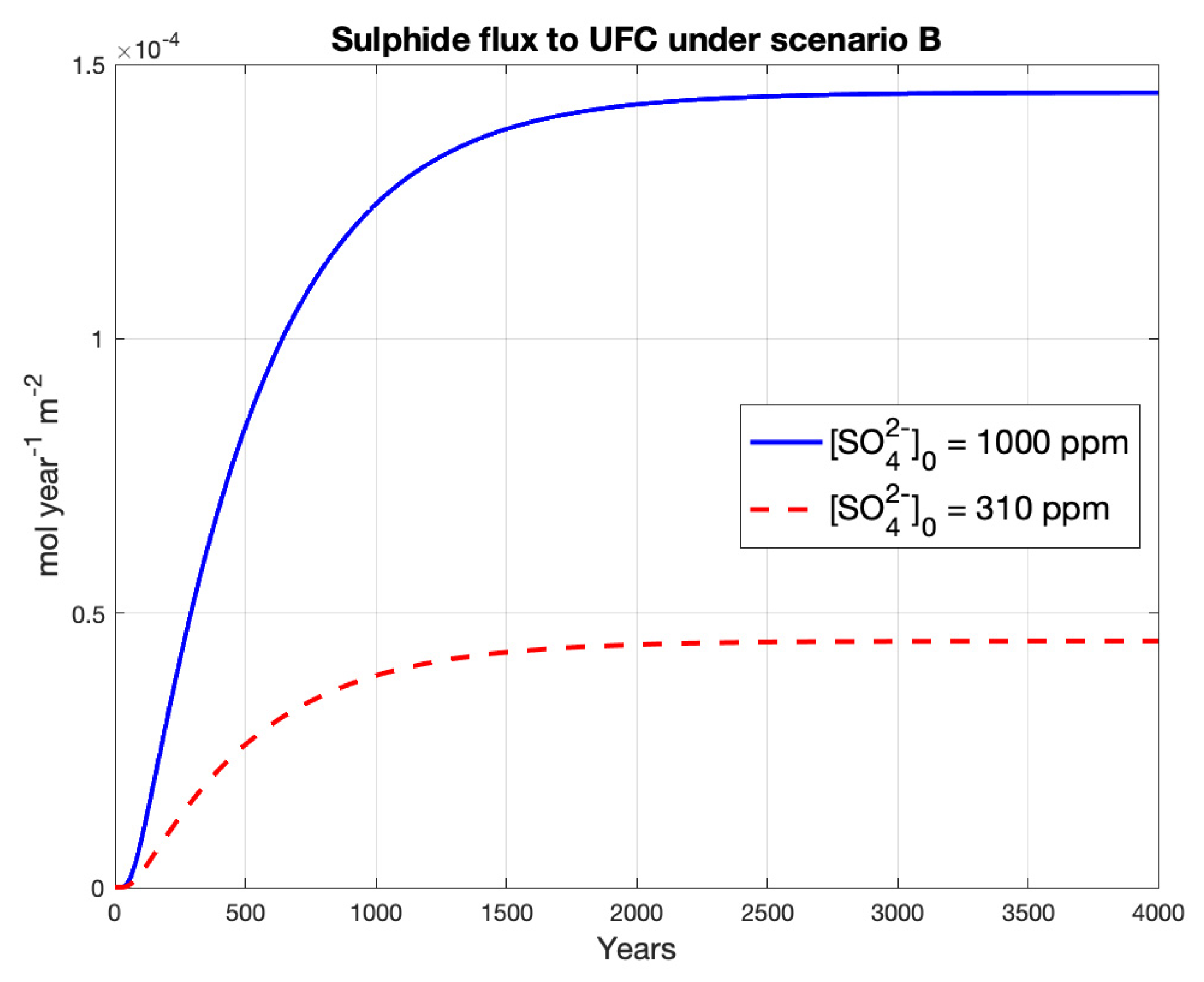
4.2. Scenario B

This scenario, similar to A, has lifetimes above one million years for the deterministic model using both groundwater sulphate concentrations (

Table 6. UFC lifetimes under scenario B [10⁶ years].

		Groundwater Sulphate Concentration
Type of model		1000 ppm	310 ppm
Deterministic lifetime		1.45	4.69
Lognormal draws	Mean	1.49	4.82
	Std. dev.	0.34	1.12
	Minimum	0.63	1.82
	Median	1.45	4.68
	Maximum	3.45	11.6
	Sample	10,000	10,000

). The flux of sulphide to the UFC is slightly higher than the previous scenario, yielding values of approximately 1.4 and 0.4 [mol year⁻¹ m⁻²] for groundwater sulphate concentrations of 1000 and 310 ppm respectively (Figure 4).

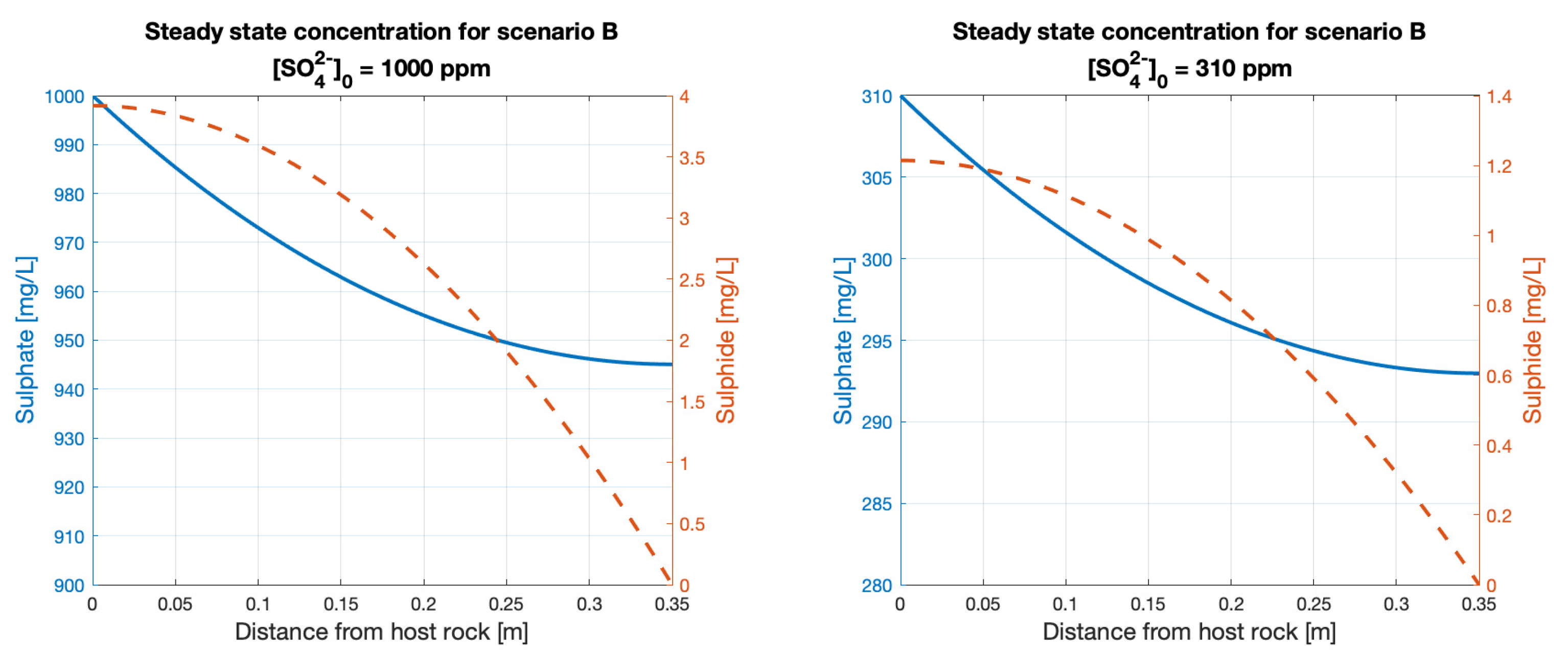
The steady-state sulphide concentrations at the rock interface are similar to those from scenario A, yielding values of approximately 4 and 1.2 ppm of sulphide for the sulphate concentrations of 1000 and 310 ppm respectively (Figure A4 in Appendix A). Unlike scenario A, here the profile of sulphide concentration at a steady-state decreases nonlinearly as it reaches the UFC.

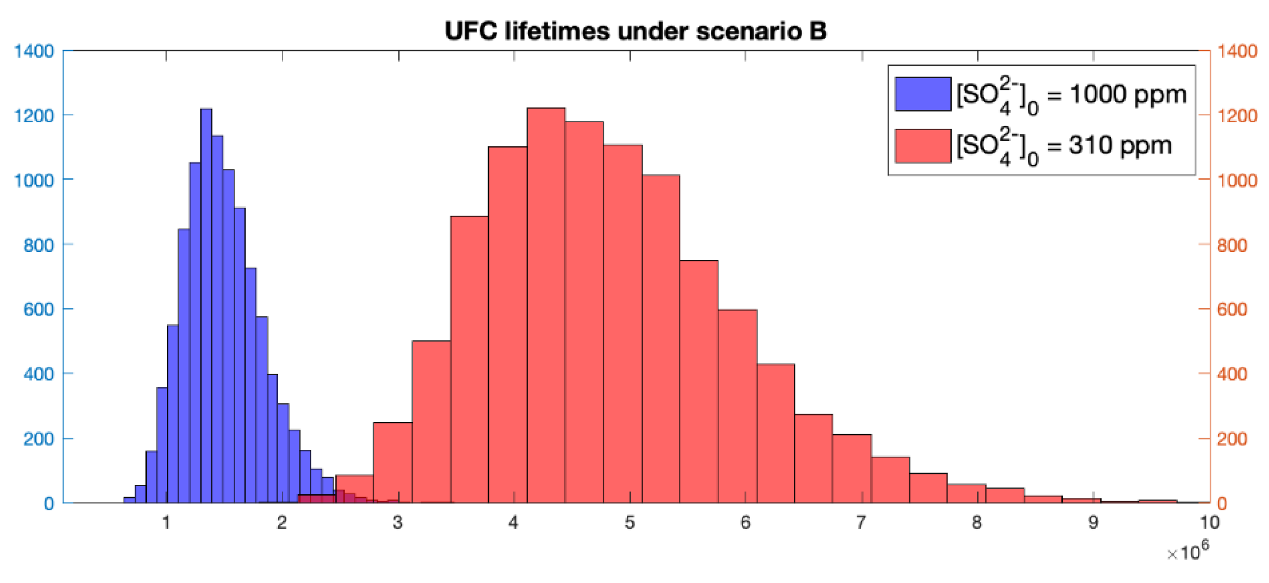
The mean and medium lifetimes values are above one million years for the stochastic model. However, for the higher sulphate concentration simulation, lower than one-million-year lifetimes are possible. The minimum lifetime sampled is around 630,000 years and because the following relation is observed in the results: $Lifetim{e}_{1000ppm}\ast 1000=Lifetim{e}_{310ppm}\ast 310$, the sulphate concentration necessary to yield this minimum lifetime is 2300 ppm, which is an unlikely high value. A histogram of lifetimes of the UFCs for this scenario is shown in Figure 5.

5. Sensitivity Analysis

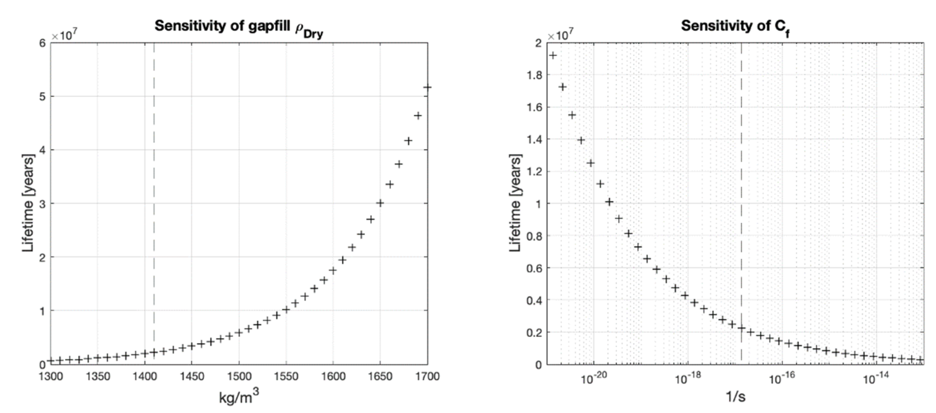
A sensitivity analysis is performed on the dry density of the gapfill bentonite and the optimal parameter $C_f$ of Equation (10). These parameters are selected because they encompass a level of uncertainty and their true value has a significant effect on the lifetimes of the UFCs.

The gapfill bentonite is the material directly in contact to the host rock; therefore, its dry density determines the reduction rate at the rock interface and the mass transport to the HCB buffer box. For scenario A, the gapfill dry density is allowed to vary from 1300 to 1700 [kg/m³] and the density of the HCB is kept at the design value of 1700 [kg/m³]. Since scenario B assumes a uniform density throughout the gapfill and HCB, for this scenario the density of both materials is changed jointly following the range from 1300 to 2000 [kg/m³].

The $C_f$ parameter, which controls the sulphate reduction inside of the bentonite clays (gapfill and HCB), is allowed to vary from four orders of magnitude lower to four orders of magnitude higher than its optimal value.

The highest concentration of sulphate (1000 ppm) is used as a baseline value for these experiments.

6. Discussion and Conclusions

This analysis, the first of its kind on the Canadian deep geological repository (DGR) design, has concentrated on the production of sulphide due to sulphate-reducing bacteria (SRB) activity and the subsequent effect on the time to failure or lifetime of the used fuel containers (UFCs). A first-order kinetics was approximated to describe the reduction of sulphate into sulphide carried out by the SRB. The reaction rate constant is then exponentially adjusted to reflect the high-pressure conditions inside the DGR. The two scenarios created yielded similar sulphide fluxes to the UFC and their lifetimes are above one million years.

The concentration of sulphide at the LHS boundary eventually reaches a steady-state value of between 1 and 4 ppm in both scenarios. This result is in agreement and supports previous studies that have assumed a constant sulphide concentration of 3 ppm [6].

Lifetimes of UFC are inversely proportional to the groundwater sulphate concentration in both scenarios. This relation is expected for scenario A which may, roughly speaking, be characterized as a diffusion system with a source term at the LHS boundary because its steady-state determines the rate of corrosion. However, this relation is somewhat unexpected for scenario B which has a source term throughout the bentonite clay.

Despite that the scenarios entail different assumptions on the behavior of SRB, their results are of the same order of magnitude, which bounds the uncertainty of the effect of having active SRB inside the DGR under the conditions tested. The assumption for scenario A is that SRB would be active only at the rock interface and the region closest to it. While scenario B assumes a more conservative situation, namely, that bacterial activity would be present across the bentonite layers. In both cases, the suppressing effect of high-density bentonite significantly reduces the mass transport of sulphide and corrosion to the UFCs.

The sensitivity analysis shows that more important than the true groundwater chemical concentration of corrosive species, the dry density of the gapfill bentonite or the HCB has a much more significant impact on the mean lifetime of the nuclear waste containers (Figure 6 and Figure 7).

Equally significant is an adequate description of the SRB activity at the walls of the emplacement rooms and inside the bentonite clay. The sensitivity analysis on the parameter $C_f$, that controls the sulphide production inside the bentonite clays, shows that lifetimes are quite sensitive to changes in this value. However, in order to have a more accurate description of the sulphide production, additional experiments on microbial growth and sulphide production would be needed, but this is hindered by the fact that carrying out these physical experiments takes months or longer periods of time. Equally important is the characterization of the rock type, groundwater, and microbial communities of the prospective location of the DGR so that the modeling parameters reflect the particularities of the chosen site.

Future work will focus on including temperature-dependent coefficients to account for the effect of the thermal energy output coming from the UFCs.

References

- Nuclear Waste Management Organization. Postclosure Safety Assessment of a Used Fuel Repository in Crystalline Rock -NWMO TR-2017-02; Nuclear Waste Management Organization: Toronto, ON, Canada, 2017. [Google Scholar]
- Oy, P. Safety Case Plan for the Operating License Application; POSIVA: Eurajoki, Finland, 2017; ISBN 978-951-652-266-4. [Google Scholar]
- SKB. Environmental Impact Statement; SKB: Stockholm, Sweden, 2011. [Google Scholar]
- Noronha, J. Deep Geological Repository Conceptual Design Report Crystalline/Sedimentary Rock Environment-APM-REP-00440-0015 R001; Nuclear Waste Management Organization: Toronto, ON, Canada, 2016. [Google Scholar]
- Nuclear Waste Management Organization. Description of a Deep Geological Repository and Centre of Expertise for Canada’s Used Fuel Container; Nuclear Waste Management Organization: Toronto, ON, Canada, 2015. [Google Scholar]
- Briggs, S.; McKelvie, J.; Sleep, B.; Krol, M. Multi-dimensional transport modelling of corrosive agents through a bentonite buffer in a Canadian deep geological repository. Sci. Total Environ. 2017, 599, 348–354. [Google Scholar] [CrossRef] [PubMed]
- Järvine, A.K.; Murchison, A.G.; Keech, P.G.; Pandey, M.D. A probabilistic model for estimating the life expectancy of used nuclear fuel containers in a Canadian geological repository: Baseline model. Nucl. Eng. Des. 2019, 352, 110202. [Google Scholar] [CrossRef]
- Murakami, H.; Ahn, J. Development of compartment models with Markov-chain processes for radionuclide transport in repository region. Ann. Nucl. Energy 2011, 38, 511–519. [Google Scholar] [CrossRef]
- Marseguerra, M.; Zio, E.; Patelli, E.; Giacobbo, F.; Risoluti, P.; Ventura, G.; Mingrone, G. Modeling the effects of the engineered barriers of a radioactive waste repository by Monte Carlo simulation. Ann. Nucl. Energy 2003, 30, 473–493. [Google Scholar] [CrossRef]
- King, F. Predicting the Lifetimes of Nuclear Waste Containers. JOM 2014, 66, 526–537. [Google Scholar] [CrossRef]
- Nuclear Waste Management Organization. Postclosure Safety Assessment of a Used Fuel Repository in Sedimentary Rock-NWMO TR-2018-08; Nuclear Waste Management Organization: Toronto, ON, Canada, 2018. [Google Scholar]
- Gobien, M.; Garisto, F.; Kremer, E.; Medri, C. Sixth Case Study: Reference Data and Codes-NWMO-TR-2016-10; Nuclear Waste Mangement Organization: Toronto, ON, Canada, 2016. [Google Scholar]
- SKB. Corrosion Calculations Report for the Safety Assessment SR-Site-TR-10-66; SKB: Stockholm, Sweden, 2010; ISBN 1404-0344. [Google Scholar]
- Ochs, M.; Talerico, C. Data and Uncertainty Assessment. Migration Parameters for the Bentonite Buffer in the KBS-3 Concept-SKB-TR-04-18; SKB: Stockholm, Sweden, 2004. [Google Scholar]
- Bengtsson, A.; Blom, A.; Hallbeck, B.; Heed, C.; Johansson, L.; Stahlén, J.; Pedersen, K. Microbial Sulphide-Producing Activity in Water Saturated MX-80, Asha and Calcigel Bentonite at wet Densities from 1500 to 2000 kg m−3; Technical report TR-16-09; SKB: Stockholm, Sweden, 2017; Available online: http://www.skb.com/publication/2487851/TR-16-09.pdf (accessed on 19 August 2021).
- Muyzer, G.; Stams, A.J.M. The ecology and biotechnology of sulphate-reducing bacteria. Nat. Rev. Microbiol. 2008, 6, 441–454. [Google Scholar] [CrossRef] [PubMed]
- Bernardez, L.A.; Lima, L.R.d.; de Jesus, E.B.; Ramos, C.L.; Almeida, P.F. A kinetic study on bacterial sulfate reduction. Bioprocess. Biosyst. Eng. 2013, 36, 1861–1869. [Google Scholar] [CrossRef] [PubMed]
- Huttunen-Saarivirta, E.; Rajala, P.; Carpén, L.I. Corrosion behaviour of copper under biotic and abiotic conditions in anoxic ground water: Electrochemical study. Electrochim. Acta 2016, 203, 350–365. [Google Scholar] [CrossRef]
- Huttunen-Saarivirta, E.; Rajala, P.; Bomberg, M.; Carpén, L. Corrosion of copper in oxygen-deficient groundwater with and without deep bedrock micro-organisms: Characterisation of microbial communities and surface processes. Appl. Surf. Sci. 2017, 396, 1044–1057. [Google Scholar] [CrossRef]
- Binns, J.; Nuclear Waste Management Organization Toronto, ON, Canada. Personal communication, 2018.
- Garcia-Hernandez, J.A. Rule Derivation for Agent-Based Models of Complex Systems: Nuclear Waste Management and Road Networks Case Studies. Ph.D. Thesis, University of Waterloo, Waterloo, ON, Canada, 2018. [Google Scholar]
- Bengtsson, A.; Pedersen, K. Microbial sulphide-producing activity in water saturated Wyoming MX-80, Asha and Calcigel bentonites at wet densities from 1500 to 2000 kg m−3. Appl. Clay Sci. 2017, 137, 203–212. [Google Scholar] [CrossRef]