An Insightful Overview of the Wiener Filter for System Identification

Abstract

Efficiently solving a system identification problem represents an important step in numerous important applications. In this framework, some of the most popular solutions rely on the Wiener filter, which is widely used in practice. Moreover, it also represents a benchmark for other related optimization problems. In this paper, new insights into the regularization of the Wiener filter are provided, which is a must in real-world scenarios. A proper regularization technique is of great importance, especially in challenging conditions, e.g., when operating in noisy environments and/or when only a low quantity of data is available for the estimation of the statistics. Different regularization methods are investigated in this paper, including several new solutions that fit very well for the identification of sparse and low-rank systems. Experimental results support the theoretical developments and indicate the efficiency of the proposed techniques.

1. Introduction

The Wiener filter has been an extremely useful tool since its invention by Norbert Wiener [1]. It represents one of the most popular solutions for system identification problems and finds important applications within a wide range of domains [2,3,4,5]. Basically, the Wiener filter is able to estimate a reference (or desired) random process by filtering an observed noisy process, which is somehow related (or correlated) to the reference signal. In this framework, the filtering process is linear and time invariant, all the signals (input, reference, and noise) are considered stationary processes, and the external (additive) noise that usually corrupts the reference signal is uncorrelated with the input signal. Overall, the Wiener filter is a statistical-based approach, where the solution results following an optimization criterion that relies on the minimization of the mean-squared error. In this context, the error is defined as the difference between the reference signal and the output of the filter.

The optimal solution (i.e., the optimal coefficients) corresponding to the Wiener filter can be simply found by solving a linear system of L equations, where L denotes the length of the impulse response. In other words, the vector (of length L) containing the optimal coefficients is obtained by multiplying the inverse of the covariance matrix of the input signal (of size $L\times L$) with the cross-correlation vector (of length L) between the input and reference signals.

Despite this straightforward mathematical formulation, there are several major challenges related to the use of the Wiener filter in real-world applications. First, the accuracy of the conventional Wiener solution relies on the accuracy of the statistical estimates—namely, the covariance matrix and the cross-correlation vector mentioned previously. In order to reliably estimate these statistics, a large number of data samples (i.e., much larger than L) should be available. However, this is not always the case in practice, since in many applications, a low quantity of data is available, or there is incomplete information about the system. This challenge becomes even more apparent when facing the identification of long-length impulse responses. Second, the matrix inversion operation is also a critical step that should be carefully handled [6]. The basic idea is to avoid an ill-conditioning or a rank-deficient problem, which could result in a bad matrix inversion. For this purpose, the covariance matrix of the input signal needs to be regularized before inversion, usually by adding a positive constant to its main diagonal. It is known that the value of this regularization parameter becomes important in noisy conditions [7]. In other words, the additive noise that usually corrupts the reference signal could significantly influence the overall performance of the Wiener filter, especially in heavy noise environments.

The accuracy of the statistical estimates depends on specific constraints of particular applications, in terms of the availability of the quantity of data. Nevertheless, reformulating a conventional system identification problem using smaller data structures represents a potential solution to improve the behavior of the Wiener filter when dealing with a small quantity of data [8]. In addition, the matrix inversion operation could be avoided by using alternative coordinate descent methods [9]. However, the problem of handling an ill-conditioned matrix remains a critical issue, which can be addressed in terms of using a proper regularization technique, as mentioned before.

The previously mentioned challenges related to the Wiener filter have been addressed in the context of different applications. Recently, in [10], the Kronecker product decomposition of the impulse response was exploited in order to improve the accuracy of the Wiener filter for long-length impulse responses identification. Due to this feature, the resulting solution fits very well in the framework of echo cancellation, for example. In addition, several regularization methods were developed for denoising applications and image restoration, e.g., [11,12,13] and the references therein. Nevertheless, there is still room for performance improvement, especially when using the Wiener filter in challenging conditions, as explained above.

The goal of this paper is to provide new insights into the Wiener filter for system identification problems. The main focus concerns the important practical aspects related to the regularization of this optimal filter in difficult conditions, e.g., working in noisy environments and/or handling a limited set of available data/information. Following this introduction, Section 2 and Section 3 briefly present the system model behind the conventional Wiener filter and some useful background, respectively. Next, Section 4 details different regularization methods of the Wiener filter, also showing how the sparse character of the system can be exploited in this context. Furthermore, a solution obtained using the Kronecker product decomposition of the impulse response is developed in Section 5, which is suitable for low-rank systems identification. In Section 6, the quadratic eigenvalue problem is used for the regularization of the Wiener filter, which can be successfully applied when some a priori knowledge on the impulse response is available. All these techniques and theoretical findings are supported by the simulation results provided in Section 7. Finally, the main conclusions are summarized in Section 8.

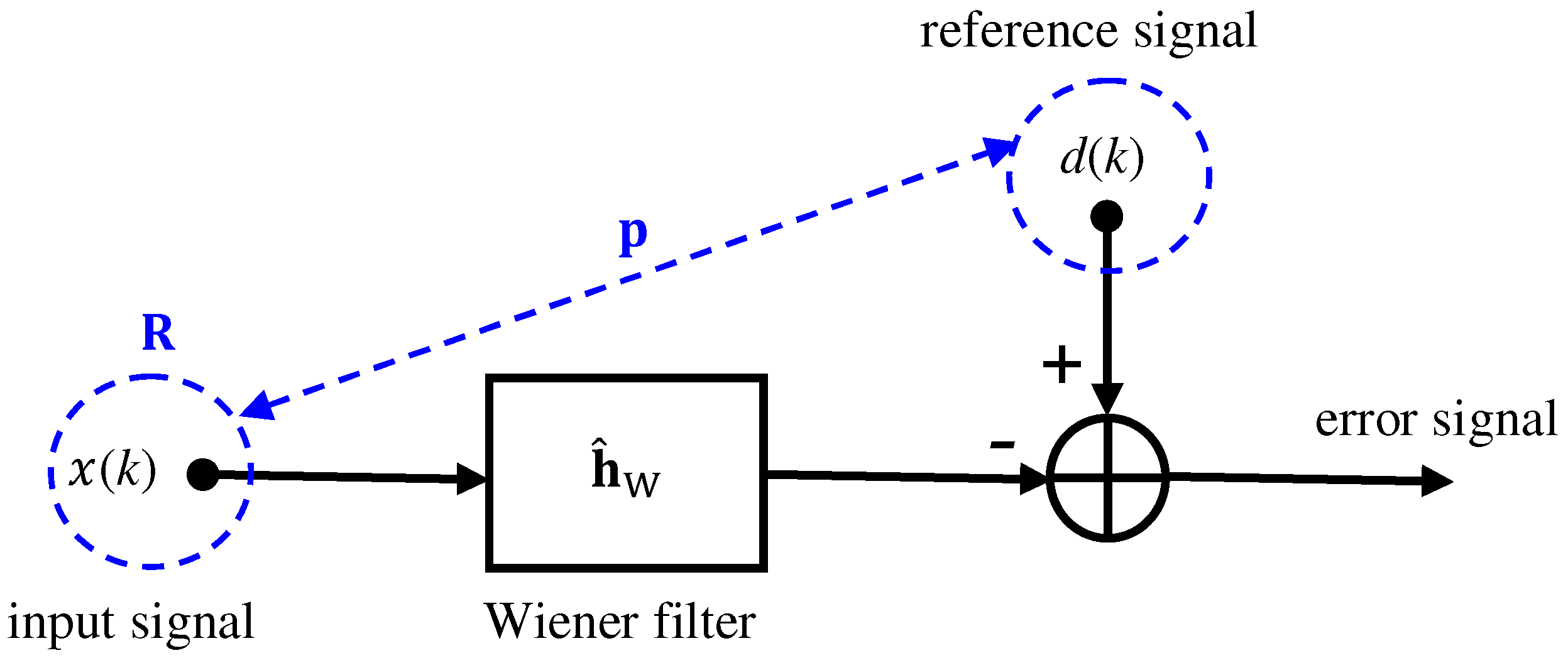
2. System Model and the Conventional Wiener Filter

Let us consider a linear single-input/single-output (SISO) system [14], whose output at the discrete-time index k is given by

$$\begin{array}{cc}\hfill d\left(k\right)& ={\mathbf{h}}^T\mathbf{x}\left(k\right)+w\left(k\right)\hfill \\ \hfill & =y\left(k\right)+w\left(k\right),\hfill \end{array}$$

(1)

where $d\left(k\right)$ is also known as the reference or desired signal,

$$\begin{array}{cc}\hfill \mathbf{x}\left(k\right)& ={\left[\begin{array}{cccc}x\left(k\right)& x(k-1)& \cdots & x(k-L+1)\end{array}\right]}^T\hfill \end{array}$$

is a vector containing the most recent L time samples of the zero-mean input signal $x\left(k\right)$, the superscript ${}^T$ denotes the transpose operator, $\mathbf{h}$ is the unknown system impulse response of length L, and $w\left(k\right)$ is the zero-mean additive noise. It is assumed that the signals take real values and that $x\left(k\right)$ and $w\left(k\right)$ are uncorrelated. Then, the objective of the so-called SISO system identification problem is to identify or estimate $\mathbf{h}$, in the best possible way, given the input signal vector, $\mathbf{x}\left(k\right)$, and the output signal, $d\left(k\right)$. For this purpose, the celebrated Wiener technique is the most appropriate [15,16,17].

From (1), it is clear that the variance of $d\left(k\right)$ is

$$\begin{array}{cc}\hfill {\sigma }_d^2& ={\mathbf{h}}^T\mathbf{R}\mathbf{h}+{\sigma }_w^2,\hfill \end{array}$$

(2)

where $\mathbf{R}=E\left[\mathrm{x}\left(k\right){\mathrm{x}}^T\left(k\right)\right]$ is the $L\times L$ covariance matrix of $\mathrm{x}\left(k\right)$, with $E[·]$ denoting mathematical expectation, and ${\sigma }_w^2$ is the variance of $w\left(k\right)$. It can be deduced from (2) that the signal-to-noise ratio (SNR) of the studied SISO system as presented in (1) is

$$\begin{array}{cc}\hfill \mathrm{SNR}\left(\mathbf{h}\right)& =\frac{{\mathbf{h}}^T\mathbf{R}\mathbf{h}}{{\sigma }_w^2}.\hfill \end{array}$$

(3)

Even though this SNR depends explicitly on the channel impulse response of the system, in many practical identification problems, this SNR is roughly known even if $\mathbf{h}$ is not available [18].

Let $\widehat{\mathbf{h}}$ be a real-valued linear filter of length L, which is also an estimate of $\mathbf{h}$, so that $\widehat{y}\left(k\right)={\widehat{\mathbf{h}}}^T\mathbf{x}\left(k\right)$ is an estimate of $d\left(k\right)$. Then, from the minimization of the popular mean-squared error (MSE) criterion

$$\begin{array}{cc}\hfill \mathcal{J}\left(\widehat{\mathbf{h}}\right)& =E\left\{{\left[d\left(k\right)-{\widehat{\mathbf{h}}}^T\mathbf{x}\left(k\right)\right]}^2\right\}\hfill \\ \hfill & ={\sigma }_d^2-2{\widehat{\mathbf{h}}}^T\mathbf{p}+{\widehat{\mathbf{h}}}^T\mathbf{R}\widehat{\mathbf{h}},\hfill \end{array}$$

(4)

the conventional Wiener filter [3,5] is found

$$\begin{array}{cc}\hfill {\widehat{\mathbf{h}}}_{\mathrm{W}}& ={\mathbf{R}}^{-1}\mathbf{p},\hfill \end{array}$$

(5)

where $\mathbf{p}=E\left[\mathbf{x}\left(k\right)d\left(k\right)\right]$ represents the cross-correlation vector (of length L) between $\mathbf{x}\left(k\right)$ and $d\left(k\right)$. The block diagram of the conventional Wiener filter is depicted in Figure 1. While ${\widehat{\mathbf{h}}}_{\mathrm{W}}$ leads to satisfactory results in many important applications [18], there is still room for improvement.

It should be outlined that in different real-world applications, the presence of outliers (in the input signal and/or external noises) could bias the MSE criterion and, consequently, the solution from (5). This is due to the fact that the basic theory behind the conventional Wiener filter relies on the assumption of zero-mean and stationary signals. In order to cope with different outliers, the conventional approach should further involve additional control and robustness mechanisms, e.g., see [19] and the references therein. The investigation of such particular cases is beyond the scope of this paper.

3. Useful Definitions

In this section, many definitions that will be useful in the rest of this paper are presented.

Let

$$\begin{array}{cc}\hfill \mathbf{h}& ={\left[\begin{array}{cccc}{h}_1& h_2& \cdots & h_L\end{array}\right]}^T\hfill \end{array}$$

be a real-value vector of length L. The ${\ell }_2$ (or Euclidean) norm can be defined as

$$\begin{array}{cc}\hfill {∥\mathbf{h}∥}_2& =\sqrt{{\mathbf{h}}^T\mathbf{h}}=\sqrt{\sum _{l=1}^L{h}_l^2}.\hfill \end{array}$$

(6)

The ${\ell }_1$ norm is given by

$$\begin{array}{cc}\hfill {∥\mathbf{h}∥}_1& =\sum _{l=1}^L\left|h_l\right|.\hfill \end{array}$$

(7)

Another very useful vector norm is the ${\ell }_0$ norm:

$$\begin{array}{cc}\hfill {∥\mathbf{h}∥}_0& =\mathrm{card}\left\{h_l|h_l\ne 0\right\},\hfill \end{array}$$

(8)

where $\mathrm{card}\left\{·\right\}$ stands for cardinality. In other words, the ${\ell }_0$ norm of $\mathbf{h}$ is simply the number of nonzero elements of $\mathbf{h}$.

Let $\mathbf{H}$ be a rectangular matrix of size $L_1\times L_2$ containing real values, where without loss of generality, it is always assumed that $L_1\ge L_2$. The Frobenius norm of $\mathbf{H}$ is defined as

$$\begin{array}{cc}\hfill {∥\mathbf{H}∥}_{\mathrm{F}}& =\sqrt{\mathrm{tr}\left({\mathbf{H}}^T\mathbf{H}\right)},\hfill \end{array}$$

(9)

where $\mathrm{tr}\left(·\right)$ denotes the trace of a square matrix.

The singular value decomposition (SVD) technique [20] is a very powerful tool that can decompose any matrix $\mathbf{H}$ as

$$\begin{array}{cc}\hfill \mathbf{H}& ={\mathbf{U}}_1\mathrm{\Sigma }{\mathbf{U}}_2^T=\sum _{l=1}^{L_2}{\sigma }_l{\mathbf{u}}_{1,l}{\mathbf{u}}_{2,l}^T,\hfill \end{array}$$

(10)

where ${\mathbf{U}}_1=\left[\begin{array}{cccc}{\mathbf{u}}_{1,1}& {\mathbf{u}}_{1,2}& \cdots & {\mathbf{u}}_{1,L_1}\end{array}\right]$ and ${\mathbf{U}}_2=\left[\begin{array}{cccc}{\mathbf{u}}_{2,1}& {\mathbf{u}}_{2,2}& \cdots & {\mathbf{u}}_{2,L_2}\end{array}\right]$ are two orthogonal matrices of sizes $L_1\times L_1$ and $L_2\times L_2$, respectively, and $\mathrm{\Sigma }$ is an $L_1\times L_2$ rectangular diagonal matrix having on its main diagonal nonnegative real numbers. The columns of ${\mathbf{U}}_1$ (resp. ${\mathbf{U}}_2$) are known as the left-singular (resp. right-singular) vectors of $\mathbf{H}$, whereas the diagonal entries ${\sigma }_l,l=1,2,\dots ,L_2$ of $\mathrm{\Sigma }$ are called the singular values of $\mathbf{H}$ with ${\sigma }_1\ge {\sigma }_2\ge \cdots \ge {\sigma }_{L_2}\ge 0$. In the case when the rank of $\mathbf{H}$ is equal to $P\le L_2$, i.e., $\mathrm{rank}\left(\mathbf{H}\right)=P$, then this matrix may be decomposed as

$$\begin{array}{cc}\hfill \mathbf{H}& =\sum _{p=1}^P{\sigma }_p{\mathbf{u}}_{1,p}{\mathbf{u}}_{2,p}^T.\hfill \end{array}$$

(11)

From (10), it is deduced that the nuclear norm of $\mathbf{H}$ is

$$\begin{array}{cc}\hfill {∥\mathbf{H}∥}_{*}& =\sum _{l=1}^{L_2}{\sigma }_l=\mathrm{tr}\left(\sqrt{{\mathbf{H}}^T\mathbf{H}}\right).\hfill \end{array}$$

(12)

Let $L=L_1{L}_2$. $\mathbf{h}$ can be decomposed as

$$\begin{array}{cc}\hfill \mathbf{h}& ={\left[\begin{array}{cccc}{\mathbf{s}}_1^T& {\mathbf{s}}_2^T& \cdots & {\mathbf{s}}_{L_2}^T\end{array}\right]}^T,\hfill \end{array}$$

(13)

where ${\mathbf{s}}_l,l=1,2,\dots ,L_2$ are $L_2$ short vectors of length $L_1$ each. As a result, the vector $\mathbf{h}$ of length $L_1{L}_2$ can be transformed into a rectangular matrix of size $L_1\times L_2$:

$$\begin{array}{cc}\hfill \mathbf{H}& =\left[\begin{array}{cccc}{\mathbf{s}}_1& {\mathbf{s}}_2& \cdots & {\mathbf{s}}_{L_2}\end{array}\right].\hfill \end{array}$$

(14)

Therefore, $\mathbf{h}=\mathrm{vec}\left(\mathbf{H}\right)$, where by $\mathrm{vec}\left(·\right)$ it is denoted the vectorization operation, consisting of converting a matrix into a vector. Furthermore, $\mathbf{H}=\mathrm{ivec}\left(\mathbf{h}\right)$, where $\mathrm{ivec}\left(·\right)$ is the inverse of the vectorization operation.

Let $\mathbf{h}$ be the system impulse response of length L. A good measure of the sparseness of $\mathbf{h}$ is [21,22]

$$\begin{array}{cc}\hfill {\xi }_{12}\left(\mathbf{h}\right)& =\frac{L}{L-\sqrt{L}}\left(1-\frac{{\parallel \mathbf{h}\parallel }_1}{\sqrt{L}{\parallel \mathbf{h}\parallel }_2}\right).\hfill \end{array}$$

(15)

The closer ${\xi }_{12}\left(\mathbf{h}\right)$ is to 1, the sparser is $\mathbf{h}$.

Let $\mathbf{h}=\mathrm{vec}\left(\mathbf{H}\right)$ be the system impulse response and $\widehat{\mathbf{h}}=\mathrm{vec}\left(\widehat{\mathbf{H}}\right)$ its estimate. A good way to evaluate how close is $\widehat{\mathbf{h}}=\mathrm{vec}\left(\widehat{\mathbf{H}}\right)$ to $\mathbf{h}=\mathrm{vec}\left(\mathbf{H}\right)$ is via the normalized misalignment,

$$\begin{array}{cc}\hfill \mathcal{M}\left(\widehat{\mathbf{h}}\right)& =\frac{{∥\mathbf{h}-\widehat{\mathbf{h}}∥}_2}{{∥\mathbf{h}∥}_2}\hfill \end{array}$$

(16)

or, equivalently,

$$\begin{array}{cc}\hfill \mathcal{M}\left(\widehat{\mathbf{H}}\right)& =\frac{{∥\mathbf{H}-\widehat{\mathbf{H}}∥}_{\mathrm{F}}}{{∥\mathbf{H}∥}_{\mathrm{F}}}.\hfill \end{array}$$

(17)

Let $\mathcal{C}$ be a convex set. The convex envelope of a function $f:\mathcal{C}\to \mathbb{R}$ is defined as the largest convex function g such that $g\left(x\right)\le f\left(x\right)$ for all $x\in \mathcal{C}$ [23].

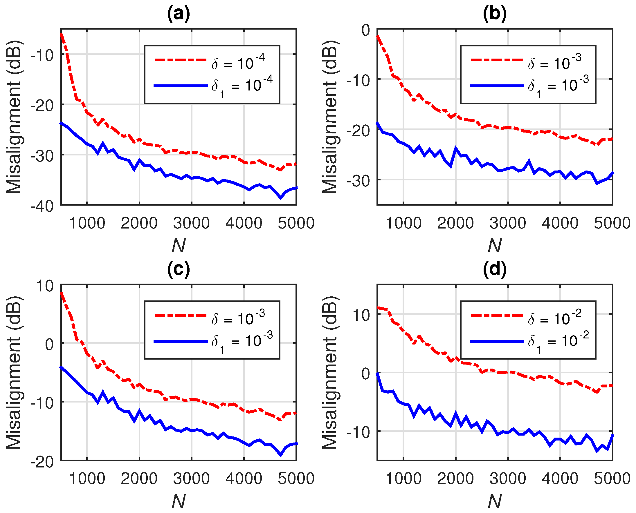
4. Wiener Filter with Different Kinds of Regularization

The Wiener filter can definitely be improved with an appropriate regularization, which should depend on the properties of the system that needs to be identified. In this section, the most useful regularization techniques are exposed.

The most well-known regularization approach is the so-called Tikhonov regularization, which is based on the ${\ell }_2$ norm. The Wiener problem is now

$$\begin{array}{c}\hfill \underset{\widehat{\mathbf{h}}}{min}\left[\mathcal{J}\left(\widehat{\mathbf{h}}\right)+\delta {∥\widehat{\mathbf{h}}∥}_2^2\right],\end{array}$$

(18)

where $\delta \ge 0$ is the regularization parameter, which controls the tradeoff between the fidelity of the original data and large values of the coefficients of the filter. The optimization problem in (18) has obviously a closed-form solution, which is

$$\begin{array}{cc}\hfill {\widehat{\mathbf{h}}}_{\mathrm{W},\delta }& ={\left(\mathbf{R}+\delta {\mathbf{I}}_L\right)}^{-1}\mathbf{p},\hfill \end{array}$$

(19)

where ${\mathbf{I}}_L$ is the $L\times L$ identity matrix. The filter ${\widehat{\mathbf{h}}}_{\mathrm{W},\delta }$ is much more reliable than ${\widehat{\mathbf{h}}}_{\mathrm{W}}$, especially when $\mathbf{R}$ is ill conditioned, and $\mathrm{SNR}\left(\mathbf{h}\right)$ is low.

If the system is sparse, the following optimization problem is more appropriate [24]:

$$\begin{array}{c}\hfill \underset{\widehat{\mathbf{h}}}{min}\left[\mathcal{J}\left(\widehat{\mathbf{h}}\right)+2\delta {∥\widehat{\mathbf{h}}∥}_0\right].\end{array}$$

(20)

This problem finds the sparsest solution, but unfortunately, it is NP-hard [24]. Clearly, a large value of $\delta$ leads to a sparse filter. Using the fact that the convex envelop of ${∥\widehat{\mathbf{h}}∥}_0$ is ${∥\widehat{\mathbf{h}}∥}_1$, ${∥\widehat{\mathbf{h}}∥}_0$ can be replaced by ${∥\widehat{\mathbf{h}}∥}_1$ in (20) to obtain

$$\begin{array}{c}\hfill \underset{\widehat{\mathbf{h}}}{min}\left[\mathcal{J}\left(\widehat{\mathbf{h}}\right)+2\delta {∥\widehat{\mathbf{h}}∥}_1\right],\end{array}$$

(21)

which is now a convex problem [25] and is roughly equivalent to (20). The optimization problem in (21) does not have a closed-form solution, but many iterative/adaptive algorithms exist in the literature that converge to the optimal solution, including proportionate-type adaptive filters [22]. The main advantage of (21) is that even if $\mathbf{R}$ is very ill conditioned, or its estimate is performed with a limited number of observations, if the system is sparse, then a better solution than the conventional Wiener filter can be expected.

Taking the gradient of $\mathcal{J}\left(\widehat{\mathbf{h}}\right)+2\delta {∥\widehat{\mathbf{h}}∥}_1$ with respect to $\widehat{\mathbf{h}}$ and equating the result to zero, it can be found that

$$\begin{array}{cc}\hfill -\mathbf{p}+\mathbf{R}\widehat{\mathbf{h}}+\delta {\mathbf{D}}^{-1}\left(\widehat{\mathbf{h}}\right)\widehat{\mathbf{h}}& =0,\hfill \end{array}$$

(22)

where

$$\begin{array}{cc}\hfill \mathbf{D}\left(\widehat{\mathbf{h}}\right)& =\mathrm{diag}\left(\left|{\widehat{h}}_1\right|,\left|{\widehat{h}}_2\right|,\dots ,\left|{\widehat{h}}_L\right|\right)\hfill \end{array}$$

(23)

is a diagonal matrix and ${\widehat{h}}_l,l=1,2,\dots ,L$ are the elements of $\widehat{\mathbf{h}}$. As a result, (22) can be rewritten as

$$\begin{array}{cc}\hfill \widehat{\mathbf{h}}& ={\left[\mathbf{D}\left(\widehat{\mathbf{h}}\right)\mathbf{R}+\delta {\mathbf{I}}_L\right]}^{-1}\mathbf{D}\left(\widehat{\mathbf{h}}\right)\mathbf{p}.\hfill \end{array}$$

(24)

From the previous expression, it is possible to derive a simple iterative algorithm. At iteration 0, one may take

$$\begin{array}{cc}\hfill {\widehat{\mathbf{h}}}^{\left(0\right)}& ={\widehat{\mathbf{h}}}_{\mathrm{W},\delta }.\hfill \end{array}$$

(25)

Then, at iteration i, it can be written

$$\begin{array}{cc}\hfill {\widehat{\mathbf{h}}}^{\left(i\right)}& ={\left[\mathbf{D}\left({\widehat{\mathbf{h}}}^{(i-1)}\right)\mathbf{R}+{\delta }_1{\mathbf{I}}_L\right]}^{-1}\mathbf{D}\left({\widehat{\mathbf{h}}}^{(i-1)}\right)\mathbf{p},\hfill \end{array}$$

(26)

where ${\delta }_1>0$ is a regularization parameter that is not necessarily equal to $\delta$. The iterations continue until convergence.

Let $L=L_1{L}_2$ with $L_1\ge L_2$, so that $\mathbf{H}=\mathrm{ivec}\left(\mathbf{h}\right)$. In the same way, $\widehat{\mathbf{H}}=\mathrm{ivec}\left(\widehat{\mathbf{h}}\right)$. In many applications, $\mathbf{H}$ is far to be a full-column rank matrix and this important information should be somehow exploited. In other words, $\mathbf{H}$ is a low-rank system. Therefore, in the MSE criterion, it makes more sense to apply a regularization based on the rank of $\widehat{\mathbf{H}}$, i.e., [26]

$$\begin{array}{c}\hfill \underset{\widehat{\mathbf{h}}}{min}\left[\mathcal{J}\left(\widehat{\mathbf{h}}\right)+\delta \mathrm{rank}\left(\widehat{\mathbf{H}}\right)\right].\end{array}$$

(27)

Unfortunately, the matrix rank minimization in (27) is NP-hard, in general, due to the combinatorial nature of the function $\mathrm{rank}\left(·\right)$ [26]. Interestingly, when the matrix $\widehat{\mathbf{H}}$ is diagonal, the previous problem reduces to the optimization problem in (20). Consequently, the sparse problem is taken into account in (27). Using the fact that the convex envelop [27] of $\mathrm{rank}\left(\widehat{\mathbf{H}}\right)$ is ${∥\widehat{\mathbf{H}}∥}_{*}$, (27) is roughly equivalent to the optimization problem [26]:

$$\begin{array}{c}\hfill \underset{\widehat{\mathbf{h}}}{min}\left[\mathcal{J}\left(\widehat{\mathbf{h}}\right)+\delta {∥\widehat{\mathbf{H}}∥}_{*}\right].\end{array}$$

(28)

Some iterative algorithms exist to solve this problem, but they do not seem to work well for long impulse responses; furthermore, complexity may be prohibitive since an approximate SVD needs to be computed at each iteration. Recent insights can be found in [28] and the references therein.

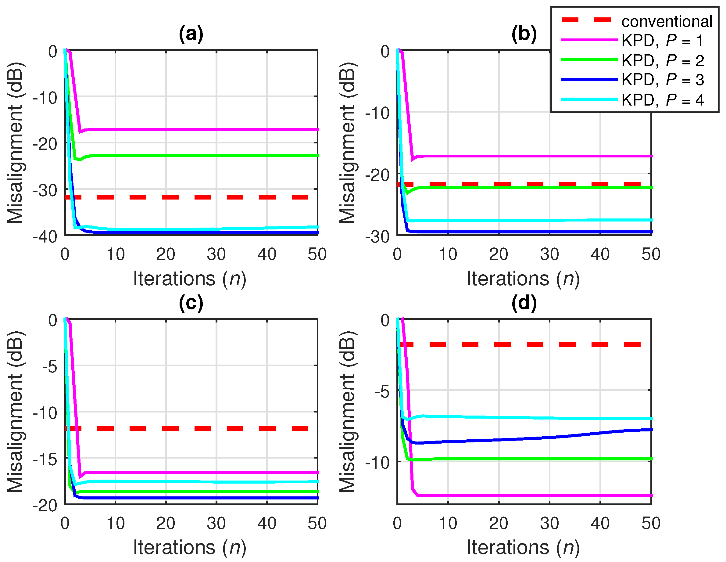
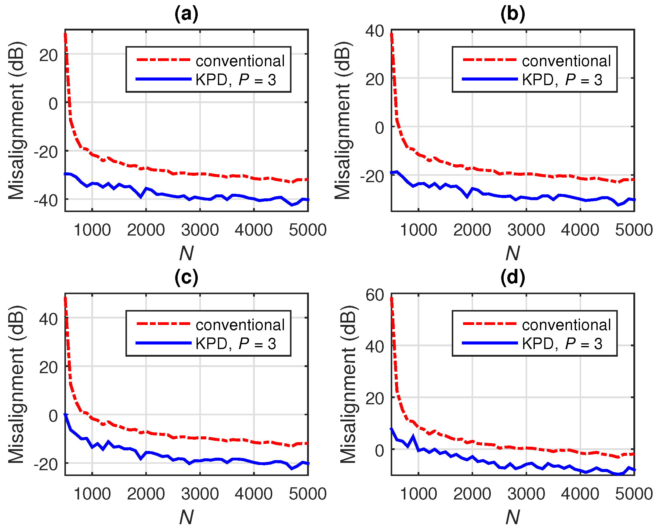
5. Wiener Filter via Kronecker Product Decomposition

In this section, the investigation on the identification of low-rank systems with the Wiener filter is further discussed. An attempt to minimize the nuclear norm of the system in the regularization part was presented in the previous section, but this approach does not seem very practical, and complexity may be extremely high, especially for large matrices.

Here, instead, it is assumed that the rank of the $L_1\times L_2$ matrix $\mathbf{H}$ is known and is much smaller than $L_2$, i.e., $\mathrm{rank}\left(\mathbf{H}\right)=P\ll L_2$. In this case, $\mathbf{H}$ can also be expressed as

$$\begin{array}{cc}\hfill \mathbf{H}& =\sum _{p=1}^P{\mathbf{h}}_{1,p}{\mathbf{h}}_{2,p}^T,\hfill \end{array}$$

(29)

where ${\mathbf{h}}_{1,p}$ and ${\mathbf{h}}_{2,p}$, of lengths $L_1$ and $L_2$, respectively, are impulse responses. This decomposition of $\mathbf{H}$ can be explicitly used in the MSE criterion as explained below. As a result

$$\begin{array}{cc}\hfill \mathbf{h}& =\mathrm{vec}\left(\mathbf{H}\right)\hfill \\ & =\mathrm{vec}\left(\sum _{p=1}^P{\mathbf{h}}_{1,p}{\mathbf{h}}_{2,p}^T\right)\hfill \\ & =\sum _{p=1}^P\mathrm{vec}\left({\mathbf{h}}_{1,p}{\mathbf{h}}_{2,p}^T\right)\hfill \\ & =\sum _{p=1}^P{\mathbf{h}}_{2,p}\otimes {\mathbf{h}}_{1,p},\hfill \end{array}$$

(30)

where ⊗ is the Kronecker product. Furthermore, the filter $\widehat{\mathbf{h}}$ can also be decomposed as

$$\begin{array}{cc}\hfill \widehat{\mathbf{h}}& =\sum _{p=1}^P{\widehat{\mathbf{h}}}_{2,p}\otimes {\widehat{\mathbf{h}}}_{1,p},\hfill \end{array}$$

(31)

where ${\widehat{\mathbf{h}}}_{1,p}$ and ${\widehat{\mathbf{h}}}_{2,p}$ are filters having lengths $L_1$ and $L_2$, respectively. By using the following relationships:

$$\begin{array}{cc}\hfill {\widehat{\mathbf{h}}}_{2,p}\otimes {\widehat{\mathbf{h}}}_{1,p}& =\left({\widehat{\mathbf{h}}}_{2,p}\otimes {\mathbf{I}}_{L_1}\right){\widehat{\mathbf{h}}}_{1,p}\hfill \\ \hfill & =\left({\mathbf{I}}_{L_2}\otimes {\widehat{\mathbf{h}}}_{1,p}\right){\widehat{\mathbf{h}}}_{2,p},\hfill \end{array}$$

(32)

where by ${\mathbf{I}}_{L_1}$ and ${\mathbf{I}}_{L_2}$ are denoted the identity matrices of sizes $L_1\times L_1$ and $L_2\times L_2$, respectively, into (31), it is obtained that

$$\begin{array}{cc}\hfill \widehat{\mathbf{h}}& =\sum _{p=1}^P{\widehat{\mathbf{H}}}_{2,p}{\widehat{\mathbf{h}}}_{1,p}\hfill \\ \hfill & =\sum _{p=1}^P{\widehat{\mathbf{H}}}_{1,p}{\widehat{\mathbf{h}}}_{2,p},\hfill \end{array}$$

(33)

where ${\widehat{\mathbf{H}}}_{2,p}={\widehat{\mathbf{h}}}_{2,p}\otimes {\mathbf{I}}_{L_1}$ and ${\widehat{\mathbf{H}}}_{1,p}={\mathbf{I}}_{L_2}\otimes {\widehat{\mathbf{h}}}_{1,p}$ are matrices of sizes $L_1{L}_2\times L_1$ and $L_1{L}_2\times L_2$, respectively. The two expressions from (33) may be rewritten as

$$\begin{array}{cc}\hfill \widehat{\mathbf{h}}& ={\underline{\widehat{\mathbf{H}}}}_2{\underline{\widehat{\mathbf{h}}}}_1\hfill \\ \hfill & ={\underline{\widehat{\mathbf{H}}}}_1{\underline{\widehat{\mathbf{h}}}}_2,\hfill \end{array}$$

(34)

where

$$\begin{array}{cc}\hfill {\underline{\widehat{\mathbf{H}}}}_2& =\left[\begin{array}{cccc}{\widehat{\mathbf{H}}}_{2,1}& {\widehat{\mathbf{H}}}_{2,2}& \cdots & {\widehat{\mathbf{H}}}_{2,P}\end{array}\right],\hfill \\ \hfill {\underline{\widehat{\mathbf{H}}}}_1& =\left[\begin{array}{cccc}{\widehat{\mathbf{H}}}_{1,1}& {\widehat{\mathbf{H}}}_{1,2}& \cdots & {\widehat{\mathbf{H}}}_{1,P}\end{array}\right]\hfill \end{array}$$

are matrices of sizes $L_1{L}_2\times P{L}_1$ and $L_1{L}_2\times P{L}_2$, respectively, and

$$\begin{array}{cc}\hfill {\underline{\widehat{\mathbf{h}}}}_1& ={\left[\begin{array}{cccc}{\widehat{\mathbf{h}}}_{1,1}^T& {\widehat{\mathbf{h}}}_{1,2}^T& \cdots & {\widehat{\mathbf{h}}}_{1,P}^T\end{array}\right]}^T,\hfill \\ \hfill {\underline{\widehat{\mathbf{h}}}}_2& ={\left[\begin{array}{cccc}{\widehat{\mathbf{h}}}_{2,1}^T& {\widehat{\mathbf{h}}}_{2,2}^T& \cdots & {\widehat{\mathbf{h}}}_{2,P}^T\end{array}\right]}^T\hfill \end{array}$$

are vectors of lengths $P{L}_1$ and $P{L}_2$, respectively. With this Kronecker product decomposition, it can be seen that ${\underline{\widehat{\mathbf{h}}}}_1$ and ${\underline{\widehat{\mathbf{h}}}}_2$ need to be identified instead of $\widehat{\mathbf{h}}$, i.e., $P(L_1+L_2)$ components instead of $L=L_1{L}_2$.

Assume that ${\underline{\widehat{\mathbf{h}}}}_2$ (or, equivalently, ${\underline{\widehat{\mathbf{H}}}}_2$) is fixed. Then, the MSE criterion is

$$\begin{array}{cc}\hfill \mathcal{J}\left({\underline{\widehat{\mathbf{h}}}}_1|{\underline{\widehat{\mathbf{h}}}}_2\right)& =E\left\{{\left[d\left(k\right)-{\underline{\widehat{\mathbf{h}}}}_1^T{\underline{\widehat{\mathbf{H}}}}_2^T\mathbf{x}\left(k\right)\right]}^2\right\}\hfill \\ \hfill & ={\sigma }_d^2-2{\underline{\widehat{\mathbf{h}}}}_1^T{\underline{\mathbf{p}}}_2+{\underline{\widehat{\mathbf{h}}}}_1^T{\underline{\mathbf{R}}}_2{\underline{\widehat{\mathbf{h}}}}_1,\hfill \end{array}$$

(35)

where

$$\begin{array}{cc}\hfill {\underline{\mathbf{p}}}_2& ={\underline{\widehat{\mathbf{H}}}}_2^T\mathbf{p},\hfill \\ \hfill {\underline{\mathbf{R}}}_2& ={\underline{\widehat{\mathbf{H}}}}_2^T\mathbf{R}{\underline{\widehat{\mathbf{H}}}}_2.\hfill \end{array}$$

The minimization of $\mathcal{J}\left({\underline{\widehat{\mathbf{h}}}}_1|{\underline{\widehat{\mathbf{h}}}}_2\right)$ with respect to ${\underline{\widehat{\mathbf{h}}}}_1$ leads to

$$\begin{array}{cc}\hfill {\underline{\widehat{\mathbf{h}}}}_{1,\mathrm{W}}& ={\underline{\mathbf{R}}}_2^{-1}{\underline{\mathbf{p}}}_2.\hfill \end{array}$$

(36)

In the same way, assume that ${\underline{\widehat{\mathbf{h}}}}_1$ (or, equivalently, ${\underline{\widehat{\mathbf{H}}}}_1$) is fixed. Then, the MSE criterion is

$$\begin{array}{cc}\hfill \mathcal{J}\left({\underline{\widehat{\mathbf{h}}}}_2|{\underline{\widehat{\mathbf{h}}}}_1\right)& =E\left\{{\left[d\left(k\right)-{\underline{\widehat{\mathbf{h}}}}_2^T{\underline{\widehat{\mathbf{H}}}}_1^T\mathbf{x}\left(k\right)\right]}^2\right\}\hfill \\ \hfill & ={\sigma }_d^2-2{\underline{\widehat{\mathbf{h}}}}_2^T{\underline{\mathbf{p}}}_1+{\underline{\widehat{\mathbf{h}}}}_2^T{\underline{\mathbf{R}}}_1{\underline{\widehat{\mathbf{h}}}}_2,\hfill \end{array}$$

(37)

where

$$\begin{array}{cc}\hfill {\underline{\mathbf{p}}}_1& ={\underline{\widehat{\mathbf{H}}}}_1^T\mathbf{p},\hfill \\ \hfill {\underline{\mathbf{R}}}_1& ={\underline{\widehat{\mathbf{H}}}}_1^T\mathbf{R}{\underline{\widehat{\mathbf{H}}}}_1.\hfill \end{array}$$

The minimization of $\mathcal{J}\left({\underline{\widehat{\mathbf{h}}}}_2|{\underline{\widehat{\mathbf{h}}}}_1\right)$ with respect to ${\underline{\widehat{\mathbf{h}}}}_2$ leads to

$$\begin{array}{cc}\hfill {\underline{\widehat{\mathbf{h}}}}_{2,\mathrm{W}}& ={\underline{\mathbf{R}}}_1^{-1}{\underline{\mathbf{p}}}_1.\hfill \end{array}$$

(38)

By alternatively iterating between ${\underline{\widehat{\mathbf{h}}}}_{1,\mathrm{W}}$ and ${\underline{\widehat{\mathbf{h}}}}_{2,\mathrm{W}}$, an iterative Wiener filter is obtained, that converges to the true solution [10]. This approach, as shown in [10], performs better than the conventional Wiener filter in various contexts of noise and available data for the estimation of the involved second-order statistics.

A more robust iterative Wiener filter must include regularization based on the ${\ell }_2$ norm, i.e.,

$$\begin{array}{cc}\hfill & \underset{{\underline{\widehat{\mathbf{h}}}}_1}{min}\left[\mathcal{J}\left({\underline{\widehat{\mathbf{h}}}}_1|{\underline{\widehat{\mathbf{h}}}}_2\right)+\delta {\underline{\widehat{\mathbf{h}}}}_1^T{\underline{\widehat{\mathbf{H}}}}_2^T{\underline{\widehat{\mathbf{H}}}}_2{\underline{\widehat{\mathbf{h}}}}_1\right],\hfill \end{array}$$

(39)

$$\begin{array}{cc}\hfill & \underset{{\underline{\widehat{\mathbf{h}}}}_2}{min}\left[\mathcal{J}\left({\underline{\widehat{\mathbf{h}}}}_2|{\underline{\widehat{\mathbf{h}}}}_1\right)+\delta {\underline{\widehat{\mathbf{h}}}}_2^T{\underline{\widehat{\mathbf{H}}}}_1^T{\underline{\widehat{\mathbf{H}}}}_1{\underline{\widehat{\mathbf{h}}}}_2\right],\hfill \end{array}$$

(40)

from which the following optimal solutions are found:

$$\begin{array}{cc}\hfill {\underline{\widehat{\mathbf{h}}}}_{1,\mathrm{W},\delta }& ={\left({\underline{\widehat{\mathbf{H}}}}_2^T\mathbf{R}{\underline{\widehat{\mathbf{H}}}}_2+\delta {\underline{\widehat{\mathbf{H}}}}_2^T{\underline{\widehat{\mathbf{H}}}}_2\right)}^{-1}{\underline{\mathbf{p}}}_2,\hfill \end{array}$$

(41)

$$\begin{array}{cc}\hfill {\underline{\widehat{\mathbf{h}}}}_{2,\mathrm{W},\delta }& ={\left({\underline{\widehat{\mathbf{H}}}}_1^T\mathbf{R}{\underline{\widehat{\mathbf{H}}}}_1+\delta {\underline{\widehat{\mathbf{H}}}}_1^T{\underline{\widehat{\mathbf{H}}}}_1\right)}^{-1}{\underline{\mathbf{p}}}_1,\hfill \end{array}$$

(42)

which is equivalent to regularize the covariance matrix $\mathbf{R}$. Again, by alternatively iterating between ${\underline{\widehat{\mathbf{h}}}}_{1,\mathrm{W},\delta }$ and ${\underline{\widehat{\mathbf{h}}}}_{2,\mathrm{W},\delta }$, a robust iterative Wiener filter is obtained, that converges to the true solution. In order to avoid any potential numerical issues, a very small positive constant should be added to the diagonal of the matrices in (41) and (42) before inversion.

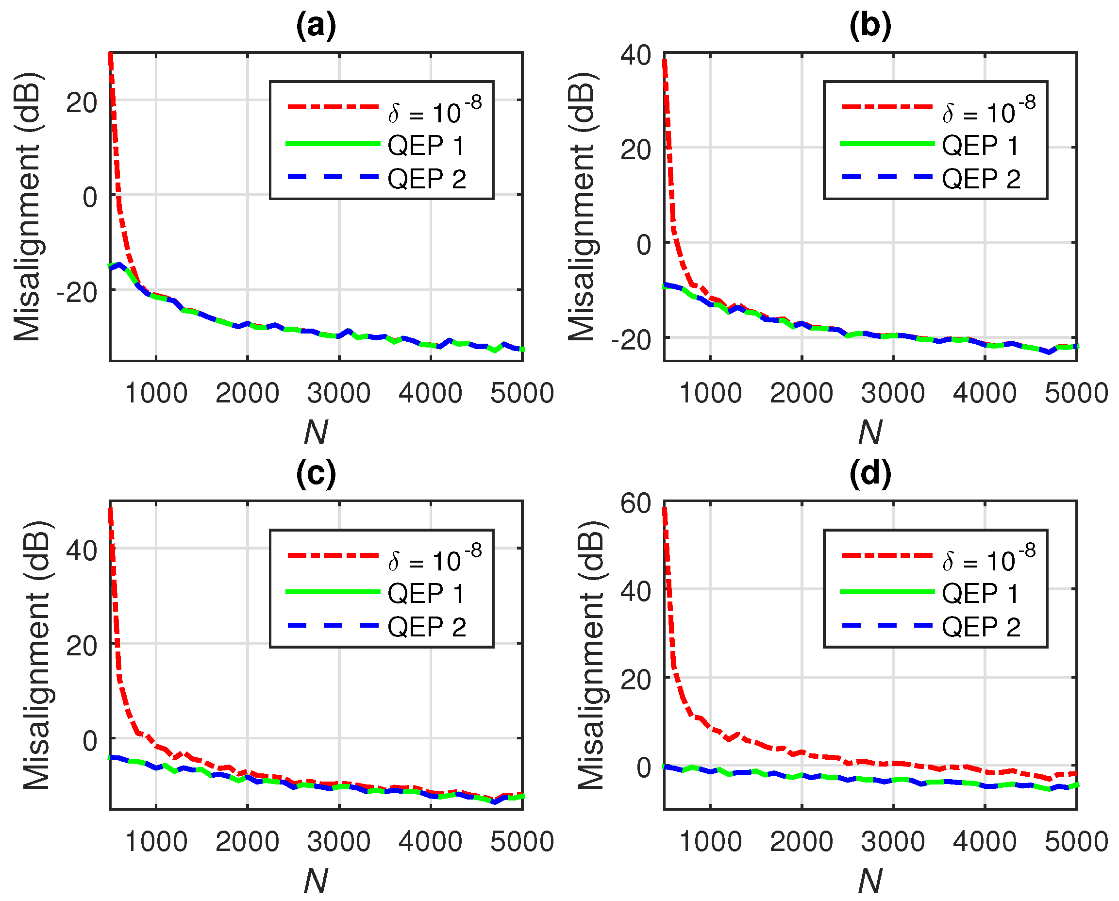
6. Wiener Filter with the Quadratic Eigenvalue Problem

Assume that some knowledge is available on the impulse response, $\mathbf{h}$, i.e., ${∥\mathbf{h}∥}_2^2={\alpha }^2$ with ${\alpha }^2>0$. This information can be used to exactly regularize (with the Tikhonov technique) the Wiener filter with the help of the so-called quadratic eigenvalue problem (QEP) [29,30]. This approach is explained in this section.

The criterion is

$$\begin{array}{c}\hfill \underset{\mathbf{h}}{min}\mathcal{J}\left(\widehat{\mathbf{h}}\right)\mathrm{subject}\mathrm{to}{\widehat{\mathbf{h}}}^T\widehat{\mathbf{h}}={\alpha }^2.\end{array}$$

(43)

From the above criterion, the Lagrange function can be written:

$$\begin{array}{cc}\hfill \mathcal{L}\left(\widehat{\mathbf{h}},\lambda \right)& ={\sigma }_d^2-2{\widehat{\mathbf{h}}}^T\mathbf{p}+{\widehat{\mathbf{h}}}^T\mathbf{R}\widehat{\mathbf{h}}-\lambda \left({\widehat{\mathbf{h}}}^T\widehat{\mathbf{h}}-{\alpha }^2\right),\hfill \end{array}$$

(44)

where $\lambda$ is a Lagrange multiplier. Differentiating $\mathcal{L}\left(\widehat{\mathbf{h}},\lambda \right)$ with respect to $\widehat{\mathbf{h}}$ and $\lambda$ and equating to zero yields the equations:

$$\begin{array}{cc}\hfill \mathbf{R}\widehat{\mathbf{h}}-\lambda \widehat{\mathbf{h}}& =\mathbf{p},\hfill \end{array}$$

(45)

$$\begin{array}{cc}\hfill {\widehat{\mathbf{h}}}^T\widehat{\mathbf{h}}& ={\alpha }^2.\hfill \end{array}$$

(46)

It can be shown [31,32] that the smallest solution $\lambda$ of the two previous equations is needed to solve (43).

Assume that $\lambda$ is not an eigenvalue of $\mathbf{R}$ and let

$$\begin{array}{cc}\hfill \overline{\mathbf{h}}& ={\left(\mathbf{R}-\lambda {\mathbf{I}}_L\right)}^{-1}{\left(\mathbf{R}-\lambda {\mathbf{I}}_L\right)}^{-1}\mathbf{p}\hfill \\ \hfill & ={\left(\mathbf{R}-\lambda {\mathbf{I}}_L\right)}^{-1}\widehat{\mathbf{h}}.\hfill \end{array}$$

(47)

In fact, because $\mathbf{R}>0$, all the eigenvalues of $\mathbf{R}$ are real and strictly positive. To be in accordance with the regularization technique, $\mathbf{R}-\lambda {\mathbf{I}}_L$ also needs to be positive definite. Consequently, $\lambda$ needs to always be negative.

Relations (45) and (46) can be written in terms of $\overline{\mathbf{h}}$ as follows:

$$\begin{array}{cc}\hfill {\left(\mathbf{R}-\lambda {\mathbf{I}}_L\right)}^2\overline{\mathbf{h}}& =\mathbf{p},\hfill \end{array}$$

(48)

$$\begin{array}{cc}\hfill {\overline{\mathbf{h}}}^T{\left(\mathbf{R}-\lambda {\mathbf{I}}_L\right)}^2\overline{\mathbf{h}}& ={\alpha }^2\hfill \\ \hfill & ={\overline{\mathbf{h}}}^T\mathbf{p}.\hfill \end{array}$$

(49)

It is easily deduced from this second equation that

$$\begin{array}{cc}\hfill \frac{{\mathbf{p}}^T\overline{\mathbf{h}}}{{\alpha }^2}& =1.\hfill \end{array}$$

(50)

Developing (48) and using the previous result, it is obtained that

$$\begin{array}{cc}\hfill \left({\mathbf{R}}^2-2\lambda \mathbf{R}+{\lambda }^2{\mathbf{I}}_L\right)\overline{\mathbf{h}}& =\mathbf{p}\hfill \\ \hfill & =\frac{\mathbf{p}{\mathbf{p}}^T}{{\alpha }^2}\overline{\mathbf{h}}.\hfill \end{array}$$

(51)

As a consequence, (51) can be rewritten as

$$\begin{array}{cc}\hfill \left[{\lambda }^2{\mathbf{I}}_L-2\lambda \mathbf{R}+\left({\mathbf{R}}^2-\frac{\mathbf{p}{\mathbf{p}}^T}{{\alpha }^2}\right)\right]\overline{\mathbf{h}}& =0\hfill \end{array}$$

(52)

or alternatively,

$$\begin{array}{cc}\hfill \left({\lambda }^2{\mathbf{A}}_2+\lambda {\mathbf{A}}_1+{\mathbf{A}}_0\right)\overline{\mathbf{h}}& =\mathbf{Q}\left(\lambda \right)\overline{\mathbf{h}}=0,\hfill \end{array}$$

(53)

where

$$\begin{array}{cc}\hfill {\mathbf{A}}_2& ={\mathbf{I}}_L,\hfill \\ \hfill {\mathbf{A}}_1& =-2\mathbf{R},\hfill \\ \hfill {\mathbf{A}}_0& ={\mathbf{R}}^2-\frac{\mathbf{p}{\mathbf{p}}^T}{{\alpha }^2},\hfill \end{array}$$

and $\mathbf{Q}\left(\lambda \right)$ represents the $\lambda$-matrix, which is a degree 2 $L\times L$ matrix polynomial. In (53), the QEP [29] can be recognized, where $\overline{\mathbf{h}}$ is the right eigenvector corresponding to the eigenvalue $\lambda$. Consequently, the solution of (43) is $\widehat{\mathbf{h}}={\left(\mathbf{R}-\lambda {\mathbf{I}}_L\right)}^{-1}\mathbf{p}$, where $\lambda$ is the smallest eigenvalue of (53).

The QEP represents a generalization of the standard eigenvalue problem (SEP), $\mathbf{A}\mathbf{u}=\lambda \mathbf{u}$, and the generalized eigenvalue problem (GEP), $\mathbf{A}\mathbf{u}=\lambda \mathbf{B}\mathbf{u}$. Having a $\lambda$-matrix of size $L\times L$, the QEP has $2L$ eigenvalues (finite or infinite) containing up to $2L$ right and $2L$ left eigenvectors. If there are more than L eigenvectors, then they cannot, of course, be linearly independent [29]. In the current context, since ${\mathbf{A}}_2={\mathbf{I}}_L$ is nonsingular, the QEP has $2L$ finite eigenvalues. Because ${\mathbf{A}}_0$, ${\mathbf{A}}_1$, and ${\mathbf{A}}_2$ are symmetric, the eigenvalues are real or come in pairs $(\lambda ,{\lambda }^{*})$ [29], where the superscript ${}^{*}$ denotes the complex conjugate operator.

An important observation regarding the QEP is that the linearization process is not unique. It is said that a $2L\times 2L$ matrix $\mathbf{A}-\lambda \mathbf{B}$ represents a linearization of the $L\times L$ $\lambda$-matrix $\mathbf{Q}\left(\lambda \right)$ if the eigenvalues of these matrices are identical. Due to this process, the QEP can be solved with the GEP. One option is to take

$$\begin{array}{cc}\hfill \mathbf{A}& =\left[\begin{array}{cc}0& {\mathbf{A}}_0\\ {\mathbf{A}}_0& {\mathbf{A}}_1\end{array}\right],\hfill \end{array}$$

(54)

$$\begin{array}{cc}\hfill \mathbf{B}& =\left[\begin{array}{cc}{\mathbf{A}}_0& 0\\ 0& -{\mathbf{A}}_2\end{array}\right].\hfill \end{array}$$

(55)

It can be checked that if $\mathbf{t}$ is an eigenvector of $\mathbf{Q}\left(\lambda \right)$, then

$$\begin{array}{cc}\hfill \mathbf{u}& =\left[\begin{array}{c}\mathbf{t}\\ \lambda \mathbf{t}\end{array}\right]\hfill \end{array}$$

(56)

is an eigenvector of $\mathbf{A}-\lambda \mathbf{B}$. This process corresponds to the symmetric linearization since both $\mathbf{A}$ and $\mathbf{B}$ are symmetric. The accuracy of this approach will depend on the conditioning of ${\mathbf{A}}_0$ and ${\mathbf{A}}_2$. Another possibility is to take

$$\begin{array}{cc}\hfill \mathbf{A}& =\left[\begin{array}{cc}0& -{\mathbf{I}}_L\\ {\mathbf{A}}_0& {\mathbf{A}}_1\end{array}\right],\hfill \end{array}$$

(57)

$$\begin{array}{cc}\hfill \mathbf{B}& =\left[\begin{array}{cc}-{\mathbf{I}}_L& 0\\ 0& -{\mathbf{A}}_2\end{array}\right]=-{\mathbf{I}}_{2L},\hfill \end{array}$$

(58)

where ${\mathbf{I}}_{2L}$ is the $2L\times 2L$ identity matrix. This linearization is not symmetric. Different linearizations may yield different results; therefore, choosing the right one is important.

The eigenvalues of $\mathbf{Q}\left(\lambda \right)$ can be ordered as

$$\begin{array}{cc}\hfill & \Re \left({\lambda }_1\right)\le \Re \left({\lambda }_2\right)\le \cdots \le \Re \left({\lambda }_{2L}\right),\hfill \end{array}$$

(59)

where $\Re \left(·\right)$ denotes the real part of a complex number. Then, the regularized Wiener filter with the QEP is

$$\begin{array}{cc}\hfill {\widehat{\mathbf{h}}}_{\mathrm{QW}}& ={\left[\mathbf{R}-\Re \left({\lambda }_1\right){\mathbf{I}}_L\right]}^{-1}\mathbf{p}.\hfill \end{array}$$

(60)

Now, if the eigenvalues with the P smallest real parts are considered, another version of the Wiener filter is obtained

$$\begin{array}{cc}\hfill {\widehat{\mathbf{h}}}_{\mathrm{QW},P}& ={\left(\mathbf{R}-{\overline{\lambda }}_P{\mathbf{I}}_L\right)}^{-1}\mathbf{p},\hfill \end{array}$$

(61)

where

$$\begin{array}{cc}\hfill {\overline{\lambda }}_P& =\frac{1}{P}\sum _{p=1}^P\Re \left({\lambda }_p\right).\hfill \end{array}$$

(62)

7. Simulations

In this section, simulation results are provided to support the main theoretical findings related to the regularization of the Wiener filter, which were presented in Section 4, Section 5 and Section 6. All the experiments were performed using MATLAB R2018b on an Asus GL552VX device (Windows 10 OS), having an Intel Core i7-6700HQ CPU @ 2.60 GHz, with 4 Cores, 8 Logical Processors, and 16 GB of RAM.

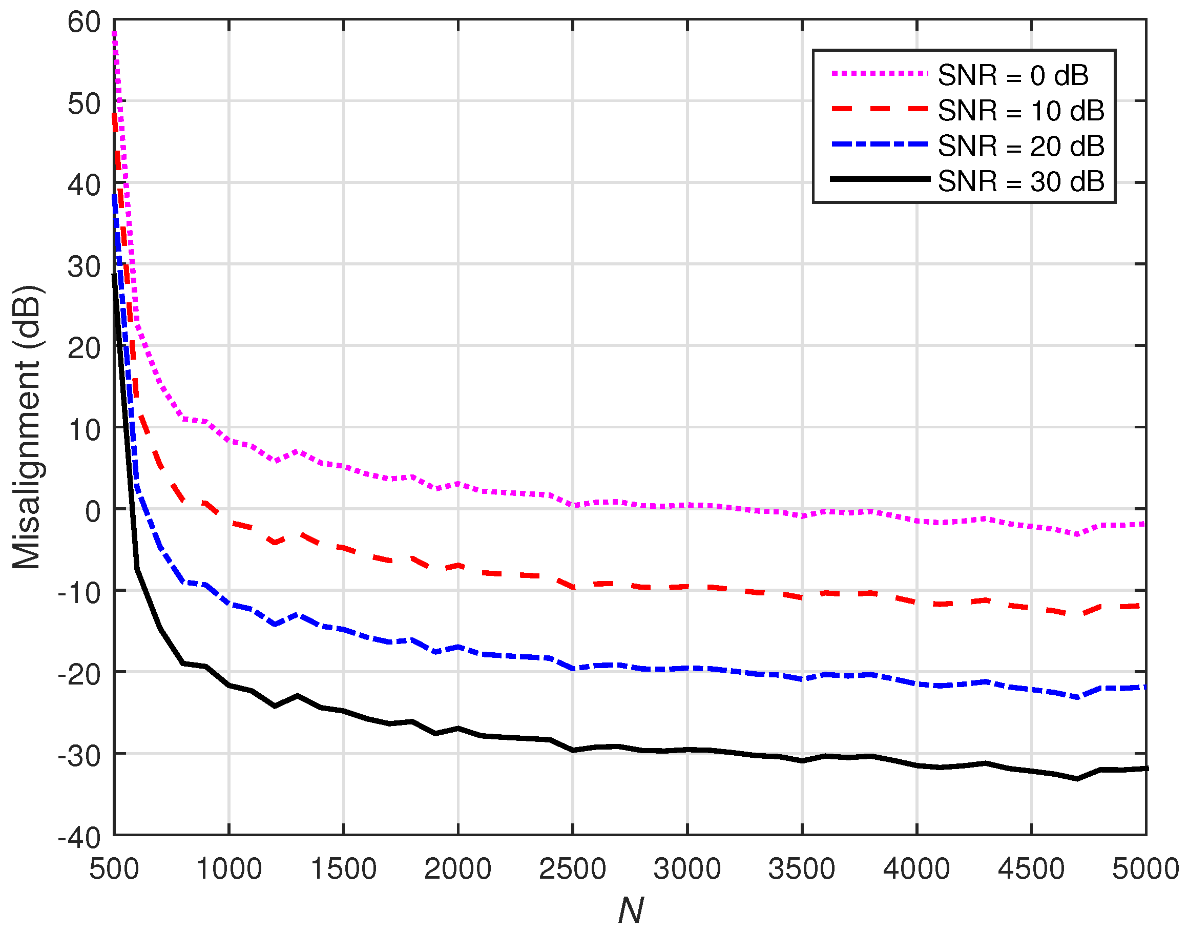
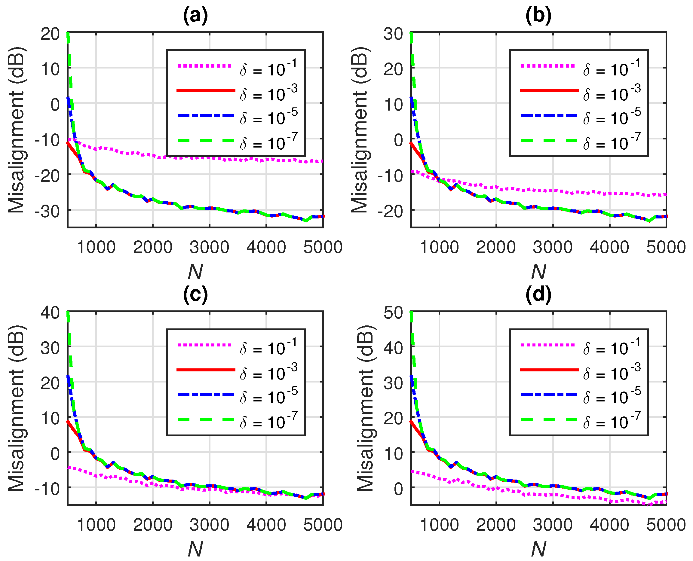
7.1. Conventional Wiener Filter with ${\ell }_2$-Norm Regularization

First, it is important to assess the performance of the conventional Wiener filter, which depends on several important factors, such as the accuracy of the statistical estimates, the SNR, and the regularization parameter. The performance measure is the normalized misalignment (in dB), which is evaluated based on (16). The input signal, $x\left(k\right)$, is an AR(1) process with a pole at 0.9, while the additive noise, $w\left(k\right)$, is white and Gaussian, and different values of the SNR are used. The unknown system, $\mathbf{h}$, is the first impulse response from G168 Recommendation [33], which is padded with zeros up to the length $L=500$. It represents a network echo path, which is sparse in nature. Its sparsity measure can be evaluated based on (15) and results in ${\xi }_{12}\left(\mathbf{h}\right)=0.8957$.

The first critical factor that influences the overall performance of the Wiener filter is the accuracy of the statistical estimates—namely, the covariance matrix, $\mathbf{R}$, and the cross-correlation vector, $\mathbf{p}$. Let us consider that N data samples are used to estimate these quantities, which result in

$$\begin{array}{cc}\hfill \widehat{\mathbf{R}}& =\frac{1}{N}\sum _{k=1}^N\mathbf{x}\left(k\right){\mathbf{x}}^T\left(k\right),\hfill \end{array}$$

(63)

$$\begin{array}{cc}\hfill \widehat{\mathbf{p}}& =\frac{1}{N}\sum _{k=1}^N\mathbf{x}\left(k\right)d\left(k\right).\hfill \end{array}$$

(64)

A higher value of N (as compared to the filter length L) leads to a reliable set of estimates. On the other hand, when a low quantity of data samples is used for the estimation of the statistics (i.e., $N\approx L$), the conventional Wiener filter is not able to provide an accurate solution. Such a scenario is very challenging in different practical applications, where only an incomplete set of data/information is available. Moreover, in the framework of a low SNR environment, the challenges become even more apparent.

In order to highlight these aspects, the performance of the conventional Wiener filter depending on N and for different SNRs is illustrated. Having available the statistical estimates from (63) and (64), the conventional Wiener solution is obtained based on (19). In this simulation, a very small value of the regularization parameter is used, i.e., $\delta ={10}^{-8}$. The results are presented in Figure 2. As expected, a larger value of N improves the Wiener solution, while the accuracy is also influenced by a lower SNR. The critical scenario appears for $N\approx L$, where the conventional Wiener filter is not able to obtain a reliable solution even for a high SNR.

Next, the influence of the regularization parameter, $\delta$, on the performance of the conventional Wiener filter is evaluated in different SNR conditions. First, in Figure 3a,b, good SNR conditions are considered, by setting $\mathrm{SNR}=30$ dB and $\mathrm{SNR}=20$ dB, respectively, while choosing different values for $\delta$. As it can be noticed, the influence of the regularization parameter becomes more apparent when using a low quantity of data (e.g., $N\approx L$) to estimate the statistics. In this case, a larger value of $\delta$ can improve the accuracy of the solution. The influence of the regularization parameter becomes less important for $N\gg L$; in these conditions, a larger value of $\delta$ can even bias the Wiener solution. Nevertheless, in low SNR environments, a larger value of the regularization parameter is required. This is supported in Figure 3c,d, in which the $\mathrm{SNR}$ is set to 10 dB and 0 dB, respectively. As it can be observed, the largest value of $\delta$ improves the performance for any value of N. However, the ${\ell }_2$-norm regularization used in (19) does not exploit the sparse character of the system, which is taken into account within the ${\ell }_1$-norm framework presented in Section 4. Details of these results [focusing on the initial parts of the plots from Figure 3a–d] are shown in Figure 4a–d.

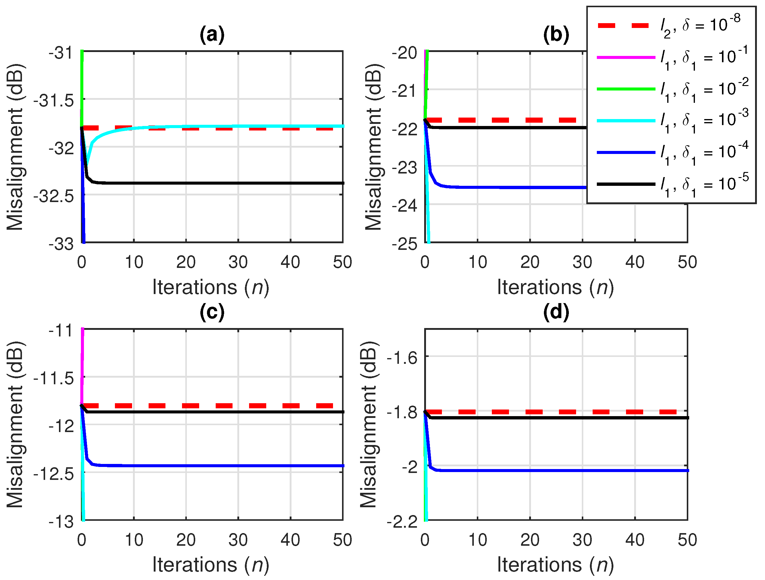
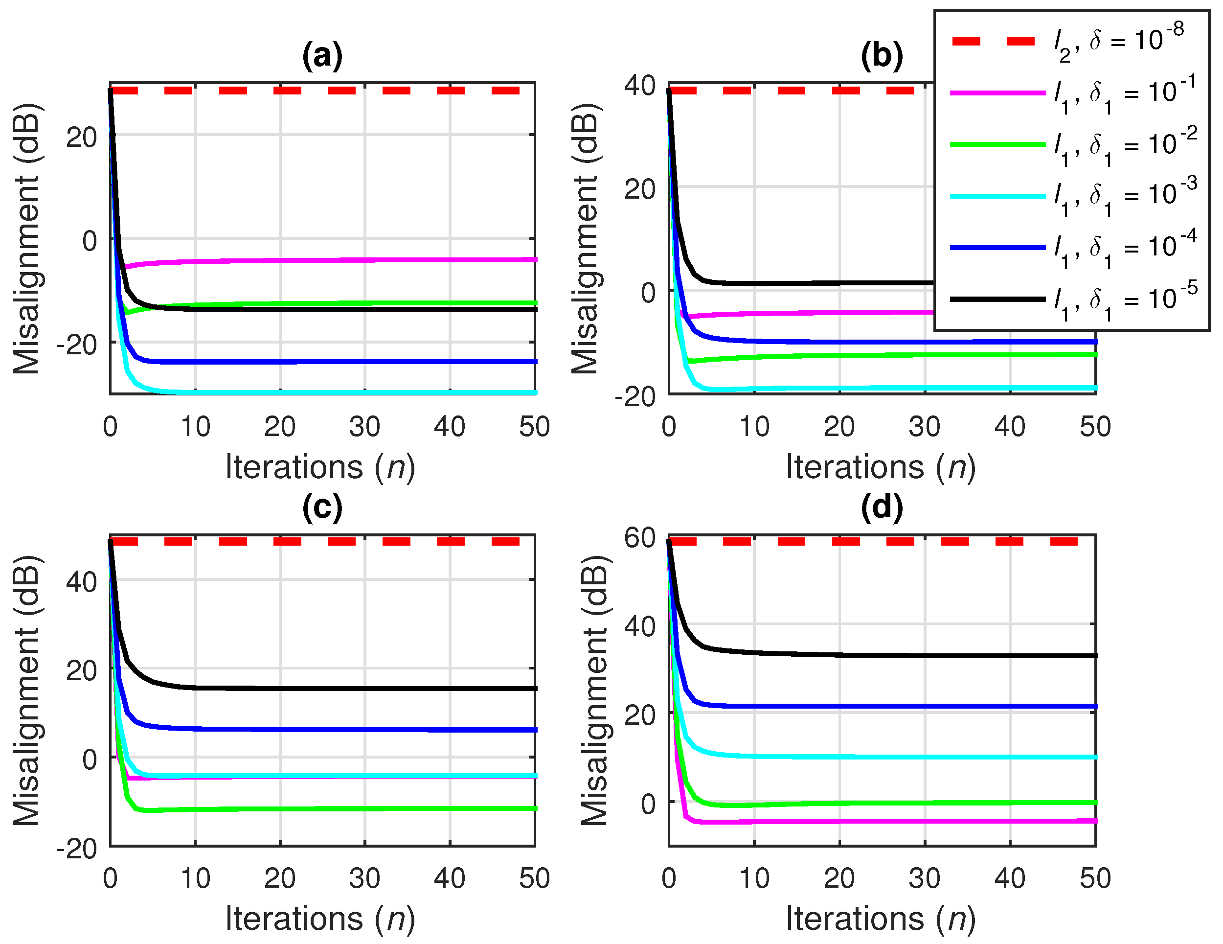
7.2. Iterative Wiener Filter with ${\ell }_1$-Norm Regularization

The iterative ${\ell }_1$-norm regularization from (26) can improve the Wiener solution for sparse system identification. This is supported in the next set of experiments, where the iterative ${\ell }_1$-norm regularization is compared to the conventional ${\ell }_2$-norm regularization of the Wiener filter.

In Figure 5, different $\mathrm{SNRs}$ are set and a large quantity of data is used to estimate the statistics, i.e., $N=5000$. The conventional Wiener filter uses $\delta ={10}^{-8}$, while the iterative ${\ell }_1$-norm regularization involves different values of the parameter ${\delta }_1$ from (26). As it can be observed in Figure 5 (where $N\gg L$), for some values of ${\delta }_1$, the iterative ${\ell }_1$-norm regularization leads to better performance. Details of these results [focusing on the overlapping curves in Figure 5a–d] are shown in Figure 6a–d.

This is more apparent for low values of N, e.g., when $N=L$, as illustrated in Figure 7. In this case, the conventional ${\ell }_2$-norm regularization is clearly outperformed by the iterative ${\ell }_1$-norm version, for all the values of ${\delta }_1$.

The SNR also influences the performance of the iterative ${\ell }_1$-norm regularization, and the values of ${\delta }_1$ from (26) depend on the noise level. As it can be observed in Figure 5, Figure 6 and Figure 7, a higher value of ${\delta }_1$ is required when SNR decreases. On the other hand, the gain of the iterative ${\ell }_1$-norm regularization is more apparent for low SNRs, where it performs much better with respect to the conventional Wiener filter using the ${\ell }_2$-norm regularization.

Finding an optimal value of ${\delta }_1$ is beyond the scope of this paper, in which the main purpose is to outline the features and the potential of the ${\ell }_1$-norm regularization for the identification of sparse systems. However, based on the previous experimental results, some empirical ranges for the values of this parameter could be recommended, depending on the SNR. For example, in good SNR conditions (e.g., $\mathrm{SNR}\ge 20$ dB), a reliable choice could be

$$\begin{array}{cc}\hfill {\delta }_1{|}_{\mathrm{SNR}\left(\mathrm{dB}\right)\ge 20\mathrm{dB}}& ={10}^{-\left(1+{\log }_{10}\mathrm{SNR}\right)}\hfill \\ \hfill & ={10}^{-\left(1+\frac{\mathrm{SNR}\left(\mathrm{dB}\right)}{10}\right)}.\hfill \end{array}$$

(65)

On the other hand, in moderate or low SNR environments (e.g., $0\le \mathrm{SNR}<20$ dB), another option could be

$$\begin{array}{cc}\hfill {\delta }_1{|}_{\mathrm{SNR}\left(\mathrm{dB}\right)<20\mathrm{dB}}& ={10}^{-\left(2+{\log }_{10}\mathrm{SNR}\right)}\hfill \\ \hfill & ={10}^{-\left(2+\frac{\mathrm{SNR}\left(\mathrm{dB}\right)}{10}\right)}.\hfill \end{array}$$

(66)

The validity of these recommended choices are verified in Figure 8, in which the iterative ${\ell }_1$-norm regularization is compared with the conventional ${\ell }_2$-norm regularization in various SNR conditions and for different values of N. Here, $\delta ={\delta }_1$, where ${\delta }_1$ is computed based on (65) and (66), depending on the SNR. As it can be inferred, the iterative ${\ell }_1$-norm regularization works significantly better in all the cases, but its gain is more apparent for low SNRs. Furthermore, the results indicate a good behavior for low values of N, especially for the critical case when $N\approx L$.

7.3. Wiener Filter Based on the Kronecker Product Decomposition

The Wiener filter based on the Kronecker product decomposition (KPD) presented in Section 5 involves smaller data structures with respect to the conventional Wiener filter. While the conventional solution is obtained by directly solving (19), the KPD-based Wiener filter iteratively combines the solutions from (41) and (42). In other words, instead of dealing with a single filter of length $L=L_1{L}_2$ (as in the conventional case), the KPD approach handles two shorter filters of lengths $P{L}_1$ and $P{L}_2$, with $P\ll L_2$. The advantages become more apparent for the identification of long-length impulse responses, such as in echo cancellation [10].

In Figure 9, the conventional Wiener filter is compared with the KPD-based solution using different values of the decomposition parameter P. The regularization parameter is set to $\delta ={10}^{-8}$ for both algorithms. In this simulation, N is set to 5000 and different SNRs are used. As shown in Section 5, the value of P is related to the rank of the matrix $\mathbf{H}$, which reshapes the impulse response $\mathbf{h}$. In this scenario, the length of $\mathbf{h}$ is $L=500$, so that the values $L_1=25$ and $L_2=20$ can be used. In this case, $\mathrm{rank}\left(\mathbf{H}\right)=3$. As it can be observed in Figure 9a–c, the performance of the KPD-based Wiener filter is improved as the value of P increases up to the rank of $\mathbf{H}$. The advantages become more apparent for lower SNRs, where the KPD solution outperforms the conventional Wiener filter for most of the values of P. It is interesting to notice that in heavy noise conditions (e.g., $\mathrm{SNR}=0$ dB), a lower value of P could be used, as indicated in Figure 9d.

In terms of the quantity of data available for the estimation of the statistics, the value $N=5000$ corresponds to a favorable scenario, since $L=500$, so that $N=10L$ in this case. Therefore, a reliable set of statistical estimates [see (63) and (64)] are available. However, even in this favorable scenario, the performance of the conventional Wiener filter is still influenced by the SNR level, as already supported in Figure 2. In other words, the accuracy of its solution is worse when the SNR decreases, as can also be inferred from Figure 9. On the other hand, the KPD-based Wiener filter operates with smaller data structures, and it is less influenced by the accuracy of the statistical estimates, as compared to the conventional Wiener filter. Consequently, it is also more robust to the SNR level. Especially in noisy conditions, i.e., with moderate and low SNRs (e.g., 10 dB and 0 dB, respectively), the KPD-based Wiener filter (for any value of P) outperforms the conventional Wiener solution.

Next, the performance of the KPD-based Wiener filter (using $P=3$) is evaluated for different values of N and in different SNR conditions, using the conventional Wiener filter as a benchmark for comparison. As it can be observed in Figure 10, the KPD approach outperforms the conventional solution for all the values of N and in all SNR conditions. The advantages become more apparent for low values of N, i.e., $N\approx L$.

7.4. Wiener Filter with QEP Regularization

Finally, the last experiment is dedicated to the QEP regularization from (60), which is explained in Section 6. The linearization methods from (54), (55), (57), and (58) are referred in Figure 11 as QEP 1 and QEP 2, respectively. The conventional Wiener filter using $\delta ={10}^{-8}$ is considered for comparison.

In Figure 11, different values of N and different SNRs are used. It can be inferred that the QEP regularization outperforms the regular ${\ell }_2$-norm regularization, especially for low values of N. In heavy noise conditions (e.g., $\mathrm{SNR}=0$ dB), the QEP approach leads to better results for all the values of N, as indicated in Figure 11d. It can also be observed that the two linearization methods perform in a very similar way. It is interesting to compare the results from Figure 11 with the plots from Figure 3. In this context, it can be observed that the QEP regularization is close to the optimal ${\ell }_2$-norm regularization of the Wiener filter.

8. Conclusions

The regularization process is a critical step in any ill-posed problem, especially in noisy environments. This important step is also required in conjunction with the well-known Wiener filter, to avoid an ill-conditioned matrix inversion, as well as to control and improve its performance in low SNR conditions. In this paper, the focus was on several regularization techniques of the Wiener filter.

As shown in Section 4, the classical ${\ell }_2$-norm (or Tikhonov) regularization performs reasonably well only in good or moderate SNR environments. Nevertheless, for sparse systems, the overall performance of the Wiener filter can be improved by using a regularization technique based on the ${\ell }_1$ norm. The iterative solution proposed in this paper outperforms the ${\ell }_2$-norm regularization, especially in challenging conditions, i.e., for low SNRs and/or when using less accurate statistical estimates.

The KPD-based approach is also suitable when only a small quantity of data is available for the estimation of the statistics, as supported in Section 5. The resulting iterative KPD-based Wiener filter can lead to significantly better results, as compared to the conventional Wiener filter for the identification of low-rank systems. This KPD-based version combines the solutions provided by two shorter filters, while the conventional Wiener filter operates with a single filter of much longer length. Consequently, the KPD-based approach fits very well for the identification of long-length impulse responses.

Finally, the QEP regularization technique presented in Section 6 improves the performance of the Wiener filter (as compared to the ${\ell }_2$-norm regularization), especially in noisy environments (i.e., low SNRs), but also when using less accurate estimates of the statistics. Experimental results have supported the main theoretical developments and indicated the robust performance of these regularization techniques.

References

- Wiener, N. Extrapolation, Interpolation, and Smoothing of Stationary Time Series; John Wiley & Sons: New York, NY, USA, 1949. [Google Scholar]
- Ljung, L. System Identification: Theory for the User, 2nd ed.; Prentice-Hall: Upper Saddle River, NJ, USA, 1999. [Google Scholar]
- Haykin, S. Adaptive Filter Theory, 4th ed.; Prentice-Hall: Upper Saddle River, NJ, USA, 2002. [Google Scholar]
- Benesty, J.; Huang, Y. (Eds.) Adaptive Signal Processing—Applications to Real-World Problems; Springer: Berlin, Germany, 2003. [Google Scholar]
- Diniz, P.S.R. Adaptive Filtering: Algorithms and Practical Implementation, 4th ed.; Springer: New York, NY, USA, 2013. [Google Scholar]
- Benesty, J.; Gänsler, T. Computation of the condition number of a nonsingular symmetric Toeplitz matrix with the Levinson–Durbin algorithm. IEEE Trans. Signal Process. 2006, 54, 2362–2364. [Google Scholar] [CrossRef]
- Benesty, J.; Paleologu, C.; Ciochină, S. On regularization in adaptive filtering. IEEE Trans. Audio Speech Lang. Process. 2011, 19, 1734–1742. [Google Scholar] [CrossRef]
- Benesty, J.; Paleologu, C.; Ciochină, S. On the identification of bilinear forms with the Wiener filter. IEEE Signal Process. Lett. 2017, 24, 653–657. [Google Scholar] [CrossRef]
- Zakharov, Y.V.; Tozer, T.C. Multiplication-free iterative algorithm for LS problem. IEE Electron. Lett. 2004, 40, 567–569. [Google Scholar] [CrossRef]
- Paleologu, C.; Benesty, J.; Ciochină, S. Linear system identification based on a Kronecker product decomposition. IEEE ACM Trans. Audio Speech Lang. Process. 2018, 26, 1793–1808. [Google Scholar] [CrossRef]
- Constantin, I.; Richard, C.; Lengellé, R.; Soufflet, L. Nonlinear regularized Wiener filtering with kernels: Application in denoising MEG data corrupted by ECG. IEEE Trans. Signal Process. 2006, 54, 4796–4806. [Google Scholar] [CrossRef]
- Aguena, M.L.S.; Mascarenhas, N.D.A.; Anacleto, J.C.; Fels, S.S. MRI iterative super resolution with Wiener filter regularization. In Proceedings of the XXVI Conference on Graphics, Patterns and Images, Arequipa, Peru, 5–8 August 2013; pp. 155–162. [Google Scholar]
- Li, F.; Lv, X.-G.; Denga, Z. Regularized iterative Weiner filter method for blind image deconvolution. J. Comput. Appl. Math. 2018, 336, 425–438. [Google Scholar] [CrossRef]
- Benesty, J.; Paleologu, C.; Dogariu, L.M.; Ciochină, S. Identification of linear and bilinear systems: A unified study. Electronics 2021, 10, 1790. [Google Scholar] [CrossRef]
- Miller, S.K. Filtering and stochastic control: A historical perspective. IEEE Control Syst. Mag. 1996, 16, 67–76. [Google Scholar]
- Anderson, B.D.O. From Wiener to hidden Markov models. IEEE Control Syst. Mag. 1999, 19, 41–51. [Google Scholar]
- Glentis, G.-O.; Berberidis, K.; Theodoridis, S. Efficient least squares adaptive algorithms for FIR transversal filtering. IEEE Signal Process. Mag. 1999, 16, 13–41. [Google Scholar] [CrossRef]
- Benesty, J.; Sondhi, M.M.; Huang, Y. (Eds.) Springer Handbook of Speech Processing; Springer: Berlin, Germany, 2008. [Google Scholar]
- Pogula, R.; Kumar, T.K.; Albu, F. Robust sparse normalized LMAT algorithms for adaptive system identification under impulsive noise environments. Circuits Syst. Signal Process. 2019, 38, 5103–5134. [Google Scholar] [CrossRef]
- Golub, G.H.; Loan, C.F.V. Matrix Computations, 3rd ed.; The John Hopkins University Press: Baltimore, MD, USA, 1996. [Google Scholar]
- Hoyer, P.O. Non-negative matrix factorization with sparseness constraints. J. Mach. Learn. Res. 2001, 49, 1208–1215. [Google Scholar]
- Paleologu, C.; Benesty, J.; Ciochină, S. Sparse Adaptive Filters for Echo Cancellation; Morgan & Claypool Publishers: San Rafael, CA, USA, 2010. [Google Scholar]
- Hiriart-Urruty, J.B.; Lemaréchal, C. Convex Analysis and Minimization Algorithms II: Advanced Theory and Bundle Methods; Springer: New York, NY, USA, 1993. [Google Scholar]
- Natarajan, B.K. Sparse approximation solutions to linear systems. SIAM J. Comput. 1995, 24, 227–234. [Google Scholar] [CrossRef] [Green Version]
- Donoho, D. Compressed sensing. IEEE Trans. Inf. Theory 2006, 52, 1289–1306. [Google Scholar] [CrossRef]
- Ma, S.; Goldfarb, D.; Chen, L. Fixed point and Bregman iterative methods for matrix rank minimization. Math. Program. Ser. A 2011, 128, 321–353. [Google Scholar] [CrossRef]
- Fazel, M.; Hindi, H.; Boyd, S. A rank minimization heuristic with application to minimum order system approximation. In Proceedings of the American Control Conference, Arlington, VA, USA, 25–27 June 2001; Volume 6, pp. 4734–4739. [Google Scholar]
- Chen, Y.; Chi, Y. Harnessing structures in big data via guaranteed low-rank matrix estimation: Recent theory and fast algorithms via convex and nonconvex optimization. IEEE Signal Process. Mag. 2018, 35, 14–31. [Google Scholar] [CrossRef]
- Tisseur, F.; Meerbergen, K. The quadratic eigenvalue problem. SIAM Rev. 2001, 43, 235–286. [Google Scholar] [CrossRef] [Green Version]
- Chen, X.; Benesty, J.; Huang, G.; Chen, J. On the robustness of the superdirective beamformer. IEEE/ACM Trans. Audio Speech Lang. Process. 2021, 29, 838–849. [Google Scholar] [CrossRef]
- Gander, W. Least squares with a quadratic constraint. Numer. Math. 1981, 36, 291–307. [Google Scholar] [CrossRef]
- Gander, W.; Golub, G.H.; von Matt, U. A constrained eigenvalue problem. Linear Algebra Appl. 1989, 114–115, 815–839. [Google Scholar] [CrossRef] [Green Version]
- Digital Network Echo Cancellers; ITU-T Recommendations G.168; ITU: Geneva, Switzerland, 2002.
Publisher’s Note: MDPI stays neutral with regard to jurisdictional claims in published maps and institutional affiliations. |
© 2021 by the authors. Licensee MDPI, Basel, Switzerland. This article is an open access article distributed under the terms and conditions of the Creative Commons Attribution (CC BY) license (https://creativecommons.org/licenses/by/4.0/).
Share and Cite
Dogariu, L.-M.; Benesty, J.; Paleologu, C.; Ciochină, S. An Insightful Overview of the Wiener Filter for System Identification. Appl. Sci. 2021, 11, 7774. https://doi.org/10.3390/app11177774
Dogariu L-M, Benesty J, Paleologu C, Ciochină S. An Insightful Overview of the Wiener Filter for System Identification. Applied Sciences. 2021; 11(17):7774. https://doi.org/10.3390/app11177774
Chicago/Turabian StyleDogariu, Laura-Maria, Jacob Benesty, Constantin Paleologu, and Silviu Ciochină. 2021. "An Insightful Overview of the Wiener Filter for System Identification" Applied Sciences 11, no. 17: 7774. https://doi.org/10.3390/app11177774
APA StyleDogariu, L.-M., Benesty, J., Paleologu, C., & Ciochină, S. (2021). An Insightful Overview of the Wiener Filter for System Identification. Applied Sciences, 11(17), 7774. https://doi.org/10.3390/app11177774