Article

Low-Complexity Recursive Least-Squares Adaptive Algorithm Based on Tensorial Forms

by
Ionuț-Dorinel Fîciu
,
Cristian-Lucian Stanciu
*,
Cristian Anghel
and
Camelia Elisei-Iliescu
Department of Telecommunications, University Politehnica of Bucharest, 1-3, Iuliu Maniu Blvd., 061071 Bucharest, Romania
*
Author to whom correspondence should be addressed.
Appl. Sci. 2021, 11(18), 8656; https://doi.org/10.3390/app11188656
Submission received: 31 August 2021 / Revised: 14 September 2021 / Accepted: 16 September 2021 / Published: 17 September 2021
(This article belongs to the Special Issue Advance in Digital Signal Processing and Its Implementation)

Abstract

:
Modern solutions for system identification problems employ multilinear forms, which are based on multiple-order tensor decomposition (of rank one). Recently, such a solution was introduced based on the recursive least-squares (RLS) algorithm. Despite their potential for adaptive systems, the classical RLS methods require a prohibitive amount of arithmetic resources and are sometimes prone to numerical stability issues. This paper proposes a new algorithm for multiple-input/single-output (MISO) system identification based on the combination between the exponentially weighted RLS algorithm and the dichotomous descent iterations in order to implement a low-complexity stable solution with performance similar to the classical RLS methods.

1. Introduction

Tensor decomposition is an important topic for the development of modern technologies such as big data, machine learning, communication systems with multiple inputs and/or multiple outputs, respectively source separation/beamforming [1,2,3]. When implementing system identification tasks, the problems can be reformulated to split the arithmetic workload into multiple smaller system identification problems. Considerable recent research was dedicated to identify multilinear forms [4,5,6] with two, three, or even more components using the Wiener filter [7,8,9] and adaptive algorithms based on the least-mean-square (LMS) method [10,11,12,13] or on the recursive least-squares (RLS) systems [10,14,15]. Despite the attractive performance of the latter, its classical implementations are considered too costly for most practical applications and the preferred workhorse remains the LMS or the normalized-LMS (NLMS) method, which is not sensitive to the scaling of its input signal.
The traditional least-squares based adaptive systems require complexities proportional to the second or third power of the filter’s length in order to compute the corresponding matrix inverse and the associated coefficients. The filter update employs a full spectrum of mathematical operations, including divisions, and it is often plagued by numerical instability. Despite its prohibitive nature in terms of required chip area, the decorrelation properties of the RLS (translated in practice into superior convergence speeds and overall performance) pushed researchers to develop new corresponding versions with attractive compromise between complexity and performance. However, for some algorithms, such as Fast-RLS (FRLS) [16], the negative aspects still tend to overtake the value brought by the reduction in terms of complexity and deny the practical applications a reliable least-squares algorithm.
For the system identification implementations, which can be decomposed using multiple-input/single-output (MISO) setups, several tensor based models were recently proposed [11]. One such decomposition uses the RLS method based on Woodburry’s identity [15] to split the unknown system determination into multiple smaller adaptive systems. Despite the fact that the overall complexity is reduced, the algorithm previously introduced as tensor-based RLS (RLS-T) is still dependent on the square of each filter’s length, and it is also prone to inherit the problems of classical least-squares solutions [14].
Recently, amongst the newly proposed RLS methods, the combination with the dichotomous coordinate descent (DCD) iterations has been established as a possible stable alternative with lower complexity traits, proportional to the adaptive filter’s length. This paper proposes a tensorial decomposition for multilinear forms based on the RLS-DCD method, which was extensively studied and widely accepted as an efficient solution for least-squares adaptive systems [17,18]. The DCD portion of the algorithm exploits the nature of the corresponding correlation matrices and estimates with minimal computational effort, in an iterative manner, an incremental vector for each of the adaptive filter to be updated. The operations are performed using only additions and bit-shifts, and any overall requirement for divisions is eliminated [19,20]. For the identification of an unknown MISO system based on its tensorial form, multiple RLS-DCD smaller adaptive filters will be employed, which inherit the performance of the classical RLS versions and require lower arithmetic efforts.
The paper is organized as follows: Section 2 introduces the framework of the multilinear forms. In Section 3, the RLS-T is described with its corresponding notations and the newly RLS-DCD-T adaptive systems are introduced as an alternative for the former. The new adaptive model is validated in Section 4 through several simulation results and conclusions are presented in Section 5.

2. System Model

Considering N individual channels described by the following vectors:
h i = h i , 1 h i , 2 h i , L i T ,
each one of length L i , i = 1 , 2 , , N , where the superscript T denotes the transpose operator, they compose a multiple-input/single-output (MISO) system. For efficiency reasons, in the rest of the paper, the index i will repeatedly have the same significance as the one mentioned for Equation (1) (i.e., to identify elements associated with the i-th channel). Its corresponding real valued output is represented at the discrete-time index n by the expression:
y ( n ) = l 1 = 1 L 1 l 2 = 1 L 2 l N = 1 L N x l 1 l 2 l N ( n ) h 1 , l 1 h 2 , l 2 h N , l N ,
where the input signals from (2) can be aggregated using the tensorial form X ( n ) R L 1 × L 2 × × L N , with the constituent elements X l 1 l 2 l N ( n ) = x l 1 l 2 l N ( n ) . Such linearly separable systems are subject of research for applications like nonlinear acoustic echo cancellation [21,22], beamforming [3,23], or source separation techniques [1,2].
Consequently, the input–output equation can be written as
y ( n ) = X ( n ) × 1 h 1 T × 2 h 2 T × 3 × N h N T ,
where × i is the mode-i product explained in [1], and y ( n ) is a linear function of each of the vectors h i , when the other N 1 vectors are fixed (i.e., y ( n ) connotes a multilinear form). Due to this hypothesis, the structure presented in (2) and (3) can be interpreted as an extension of the bilinear form [24].
Moreover, we denote the tensor H R L 1 × L 2 × × L N , with the elements H l 1 , l 2 , , l N = h 1 , l 1 h 2 , l 2 h N , l N , as the result of:
H = h 1 h 2 h N ,
where ∘ symbolizes the outer product, defined as h 1 h 2 = h 1 h 2 T , with the corresponding elements h 1 h 2 i , j = h 1 , i h 2 , j . At this stage, it is noteworthy that the Kronecker product between two vectors (denoted using ⊗) can be expressed as h 2 h 1 = vec h 1 h 2 , where vec ( · ) is the vectorization operation.
Therefore, we write
vec H = h N h N 1 h 1 ,
and we reformulate the output signal as
y ( n ) = vec T H vec X ( n ) ,
where
vec X ( n ) = vec X : : : 1 ( n ) vec X : : : 2 ( n ) vec X : : : L N ( n ) = x ( n ) ,
with X : : : l i ( n ) R L 1 × L 2 × × L N 1 representing the frontal slices of X ( n ) and x ( n ) denoting the input vector of length L = L 1 L 2 L N . In addition,
g = vec H = h N h N 1 h 1
symbolizes the global impulse response of length L 1 L 2 L N . The decomposition from (8) is not given by a unique set of estimators corresponding to the individual members. Exemplifying, let us consider N real-valued constants c i , having the property that i = 1 N c i = 1 . Then,
c N h N c N 1 h N 1 c 1 h 1 = h N h N 1 h 1 .
Nevertheless, the global impulse response g can be identified with no scaling ambiguity.
Furthermore, considering (6)–(8), y ( n ) can be rewritten as
y ( n ) = g T x ( n ) .
The target is to identify the unknown global system g given by its individual components h i by using the reference signal:
d ( n ) = g T x ( n ) + w ( n ) ,
where the measurement noise, w ( n ) , is uncorrelated with the incoming signal. The reference signal from (11) is described by the variance:
σ d 2 = g T E x ( n ) x T ( n ) g + σ w 2 = g T R g + σ w 2 .
E [ · ] denotes mathematical expectation, R = E x ( n ) x T ( n ) , and σ w 2 = E [ w 2 ( n ) ] .
The error signal has the expression:
e ( n ) = d ( n ) g ^ T x ( n ) ,
where g ^ describes an estimator of the global impulse response.
The Wiener approach for the estimate g ^ [14] is not suitable in nonstationary conditions. Moreover, the requirement of real-time processing makes it only a starting point in providing more adequate solutions based on adaptive algorithms. The majority of adaptive systems rely on the LMS-based methods, which offer a satisfactory balance between performance and arithmetic workload. However, state-of-the-art literature provides several versions of the RLS adaptive filter as appealing alternatives with better performance indicators (i.e., tracking speed, convergence rate). Despite of the advantages which the RLS-based versions have over their LMS-based counterparts, most of the RLS algorithms cannot provide stable functionality combined with proper arithmetic complexity. In recent years, the integration between the dichotomous coordinate descend (DCD) iterative methods [20] with the RLS adaptive filters [14] successfully contested the prohibitive tag associated with the RLS family implementations. The RLS-DCD delivered promising results with acceptable processing requirements and performance similar to the classical RLS versions.
Now, having (13), we can define the mean-squared error (MSE) criterion:
J g ^ = E e 2 ( n ) = σ d 2 2 g ^ T p + g ^ T R g ^ ,
with p = E x ( n ) d ( n ) representing the cross-correlation vector between x ( n ) and d ( n ) . Our focus is the minimization of J g ^ , and it represents the optimization criterion. In order to do this, we may use the well-known solution [14] given by the Wiener filter:
g ^ W = R 1 p .
With the iterative Wiener filter [8], we are able to speculate the decomposition of the global impulse response, considering the topic of the multilinear forms. The optimization criterion consists on a block coordinate descent method applied on the individual components [25]. Comparing to the standard Wiener filter given by Equation (15), the iterative one boosts the performance. It is suitable, especially when a small amount of data are used in order to estimate the statistics of the signal (i.e., R and p ).

3. Tensor-Based RLS Algorithms

The faster convergence rate is one of the main advantages of the RLS methods, with respect to the performances obtained by the LMS-based family of algorithms. However, this convergence aspect comes together with a very high computational complexity. It was previously demonstrated that tensor-based algorithms could produce better results than the classical RLS approach, by splitting the long filter associated with the unknown system identification problem into multiple smaller filters, i.e., into multiple smaller system identification processes. The main advantages of this category of adaptive algorithms are two-fold: a significant decrease in number of mathematical operations and improved convergence rates.

3.1. Tensor-Based Recursive Least Squares Algorithm (RLS-T)

Starting with the desired (11) and error (13) signals, we can apply the least-squares error criterion [14] for the tensor-based decomposition. The RLS algorithm can be applied by following the minimization of the cost function:
J g ^ ( n ) = k = 1 n λ n k d ( k ) g ^ T ( n ) x ( k ) 2 ,
with the forgetting factor of the algorithm, 0 < λ 1 .
First, let us consider the estimated impulse responses of the channels, h ^ i ( n ) . Therefore, we may define the corresponding a-priori error signals:
e h ^ i ( n ) = d ( n ) y h ^ i ( n )
= d ( n ) h ^ i T ( n 1 ) x h ^ i ( n ) ,
where y h ^ i ( n ) are the outputs of the individual channels, and we used the form x ( n ) defined in (7) to express
x h ^ i ( n ) = h ^ N ( n 1 ) h ^ N 1 ( n 1 ) h ^ i + 1 ( n 1 ) I L i h ^ i 1 ( n 1 ) h ^ 2 ( n 1 ) h ^ 1 ( n 1 ) T x ( n ) ,
with I L i denoting the identity matrices of sizes L i × L i . It can be verified that e h ^ 1 ( n ) = e h ^ 2 ( n ) = = e h ^ N ( n ) .
Considering (19), the cost function in (16) can be reworked in N alternative ways by performing the optimization procedure of the individual impulse responses, i.e.,
J h ^ N , h ^ N 1 , , h ^ i + 1 , h ^ i 1 , , h ^ 2 , h ^ 1 h ^ i ( n ) = k = 1 n λ i n k d ( k ) h ^ i T ( n ) x h ^ i ( k ) 2 ,
where the λ i ’s are the individual forgetting factors. These impulse responses can be processed by following a multilinear optimization strategy [25], considering the fact that N 1 components are fixed, and the optimization method is applied to the remaining one. Therefore, the focus is the minimization of (20) with respect to h ^ i ( n ) , which leads to a set of normal equations:
R i ( n ) h ^ i ( n ) = p i ( n ) ,
where
R i ( n ) = k = 1 n λ i n k x h ^ i ( k ) x h ^ i T ( k )
= λ i R i ( n 1 ) + x h ^ i ( n ) x h ^ i T ( n ) ,
p i ( n ) = k = 1 n λ i n k x h ^ i ( k ) d ( k )
= λ i p i ( n 1 ) + x h ^ i ( n ) d ( n ) .
We can achieve N update relations linked to the individual filters by solving Equation (21). The obvious requirement for its corresponding solutions is the computation of the inverse matrices R i ( n ) . The straightforward approach is considered too costly for real-time practical applications. A well-known and accepted compromise, which is often used as a reference, is the method provided by the matrix inversion lemma (also known as Woodbury’s matrix identity) [14]. We can express the inverse matrices as
R i 1 ( n ) = 1 λ i I L i k i ( n ) x h ^ i T ( n ) R i 1 ( n 1 ) ,
where
k i ( n ) = R i 1 ( n 1 ) x h ^ i ( n ) λ i + x h ^ i T ( n ) R i 1 ( n 1 ) x h ^ i ( n )
denotes the Kalman gain vectors.
Consequently, the filter updates can be performed using
h ^ i ( n ) = h ^ i ( n 1 ) + R i 1 ( n ) x h ^ i ( n ) e h ^ i ( n )
= h ^ i ( n 1 ) + k i ( n ) e h ^ i ( n ) ,
where k i ( n ) = R i 1 ( n ) x h ^ i ( n ) are the Kalman gain vectors. The error signal can be easily computed by using (18).
The arithmetic complexity associated with the computation of each set of filter coefficients is proportional to the square of the corresponding filter length. The usage of a single adaptive filter is similarly prohibitive for hardware implementations.
In the end, the estimate of the resulting filter can be obtained using
g ^ ( n ) = h ^ N ( n ) h ^ N 1 ( n ) h ^ 1 ( n ) .
The tensor-based RLS (RLS-T) algorithm is available in Algorithm 1. This approach has been deeply analyzed in the paper [26] by using N = 3 (i.e., third-order tensors). The current sub-section described a generalization for N 3 , thus providing even more efficient implementation solutions based on RLS adaptive filters. However, the RLS-T form requires for each of the N filters a computational workload proportional to L i 2 . When considering applications where one of the filters still has a considerable amount of weights, the cost of practical implementations remains quite high.
Algorithm 1: RLS-T algorithm
    StepActions
Initialization :
      Set h ^ i ( 0 )
    0       R i 1 ( 0 ) = δ i 1 I L i , δ i > 0
       λ i = 1 1 K i L i , K i 1
For n = 1 , 2 , , number of iterations :
    1      Compute x h ^ i ( n ) , based on (19)
    2       e h ^ i ( n ) = d ( n ) h ^ i T ( n 1 ) x h ^ i ( n )
    3       k i ( n ) = R i 1 ( n 1 ) x h ^ i ( n ) λ i + x h ^ i T ( n ) R i 1 ( n 1 ) x h ^ i ( n )
    4       h ^ i ( n ) = h ^ i ( n 1 ) + k i ( n ) e h ^ i ( n )
    5       R i 1 ( n ) = 1 λ i I L i k i ( n ) x h ^ i T ( n ) R i 1 ( n 1 )
g ^ ( n ) = h ^ N ( n ) h ^ N 1 ( n ) h ^ 1 ( n )

3.2. Tensor-Based Recursive Least-Squares Dichotomous Coordinate Descent Algorithm (RLS-DCD-T)

We propose to use the combination between the dichotomous coordinate descent (DCD) iterations and the RLS method as an alternative solution for the systems of equations in (21). The RLS-DCD algorithm [20] was employed in the past due to its low complexity arithmetic workloads and improved numerical stability. The advantages obtained by using the generalized tensorial model applied with low-complexity RLS algorithms can lead to high convergence/tracking speeds and acceptable computational requirements, an overall design which is suitable for efficient hardware applications.
As was similarly considered in [20,27], we assume that each of the N filters corresponding to the tensor-based decomposition has generated a result at time index n 1 for its associated systems in (21). A residual vector for each solution can be expressed as
r i ( n 1 ) = p i ( n 1 ) R i ( n 1 ) h ^ i ( n 1 )
and several other notations can be employed to track the changes of the entities in (21) with respect to n:
Δ R i ( n ) = R i ( n ) R i ( n 1 ) ,
Δ p i ( n ) = p i ( n ) p i ( n 1 ) ,
Δ h i ( n ) = h i ( n ) h ^ i ( n 1 ) ,
where Δ R i ( n ) is a L i × L i matrix, and Δ p i ( n ) , respectively Δ h i ( n ) , are L i -valued column vectors.
The classical methods for directly solving the systems in (21) can be shifted towards determining the estimates Δ h ^ i ( n ) and adding the vectors to the estimates generated by the previous filter update process h ^ i ( n 1 ) , in order to obtain new filter coefficients in h ^ i ( n ) . Consequently, for time index n, (21) can be rewritten as:
R i ( n ) h ^ i ( n 1 ) + Δ h i ( n ) = p i ( n ) .
From (35), we can start formulating new systems of equations, similar to (21), with the purpose of determining the estimates Δ h ^ i ( n ) . On the left side of (35), we extract the term
R i ( n ) Δ h i ( n ) = p i ( n ) R i ( n ) h ^ i ( n 1 ) = p 0 , i ( n ) .
Furthermore, (36) can be developed by using (32) and (33), then (31), in order to eliminate p i ( n ) , respectively R i ( n ) , and we obtain:
p 0 , i ( n ) = r i ( n 1 ) + Δ p i ( n ) Δ R i ( n ) h ^ i ( n 1 ) .
The reinterpretation of (21), which led to (36), generated N new systems of equations with the form
R i ( n ) Δ h i ( n ) = p 0 , i ( n ) ,
where Δ h ^ i ( n ) are the new solutions that will be computed. The approach is equivalent to (21) because the new filter coefficients are determined with
h ^ i ( n ) = h ^ i ( n 1 ) + Δ h ^ i ( n ) .
Moreover, the solutions obtained from (38) are based on h ^ i ( n 1 ) estimated at the previous time index, and the computation of the N increment vectors Δ h ^ i ( n ) is expected to require considerably less computational resources than the direct approaches. This makes the form in (38) suitable for iterative methods, such as the DCD iterations, which can also update the values of the residual vectors r i ( n ) using a minimum computational effort. They are required at the next time index, as can be noticed in (37). The solution for this apparent issue is to use (33) and (34), then p 0 , i , in
r i ( n ) = p i ( n ) R i ( n ) h ^ i ( n ) ,
which leads to the conclusion that
r i ( n ) = p 0 , i ( n ) R i ( n ) Δ h ^ i ( n ) .
The form in (41) fits well with the solutions that must be determined for (38) because most of the DCD versions presented in corresponding literature [19,20] can compute with a reduced arithmetic workload (and using the same entities) both the target estimates Δ h ^ i ( n ) , respectively the residual vectors r i ( n ) .
Finally, in order to replace the classical RLS methods employed in the tensorial structure with the previously described approach, a convenient way of computing p 0 , i ( n ) is also necessary. When the cost functions in (20) are considered, the corresponding exponentially weighted version of the RLS algorithm uses (23), respectively (25), to update the elements in (21) needed for the direct computation of h ^ i ( n ) . We will employ (32) in (23), respectively (33) in (25), to obtain
Δ R i ( n ) = ( λ i 1 ) R i ( n 1 ) + x h ^ i ( n ) x h ^ i T ( n ) ,
Δ p i ( n ) = ( λ i 1 ) p i ( n 1 ) + d ( n ) x h ^ i ( n ) .
Therefore, by replacing Δ R i ( n ) and Δ p i ( n ) in (37), then using (31) and (18), we can write
p 0 , i ( n ) = r i ( n 1 ) + ( λ i 1 ) p i ( n 1 ) + d ( n ) x h ^ i ( n )
( λ i 1 ) R i ( n 1 ) h ^ i ( n 1 ) x h ^ i ( n ) x h ^ i T ( n ) h ^ i ( n 1 )
= λ i r i ( n 1 ) + x h ^ i ( n ) e h ^ i ( n ) .
We can summarize the newly proposed tensor-based RLS-DCD-T algorithm in Algorithm 2 using (23), (18), (45), and (39). For each of the corresponding channels, the RLS-DCD-T is designed with an overall complexity proportional to the length of the associated adaptive filter, in terms of additions and multiplications. No divisions are needed to perform the filter update process or to generate the output information.
Algorithm 2: Exponential weighted RLS-T algorithm for one channel
    StepActionsComplexity ‘×’ & ‘+’
Initialization :
      Set h ^ i ( 0 ) = 0 L i × 1 , r i ( 0 ) = 0 L i × 1
    0       R i 1 ( 0 ) = ξ i I L i , ξ i > 0
       λ i = 1 1 K i L i , K i 1
For n = 1 , 2 , , number of iterations :
    1      Compute x h ^ i ( n ) , based on (19)L + i = 1 N 1 j = i N L j & L 1
    2       R i ( 0 ) ( n ) = λ i R i ( 0 ) ( n 1 ) + x h ^ i ( n ) x h ^ i ( 0 ) ( n ) 2 L i & L i
    3       y h ^ i ( n ) = h ^ i T ( n 1 ) x h ^ i ( n ) L i & L i 1
    4       e h ^ i ( n ) = d ( n ) y h ^ i ( n ) 0 & 1
    5       p 0 , i ( n ) = λ i r i ( n 1 ) + e h ^ i ( n ) x h ^ i ( n ) 2 L i & L i
    6       R i ( n ) Δ h i ( n ) = p 0 , i ( n ) DCD Δ h ^ i ( n ) , r i ( n ) 0 & N u , i (2 L i + 1 )+ M b
    7       h ^ i ( n ) = h ^ i ( n 1 ) + Δ h ^ i ( n ) 0 & L i

3.3. DCD Method and Arithmetic Complexity

In Algorithm 2, the first step of each adaptive filter corresponding to the N channels is the computation the input vectors x h ^ i ( n ) . It requires L + i = 1 N 1 j = i N L j multiplications, respectively L 1 additions. When considering all the channels, the overall number of additions is N ( L 1 ) , and the dominant term for the multiplications is 2 N L . The rest of the steps are expected to require arithmetic efforts proportional to the individual filter lengths L i .
Considering that the input signals have the time-shift property [19,27], the matrix updates in step 2 can be performed by moving the upper-left L i × L i sub-matrix of R i ( n ) to the lower-right L i × L i sub-matrix, then computing the first column and transposing the result in order to also insert the values in the first line of R i ( n ) . This procedure ensures a complexity (in terms of multiplications and additions) proportional to the filter lengths L i . Similar magnitudes apply when quantifying arithmetic efforts corresponding to the computation of each filter output, respectively each of the p 0 , i ( n ) vectors, in steps 3 and 5. Step 4 can be considered negligible in terms of arithmetic workload, as it requires a number of N simple subtractions (for all channels).
At step 6, the DCD iterations are used for each channel independently to determine the increment vectors Δ h ^ i ( n ) and to update the values comprising the corresponding residual vectors r i ( n ) . The method exploits the positive-definite nature of R i ( n ) and performs a maximum number of allowed N u , i numerical updates on Δ h ^ i ( n ) , which is initialized at every time index with the zero valued column vector 0 L i × 1 .
The DCD variant we propose to use (mostly known as the DCD with a leading element) is presented in Algorithm 3. For N u , i times (or less—see the conditions for the while loop in Algorithm 3), it applies a greedy approach by selecting the maximum absolute value of p 0 , i ( n ) , and it decides on performing (or not) an update on the corresponding position (or coordinate) in Δ h i ( n ) . A comparison is made between the selected value in p 0 , i ( n ) and the value situated on the same position from the main diagonal of R i ( n ) [19]. The coefficient update and its corresponding decision are also influenced by the so-called step-size (denoted by α ), which is changed by halving it and is initialized considering the values of Δ h i ( n ) —they are expected to be situated in the interval H ; H . By choosing for H a power of 2, all the multiplications performed with the step size α can be replaced by bit-shifts. A short analysis of step 5 in Algorithm 3 reveals that the updates made for the values of Δ h i ( n ) actually represent bits set to 1 in the corresponding binary representations. A natural choice of H = 1 determines that the values of the step size are always negative powers of 2 and implicitly influence which bit is to be updated on the chosen position of Δ h i ( n ) (in case of a successful iteration). The values of m i are upper limited by the number of bits chosen to represent the magnitudes in the solution vectors, denoted by M b (the same value applies for all coefficients from all filters). Consequently, the DCD stops when the maximum number of allowed updates N u , i is reached or any more changes to the solution values would be made for m i > M b . In other words, the latter situation is equivalent to saying that the step-size is too small with respect to the number of bits chosen to represent the values comprising Δ h i ( n ) , and implicitly h ^ i ( n ) . Finally, it can be noticed in Algorithm 3 that a successful iteration does not only perform a change on the solution vector—it additionally updates the associated residual vector r i ( n ) , which is initialized with zeros at time index n, and it will be used at the next filter iteration.
Algorithm 3: The DCD iterations with a leading element and overall complexity
    StepActionComplexity ‘+’
Initialization : α i = H i / 2 , m i = 1
                   Δ h ^ i = 0 L i × 1 , r i = 0 L i × 1
For ( q = 1 . . . N u , i ) :
    1       p = arg max k = 1 , 2 , , L i | r k , i | N u , i × ( L i 1 )
    2       While ( ( m i M b , i ) && ( | r p , i | ( α i / 2 ) R p , p , i ) ) : (≤ M b ) + (≤ N u , i )
             m i + + , α i = α i / 2 0
    3       if m i > M b the algorithm stops 0
    4       Δ h ^ p , i = Δ h ^ p , i + sign ( r p , i ) α i N u , i
    5       r i = r i sign ( r p , i ) α i R i ( p ) N u , i × L i
Overall(worse case):
N u , i (2 L i + 1 ) + M b
The arithmetic processes needed for the hardware implementation of the leading DCD do not require multiplications. In addition, considering the fact that the quantity of additions is variable due to the greedy behavior, we approach this estimate in terms of worse case (or the upper limits). It can be noticed in Algorithm 3 that the highest computational workload is necessary when all N u , i allowed updates are performed and the decision process passes through all possible values for m i (the while loop). The status of m i and the value of the step size α can be tracked using shift registries. Moreover, any apparent multiplication operations involving α are actually replaceable with bit-shifts.
In step 1 from Algorithm 3, the determination of p requires L i 1 comparisons, which are equivalent to additions. This process can be necessary for a maximum amount of N u , i times. In a similar manner, the comparison in step 2 can be employed no more than N u , i + M b total times (equivalent to the maximum numbers of successful and unsuccessful DCD iterations). Finally, steps 4 and 5 are performed when a successful iteration is triggered. Consequently, for maximum N u , i times, one addition is spent on updating a bit for some value in Δ h i ( n ) (step 4) and L i additions are used for updating r i ( n ) (step 5).
Rounding up, from a hardware implementation point of view, the leading DCD iterations require for N u , i successful updates N u , i (2 L i + 1 ) additions (corresponding to steps 1, 4, 5 and the true results of the second condition in the while loop), plus a maximum of M b additions for the false results of the condition in step 2. The rest of the apparent arithmetic workload can be performed using bit-shift operations.
Consequently, the complexity of the Exponential Weighted RLS-T algorithm presented in Algorithm 2 reflects its split functionality design. Excepting step 1, the overall computational effort is a sum of values proportional to the individual filter lengths, in terms of multiplications, respectively additions. Considering the fact that decompositions can be performed such that L i L , the proposed reduction in complexity for steps 2–7 represents a migration from a setup difficult to implement on hardware platforms to an attractive solution for multiple adaptive systems configurations.
Using the conventional RLS family of algorithms [14] (i.e., the direct estimation of the global impulse response) could be very costly for large values of L, since the computational complexity order would be O ( L 2 ) . On the other hand, the computational complexity of the RLS-T algorithms is proportional to i = 1 N O ( L i 2 ) , which could be much more advantageous when L i L . In addition, since the RLS-T operates with shorter filters, improved performance is expected, as compared to the conventional RLS algorithm. The RLS-DCD-T brings an extra layer of efficiency by performing the same tasks with workloads of order i = 1 N O ( L i ) . These observations are also supported by the simulation results provided in the next section.

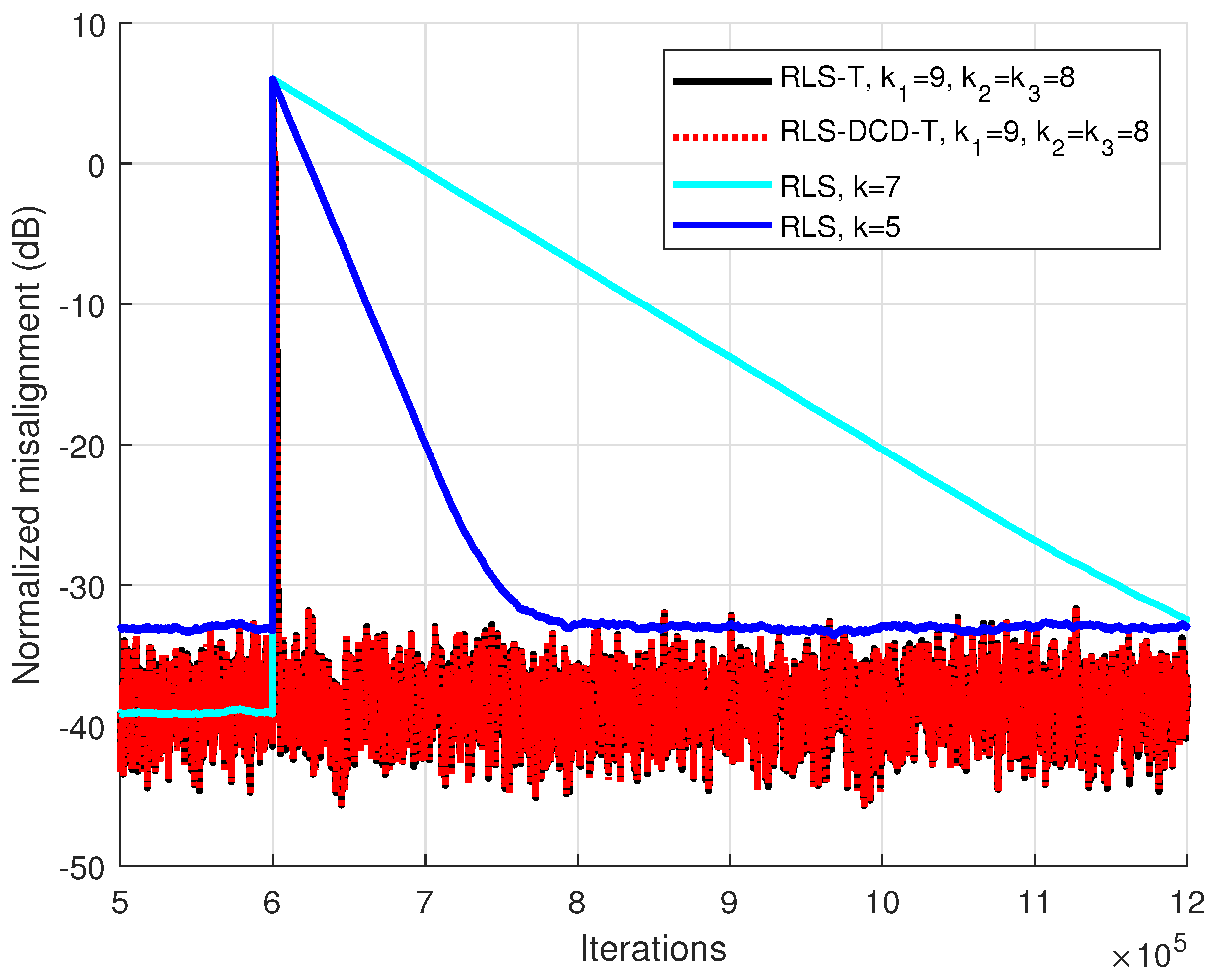
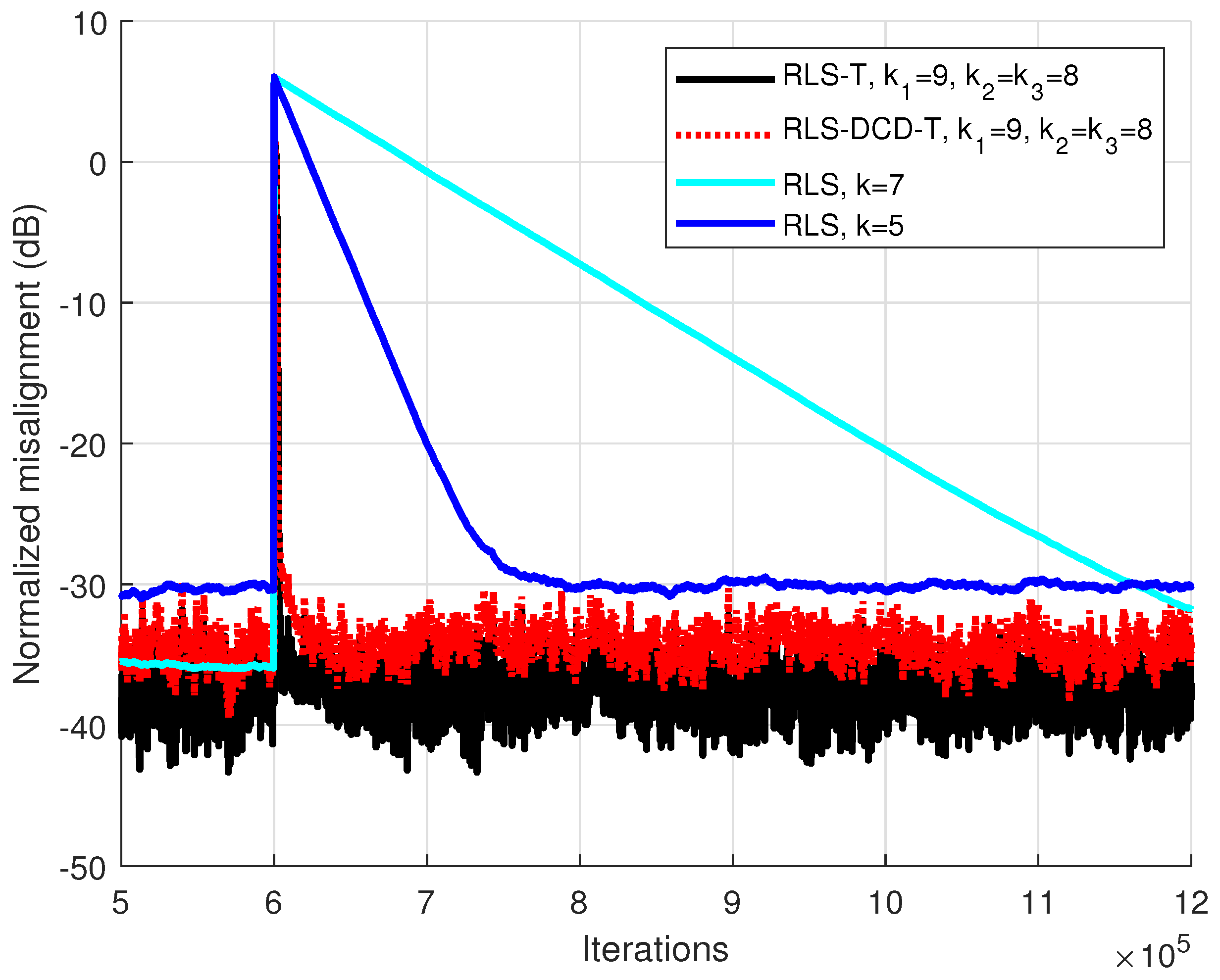
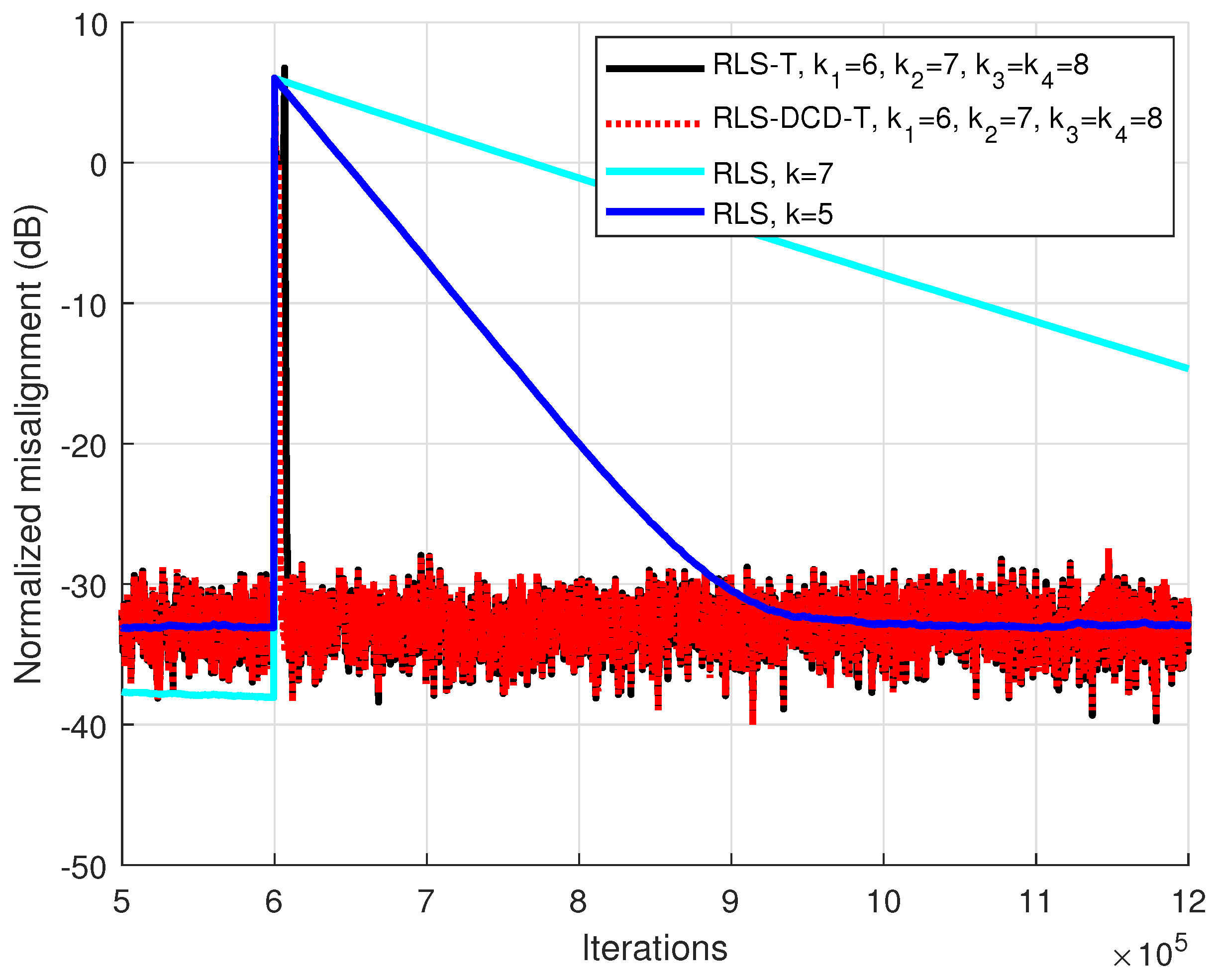
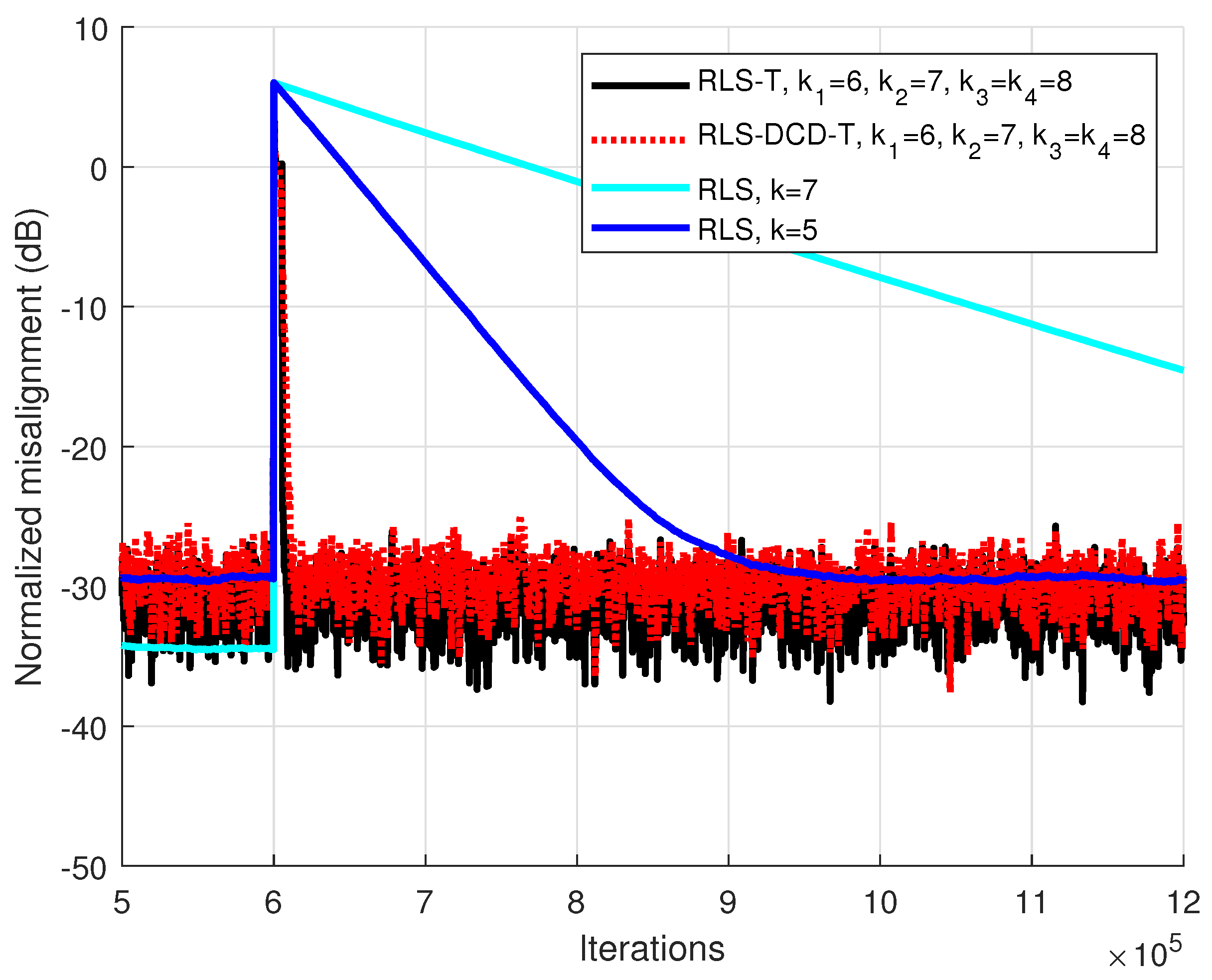
4. Simulations and Practical Considerations

Several sets of experiments were performed in the context of the system identification problem with the MISO configuration. The input signals are white Gaussian noises with sub-unitary values. For some scenarios, before being fed to the input of the system, the signals are also filtered through an auto-regressive AR(1) system with the pole 0.85, in order to create highly-correlated input sequences [11]. For d ( n ) , the signal-to-noise (SNR) ratio is experimentally set to 15 dB.
In the context of adaptive filtering, the convergence behavior and performance analysis of any adaptive algorithm consider the Gaussian input as a benchmark. When the input is white Gaussian noise, the conditional number of the correlation matrix of the input signal is equal to one, since this matrix is a diagonal one and all its eigenvalues are equal. On the other hand, in case of more correlated inputs, the conditional number of this matrix increases, resulting in the challenges in terms of convergence rate. However, the recursive least-squares (RLS) algorithm is less influenced by the character of the input signal (in terms of the correlation degree), as compared to the family of least-mean-square (LMS) algorithms [14]. Consequently, it is important to show that the proposed RLS-DCD-T algorithm also inherits this feature. This is the reason for including both cases in our experiments, i.e., white Gaussian noise and AR(1) process as inputs.
The criterion employed to analyze the performance is the normalized misalignment, corresponding to the global system identification process. It is defined for each time index, using the global filter estimate g ^ ( n ) and the true impulse response g , as 20 log 10 g g ^ ( n ) 2 / g 2 , where · 2 denotes the 2 norm and g is computed based on (8).
The experiments use global impulse responses which can be decomposed using (8) into N = 3 , respectively N = 4 , smaller systems of lengths L i , i = 1 , 2 , , N (depending on the case). The first and the fourth small impulse responses are taken as the first L 1 , respectively L 4 , samples of the the B4 and B1 impulse responses from the G.168 ITU-T Recommendation [28]. The second and third systems are generated using ( 0 . 5 j 1 ) / 2 , respectively ( 0 . 8 j 2 ) / 2 , where j 1 = 0 . . . L 2 1 and j 2 = 0 . . . L 3 1 . In order to evaluate the tracking capabilities of the presented algorithms, the global system is suddenly modified after the initial convergence is achieved by changing the sign of the coefficients corresponding to one of the unknown channels (the longest one, when the case).
The experimental results will mainly compare the performances of the RLS-DCD-T, respectively the RLS-T, adaptive algorithms. For both tensor-based methods, the adaptive filter lengths are chosen as L i = 2 q i and the forgetting factors are set as λ i = 1 1 / ( 2 k i L i ) = 1 1 / ( 2 k i + q i ) . From a hardware implementation point of view, the multiplications with lambda can be performed more efficiently with only bit-shifts and subtractions [18,29]. Furthermore, for the RLS-DCD-T, its DCD specific parameters are chosen considering several aspects. Firstly, the tap values for the estimated systems are sub-unitary ( H = 1 ), and they are represented using M b = 16 bits—one for the sign and the rest, up to 16, hold the magnitude information. Secondly, the maximum number of allowed updates was successfully used in the past with values lower than 10 for adaptive filters with hundreds and thousands of coefficients [18,27]. Taking into account that the selected scenarios have filters with the corresponding lengths L i of maximum tens of coefficients, we chose not to display simulations with N u , i > 1 because they showed no improvement in performance, even for the longer adaptive filters in the tensorial decompositions. For each of the tensor-based update processes (i.e., for each simulated channel), this setting leads to arithmetic complexities proportional to L i .
Although the tensor-based adaptive filters are initialized using the method recommended in [11], the initial convergence is not shown, as it is not considered relevant. For comparison reasons, the classical RLS method based on Woodburry’s identity for the direct identification of the unknown global impulse response is also simulated as a reference, as it is an already validated/established solution in scientific literature. The corresponding forgetting factors were chosen in a similar manner as the equivalent parameters of the tensor based methods (i.e., λ = 1 1 / ( 2 k L ) ).
The first experiments were performed with a configuration of N = 3 filters for the identification of a global system with the length L = 1024 ( L 1 = 64 , L 2 = L 3 = 4 ), where the input signal is Gaussian noise. It can be noticed in Figure 1 that the RLS-DCD-T with N u , i = 1 is enough to generate practically identical performances in comparison to the RLS-T algorithm. Moreover, the RLS adaptive method with different forgetting factors was simulated. It is obvious from the illustration that decreasing the forgetting factor for the RLS in order to increase the tracking speed deteriorates the system identification performance at a convergence state. It is also noteworthy that the individual adaptive filters are connected, i.e., the solution of one filter at time index n depends on the estimates of the other N 1 filters at time index n 1 , due to Equation (19). Consequently, the estimation errors also cumulate in this manner, which could explain the steady-state variation of the tensor-based algorithms (RLS-T and RLS-DCD-T), as compared to the conventional RLS algorithm.
The experiment was repeated for an AR(1) process in Figure 2. Despite the fact that the RLS-DCD-T slightly loses performance in comparison to the RLS-T, similar conclusions can be applied when performing the comparison with the RLS. The tensor based methods outperform the RLS adaptive filter, which cannot simultaneously match them in terms of tracking speed, respectively performance when convergence is achieved.
For the third and fourth scenarios, the MISO configuration was changed to a decomposition based on N = 4 filters. The global system has L = 2048 coefficients and for the tensor-based systems L 1 = 16 , L 2 = 8 , respectively L 3 = L 4 = 4 . In Figure 3, the input signal is Gaussian noise. The performances corresponding to the tensor based algorithms are again very similar. In comparison to the approach which directly identifies the global impulse response (i.e., the RLS algorithm), the RLS-DCD-T and RLS-T have much better tracking capabilities, when targeting for all the methods similar performance after convergence is reached. When repeating the experiment for an AR(1) sequence (Figure 4), it can be considered clear that, for both situations, any attempt of improving the tracking capabilities of the RLS adaptive filter by reducing its memory (i.e., by using a smaller value of λ ) leads to a compromise with the quality the unknown global system identification at the convergence state.
The final scenario analyzes the robustness of the RLS-DCD-T adaptive algorithm in low SNR conditions. The employed MISO configuration is for a global impulse response with L = 4096 , where the tensor based decomposition is performed for N = 4 channels with L 1 = L 2 = L 3 = L 4 = 8 . For an interval of 5000 iterations, the SNR changes from the value of 15 dB to −15 dB. The performances corresponding to the RLS-DCD-T, respectively the RLS-T, are illustrated in Figure 5. The RLS-DCD-T demonstrates the same robustness as the RLS-T when affected by low SNR conditions, with a similar number of iterations required to update its filter coefficients and to achieve again the previous misalignment for the global system estimate g ^ ( n ) .

5. Conclusions

This paper proposed a low-complexity adaptive algorithm for the identification of unknown systems based on tensorial decompositions. We used as a starting point the RLS-T adaptive method, and we developed a new algorithm based on the combination between the exponentially weighted RLS and the DCD iterations. The newly RLS-DCD-T method benefits from the low computational requirements of the DCD and provides performance comparable with other established versions of tensorial based RLS methods. The reduction in complexity for the adaptive filter update process is twofold. Firstly, the RLS-DCD-T benefits from the tensorial approach and solves multiple smaller system identification problems instead of a single problem, which is prohibitive for practical applications. Secondly, the usage of the DCD iterations allows for the coefficient updates to be performed using only bit-shifts and additions.
In future works, we aim to further develop the combination between the least-squares methods and the DCD working within the tensorial decomposition framework. The DCD will be paired with sliding windows versions of the RLS. Moreover, we will develop various methods for increasing the robustness of the RLS-DCD-T in very low SNR conditions, with minimal additions to the arithmetic complexity.

Author Contributions

Conceptualization, C.-L.S., C.E.-I.; Formal analysis, C.A.; Methodology, C.-L.S., C.E.-I.; Software, I.-D.F., C.-L.S. All authors have read and agreed to the published version of the manuscript.

Funding

This work was supported by a grant of the Romanian Ministry of Education and Research, CNCS–UEFISCDI, project number PN-III-P1-1.1-TE-2019-0529, within PNCDI III.

Institutional Review Board Statement

Not applicable.

Informed Consent Statement

Not applicable.

Data Availability Statement

The data presented in this study are available on request from the corresponding author.

Conflicts of Interest

The authors declare no conflict of interest.

References

  1. Andrzej, C.; Rafal, Z.; Anh, H.P.; Shun-ichi, A. Nonnegative Matrix and Tensor Factorizations: Applications to Exploratory Multi-Way Data Analysis and Blind Source Separation; John Wiley and Sons, Ltd.: Hoboken, NJ, USA, 2009. [Google Scholar]
  2. Boussé, M.; Debals, O.; De Lathauwer, L. A Tensor-Based Method for Large-Scale Blind Source Separation Using Segmentation. IEEE Trans. Signal Process. 2017, 65, 346–358. [Google Scholar] [CrossRef]
  3. Ribeiro, L.N.; de Almeida, A.L.F.; Mota, J.C.M. Separable linearly constrained minimum variance beamformers. Signal Process. 2019, 158, 15–25. [Google Scholar] [CrossRef]
  4. Cichocki, A.; Mandic, D.; De Lathauwer, L.; Zhou, G.; Zhao, Q.; Caiafa, C.; Phan, H.A. Tensor Decompositions for Signal Processing Applications: From two-way to multiway component analysis. IEEE Signal Process. Mag. 2015, 32, 145–163. [Google Scholar] [CrossRef] [Green Version]
  5. Sidiropoulos, N.D.; De Lathauwer, L.; Fu, X.; Huang, K.; Papalexakis, E.E.; Faloutsos, C. Tensor Decomposition for Signal Processing and Machine Learning. IEEE Trans. Signal Process. 2017, 65, 3551–3582. [Google Scholar] [CrossRef]
  6. Da Costa, M.N.; Favier, G.; Romano, J.M.T. Tensor modelling of MIMO communication systems with performance analysis and Kronecker receivers. Signal Process. 2018, 145, 304–316. [Google Scholar] [CrossRef] [Green Version]
  7. Rugh, W. Nonlinear System Theory: The Volterra/Wiener Approach. 1981. Available online: https://www.jstor.org/stable/2029400 (accessed on 14 September 2021).
  8. Dogariu, L.M.; Ciochină, S.; Paleologu, C.; Benesty, J.; Oprea, C. An Iterative Wiener Filter for the Identification of Multilinear Forms. In Proceedings of the 2020 43rd International Conference on Telecommunications and Signal Processing (TSP), Milan, Italy, 7–9 July 2020; pp. 193–197. [Google Scholar] [CrossRef]
  9. Dogariu, L.M.; Ciochină, S.; Benesty, J.; Paleologu, C. An Iterative Wiener Filter for the Identification of Trilinear Forms. In Proceedings of the 2019 42nd International Conference on Telecommunications and Signal Processing (TSP), Budapest, Hungary, 1–3 July 2019; pp. 88–93. [Google Scholar] [CrossRef]
  10. Fîciu, I.D.; Stanciu, C.; Anghel, C.; Paleologu, C.; Stanciu, L. Combinations of Adaptive Filters within the Multilinear Forms. In Proceedings of the 2021 International Symposium on Signals, Circuits and Systems (ISSCS), Iasi, Romania, 15–16 July 2021; pp. 1–4. [Google Scholar] [CrossRef]
  11. Dogariu, L.M.; Stanciu, C.L.; Elisei-Iliescu, C.; Paleologu, C.; Benesty, J.; Ciochină, S. Tensor-Based Adaptive Filtering Algorithms. Symmetry 2021, 13, 481. [Google Scholar] [CrossRef]
  12. Dogariu, L.M.; Paleologu, C.; Benesty, J.; Oprea, C.; Ciochină, S. LMS Algorithms for Multilinear Forms. In Proceedings of the 2020 International Symposium on Electronics and Telecommunications (ISETC), Timisoara, Romania, 5–6 November 2020; pp. 1–4. [Google Scholar] [CrossRef]
  13. Dogariu, L.M.; Ciochină, S.; Benesty, J.; Paleologu, C. System Identification Based on Tensor Decompositions: A Trilinear Approach. Symmetry 2019, 11, 556. [Google Scholar] [CrossRef] [Green Version]
  14. Haykin, S. Adaptive Filter Theory, 4th ed.; Prentice Hall: Upper Saddle River, NJ, USA, 2002. [Google Scholar]
  15. Elisei-Iliescu, C.; Paleologu, C.; Benesty, J.; Stanciu, C.; Anghel, C.; Ciochină, S. A Multichannel Recursive Least-Squares Algorithm Based on a Kronecker Product Decomposition. In Proceedings of the 2020 43rd International Conference on Telecommunications and Signal Processing (TSP), Milan, Italy, 7–9 July 2020; pp. 14–18. [Google Scholar] [CrossRef]
  16. Cioffi, J.; Kailath, T. Fast, recursive-least-squares transversal filters for adaptive filtering. IEEE Trans. Acoust. Speech Signal Process. 1984, 32, 304–337. [Google Scholar] [CrossRef]
  17. Stanciu, C.; Ciochină, S. A robust dual-path DCD-RLS algorithm for stereophonic acoustic echo cancellation. In Proceedings of the International Symposium on Signals, Circuits and Systems ISSCS2013, Iasi, Romania, 11–12 July 2013; pp. 1–4. [Google Scholar] [CrossRef]
  18. Stanciu, C.; Anghel, C. Numerical properties of the DCD-RLS algorithm for stereo acoustic echo cancellation. In Proceedings of the 2014 10th International Conference on Communications (COMM), Bucharest, Romania, 29–31 May 2014; pp. 1–4. [Google Scholar] [CrossRef]
  19. Liu, J.; Zakharov, Y.V.; Weaver, B. Architecture and FPGA Design of Dichotomous Coordinate Descent Algorithms. IEEE Trans. Circuits Syst. Regul. Pap. 2009, 56, 2425–2438. [Google Scholar] [CrossRef]
  20. Zakharov, Y.V.; White, G.P.; Liu, J. Low-Complexity RLS Algorithms Using Dichotomous Coordinate Descent Iterations. IEEE Trans. Signal Process. 2008, 56, 3150–3161. [Google Scholar] [CrossRef] [Green Version]
  21. Stenger, A.; Kellermann, W. Adaptation of a memoryless preprocessor for nonlinear acoustic echo cancelling. Signal Process. 2000, 80, 1747–1760. [Google Scholar] [CrossRef]
  22. Huang, Y.; Skoglund, J.; Luebs, A. Practically efficient nonlinear acoustic echo cancellers using cascaded block RLS and FLMS adaptive filters. In Proceedings of the 2017 IEEE International Conference on Acoustics, Speech and Signal Processing (ICASSP), New Orleans, LA, USA, 5–9 March 2017; pp. 596–600. [Google Scholar] [CrossRef]
  23. Benesty, J.; Cohen, I.; Chen, J. Array Processing–Kronecker Product Beamforming; Springer: Cham, Switzerland, 2019. [Google Scholar]
  24. Benesty, J.; Paleologu, C.; Ciochină, S. On the Identification of Bilinear Forms with the Wiener Filter. IEEE Signal Process. Lett. 2017, 24, 653–657. [Google Scholar] [CrossRef]
  25. Bertsekas, D. Nonlinear Programming; Athena Scientific: Belmont, MA, USA, 1999. [Google Scholar]
  26. Elisei-Iliescu, C.; Dogariu, L.M.; Paleologu, C.; Benesty, J.; Enescu, A.A.; Ciochină, S. A Recursive Least-Squares Algorithm for the Identification of Trilinear Forms. Algorithms 2020, 13, 135. [Google Scholar] [CrossRef]
  27. Stanciu, C.; Benesty, J.; Paleologu, C.; Gänsler, T.; Ciochină, S. A widely linear model for stereophonic acoustic echo cancellation. Signal Process. 2013, 93, 511–516. [Google Scholar] [CrossRef]
  28. Digital Network Echo Cancellers. ITU-T Recommendations G.168. Available online: https://www.itu.int/rec/T-REC-G.168/en (accessed on 21 August 2021).
  29. Stanciu, C.; Anghel, C.; Stanciu, L. Efficient FPGA implementation of the DCD-RLS algorithm for stereo acoustic echo cancellation. In Proceedings of the 2015 International Symposium on Signals, Circuits and Systems (ISSCS), Iasi, Romania, 9–10 July 2015; pp. 1–4. [Google Scholar] [CrossRef]
Figure 1. Performance of the RLS-T, RLS-DCD-T, and RLS algorithms, for the identification of the global impulse response g . The tensor-based filters have q 1 = 6 , and q 2 = q 3 = 2 . The input signal is Gaussian noise, N = 3 , and L = 1024 . Both RLS versions have forgetting factors with the form λ = 1 1 / ( 2 k L ) . The performance of the RLS-T and the RLS-DCD-T are almost identical.
Applsci 11 08656 g001
Figure 2. Performance of the RLS-T, RLS-DCD-T, and RLS algorithms, for the identification of the global impulse response g . The tensor-based filters have q 1 = 6 , and q 2 = q 3 = 2 . The input signal is an AR(1) sequence with the pole 0.85, N = 3 , and L = 1024 . Both RLS versions have forgetting factors with the form λ = 1 1 / ( 2 k L ) .
Applsci 11 08656 g002
Figure 3. Performance of the RLS-T, RLS-DCD-T, and RLS algorithms, for the identification of the global impulse response g . The tensor-based filters have q 1 = 4 , q 2 = 3 , and q 3 = q 4 = 2 . The input signal is a Gaussian noise, N = 4 , and L = 2048 . Both RLS versions have forgetting factors with the form λ = 1 1 / ( 2 k L ) . The performance of the RLS-T and the RLS-DCD-T is almost identical.
Applsci 11 08656 g003
Figure 4. Performance of the RLS-T, RLS-DCD-T, and RLS algorithms, for the identification of the global impulse response g . The tensor-based filters have q 1 = 4 , q 2 = 3 , and q 3 = q 4 = 2 . The input signal is an AR(1) sequence with the pole 0.85, N = 4 , and L = 2048 . Both RLS versions have forgetting factors with the form λ = 1 1 / ( 2 k L ) .
Applsci 11 08656 g004
Figure 5. Performance of the RLS-T and RLS-DCD-T for the identification of the global impulse response g . The tensor-based filters have q 1 = q 2 = q 3 = q 4 = 3 . The input signal is an AR(1) sequence with the pole 0.85, N = 4 , and L = 4096 . Between iterations 90001 and 95000, the SNR is set to −15 dB.
Applsci 11 08656 g005
Publisher’s Note: MDPI stays neutral with regard to jurisdictional claims in published maps and institutional affiliations.

