A Variable Ranking Method for Machine Learning Models with Correlated Features: In-Silico Validation and Application for Diabetes Prediction

Featured Application

The methodology proposed in this paper allows to perform robust variable ranking in statistical learning or machine learning models with highly correlated features.

Abstract

When building a predictive model for predicting a clinical outcome using machine learning techniques, the model developers are often interested in ranking the features according to their predictive ability. A commonly used approach to obtain a robust variable ranking is to apply recursive feature elimination (RFE) on multiple resamplings of the training set and then to aggregate the ranking results using the Borda count method. However, the presence of highly correlated features in the training set can deteriorate the ranking performance. In this work, we propose a variant of the method based on RFE and Borda count that takes into account the correlation between variables during the ranking procedure in order to improve the ranking performance in the presence of highly correlated features. The proposed algorithm is tested on simulated datasets in which the true variable importance is known and compared to the standard RFE-Borda count method. According to the root mean square error between the estimated rank and the true (i.e., simulated) feature importance, the proposed algorithm overcomes the standard RFE-Borda count method. Finally, the proposed algorithm is applied to a case study related to the development of a predictive model of type 2 diabetes onset.

1. Introduction

Machine learning (ML) techniques are increasingly being adopted in a variety of medical applications for the development of clinical predictive models, i.e., models for the prediction of outcomes of clinical interest, using a set of candidate variables or features. When building a clinical predictive model with ML, two common problems are variable ranking and variable selection.

Variable ranking, i.e., the ordering of features based on their importance for outcome prediction [1], is useful both to provide an interpretation of the model, i.e., to compare the predictive ability of different variables, and to perform a feature selection, or model reduction, i.e., to identify the most important features and consequently remove the unnecessary variables from the model. The feature selection is important for several reasons. First, models with a large number of input variables can be more difficult to interpret: noisy features, which are not related to the outcome, can have small and implausible effects in the identified model [2]. Noisy features can also lead to an overfitting of the training set data, with consequent poor generalization ability of the model on new previously unseen datasets. Moreover, the models with many input variables are not easy to implement in the clinical practice because some variables may be difficult to collect in different clinical contexts [3].

A simple and popular approach to perform variable ranking is recursive feature elimination (RFE), an iterative algorithm that starts from the full model, i.e., the model including all the variables, and then removes the variables one at the time, dropping at each iteration the least important one. The order of feature removal determines the variable ranking. Once the ranking is obtained, feature selection can be performed by selecting the set of top ranked variables according to a certain criterion.

RFE was originally proposed to perform gene selection for cancer classification using a support vector machine (SVM) model [4]. Then, the algorithm was used for a multitude of applications. For example, RFE and SVM were recently used for classifying attention deficit/hyperactivity disorder [5], multiple sclerosis relapses [6], the management of patients with chronic obstructive pulmonary disease [7], and for selection of heart variability features for cumulative stress monitoring [8]. RFE was also used in combination with other ML models, such as logistic regression (e.g., for Alzheimer’s disease classification [9]), random forest (e.g., for breast cancer classification [10]), and extreme gradient boosting (e.g., for predicting clinical outcomes in young patients with hypertension [11]). Indeed, an advantage of RFE is that it can be applied with any ML model. However, a difficulty of this approach is that the feature ranking can become unstable and sensitive to small perturbations of the training set, potentially resulting in different selected feature sets [12].

In order to assess the stability of variable ranking and perform a robust variable ranking, resampling techniques (with or without replacement) are commonly applied to the original training set in order to produce B different versions of the training set. Then, RFE is performed on each training set version, producing B ranked lists that are combined in order to obtain a global ranked variable list. The most straightforward way to aggregate the B different ranked lists is to use the Borda count method [13], an algorithm well known in voting theory that assigns a score equal to the sum of the number of features with higher position over the B lists to each variable. Then, the global ranked list is obtained by ordering the features according to the Borda count. The Borda count method is equivalent to ranking the features according to their average rank obtained over the B lists. The RFE- Borda count method has been used in many applications [14,15].

Nevertheless, the RFE-Borda count approach can be affected by the presence of correlated features. Indeed, if two highly correlated and highly predictive features, x₁ and x₂, are present in the set of candidate variables, there is a risk that the rank of the two correlated features, which carry a similar information, is underestimated. In fact, it may happen that, in some of the training set resamplings, x₁ gets a high importance score, while x₂, redundant with respect to x₁, gets a low importance score, and the exact opposite might occur (i.e., the importance score is high for x₂ and low for x₁) on other occasions. In such a situation, the importance score would be underestimated for both x₁ and x₂, even if the two features independently bring an important information.

The difficulty of performing variable ranking by RFE in presence of highly correlated features was pointed out by the study of Darst et al. [16]. The authors tested in silico the variable ranking obtained by random forest and RFE. They empirically observed that, when highly correlated features were present in the dataset, the importance score of important predictors was poorly estimated by the RFE algorithm.

One possible solution to this issue, often adopted in the literature, could be to consider only one representative feature for each group of correlated variables in the candidate list of predictors [17]. If there are no practical reasons on which feature to choose, a possibly objective filtering criterion should be adopted. Commonly, the variable that best explains the outcome in a univariate analysis is selected. However, the variable best performing in the univariate analysis could not be the one best performing in the multivariate analysis. In fact, an a priori choice without considering the joint contribution to outcome prediction of all the candidate predictors can result in a suboptimal feature ranking and thus in suboptimal feature selection and model performance. Moreover, even in the case the chosen feature performs optimally in a multivariate framework, it could poorly generalize in a different dataset.

Another option could be to apply a technique for decorrelating the input features, such as the principal component analysis [18]. However, such techniques are suitable to perform dimensionality reduction, not to perform variable ranking or feature selection, and they provide an output set of new features, each obtained from a combination of the original features, whose interpretation is not straightforward.

A different approach was proposed in Yousef et al. for selecting significant genes in gene expression studies [19]. To deal with highly correlated genes, the authors first identified clusters of highly correlated genes and then applied RFE to rank the identified clusters and select the most important ones for the final model. The classification accuracy of the model obtained with the recursive cluster elimination was higher than that obtained with standard RFE. This suggests that considering the highly correlated features as a group while performing RFE might enhance the variable ranking accuracy.

The aim of this work is to propose a new variable ranking method that is able to deal with the presence of highly correlated features and to preserve their interpretation. To offer more detail, the proposed method is a modified version of the RFE-Borda count method that takes into account the correlation between numerical features while performing the ranking, by grouping highly correlated features, as carried out in [19]. The proposed approach is validated on simulated datasets, in which the true variable ranking is known, and compared to the standard RFE-Borda count method that does not consider the correlation between features. After the in-silico validation, the proposed raking method is applied to a case study with real data concerning the development of a predictive model of type 2 diabetes (T2D) onset. This is a problem widely studied in the literature, because the increasing incidence of T2D, especially in the young population, could be lowered by early lifestyle changes in at-risk individuals [20,21]. For this reason, several predictive models of T2D onset have been developed, whose objective is the identification of subjects at risk of developing T2D in the next 5–10 years [3,22]. In particular, ML models were shown to achieve promising results in the prediction of T2D based on multiple risk factors [23,24,25]. A ranking of these risk factors, according to their predictive ability, is crucial to identify the most important predictors that need to be targeted by prevention plans. In this context, highly correlated features are often considered for T2D model development (e.g., body mass index and waist circumference [26]). As it will be shown later in this paper, taking into account the correlation between these features is very important to obtain a reliable variable ranking.

2. Materials and Methods

2.1. The Proposed Variable Ranking Algorithm

Let us define as x_i, i = 1, …, N_feat the set of N_feat candidate variables, y the outcome of the predictive model and X_train the set of training data of cardinality n_train. The proposed algorithm works in four steps:

• Identify the groups of highly correlated numerical features. This can be achieved by computing the correlation coefficient (e.g., Spearman) between each pair of numerical features and then grouping the features with pairwise correlation higher than a threshold th (e.g., th = 0.70). Let us define as C_j, j = 1, ..., N_corr the resulting groups of highly correlated features. Then, we will call N_uncorr the total number of uncorrelated features, i.e., all the features not included in any group C_j.
• Resampling the training set X_train to generate B different versions of the training data. This can be achieved, for example, by bootstrap resampling, i.e., randomly sampling with replacement n_train elements from the training set, or by subset selection, i.e., by randomly sampling without replacement a fraction of elements of the training set (e.g., 80%).
• Perform RFE on each of the B training set variants. In this step, each group of correlated features is considered as a single variable; any time a variable from the group C_j is removed from the model, all the other variables in the same group C_j are also removed from the model and given the same rank. The obtained ranking has a number of positions equal to the number of uncorrelated features, N_uncorr, plus the number of groups of highly correlated features, N_corr. Indeed, the highly correlated features in group C_j count in the ranking as a single variable. The ranks are assigned as follows: the variable (or group of variables) that is (are) removed first is assigned a rank equal to N_uncorr + N_corr; the variable (or group of variables) that is (are) removed at the second RFE’s step is assigned a rank equal to N_uncorr + N_corr − 1; and so on, until the last variable (or group of variables) remaining in the model is assigned rank 1. The ordered feature list obtained from each of the B training set variants is called L_b, b = 1, …, B.
• Aggregate the B ordered variable lists, L_b, b = 1, …, B, by the Borda method. This can be achieved by: (i) computing for each variable (or group of variables) the average rank across the B lists; and (ii) defining a new global rank by ordering the variables (or group of variables) according to the average rank. In this final global ranking, the most important feature (or group of features) will have the lowest rank, while the less important feature (or group of features) will have the highest rank.

Note that if no group of highly correlated features is identified (N_corr = 0), the proposed algorithm becomes identical to the standard RFE-Borda count method. Like the standard RFE-Borda count method, the proposed algorithm is general and it can be applied to perform variable ranking with any statistical learning or ML base model. The parameters of the proposed ranking algorithm are the type of correlation to be considered (e.g., Pearson or Spearman), the threshold th to identify the highly correlated features, the number B of training set variants, and the method used to create these variants (e.g., subset selection or bootstrap sampling).

2.2. Generation of In-Silico Data for Algorithm Validation

The proposed algorithm is validated on in-silico data and compared to the standard RFE-Borda count method. As a base model, we consider the Cox proportional hazard model, a semi-parametric model proposed by Cox in 1972 [27], to perform multivariate survival analysis, i.e., to model the time of an event of interest based on a set of input variables. In particular, the Cox model describes the relationship between a set of variables describing the subject, x₁, …, x_n, and the hazard function, h(t), which denotes the probability that an individual who is under observation at a time t has an event at that time. The characteristic equation of the Cox model is the following:

$$\mathrm{h}\left(\mathrm{t}\right){=\mathrm{h}}_0{\left(\mathrm{t}\right)\mathrm{e}}^{{\mathsf{\beta }}_1{\mathrm{x}}_1+\cdots {+\mathsf{\beta }}_{\mathrm{n}}{\mathrm{x}}_{\mathrm{n}}}$$

(1)

where β₁, …, β_n are the coefficients related to the input variables x₁, …, x_n, and h₀(t) is the baseline hazard function, i.e., the hazard function for subjects with x_i = 0, i = 1, …, n. The Cox model is called semi-parametric because it does not make any assumption on the shape of the baseline hazard function ${\mathrm{h}}_0\left(\mathrm{t}\right)$. Indeed, Cox demonstrated that it is possible to estimate the values of β₁, …, β_n without knowing ${\mathrm{h}}_0\left(\mathrm{t}\right)$ by maximizing the partial log-likelihood. For more details about the Cox model, we refer the reader to [28].

Note that we could have chosen a regression or a classification model, such as multiple linear regression or logistic regression, to run the in-silico experiment, but we preferred to use a survival model because survival analysis is the most natural approach to address the problem presented in the case study of Section 2.3. In the subsections below, we describe in detail how the in-silico data were generated.

2.2.1. Method for Generating Simulated Datasets

In this simulation, we assume that the training set, on which the model is built, includes the observations of n_train subjects, each described by N_feat variables, or candidate predictors. In addition, we assume that the N_feat candidate predictors are normally distributed and that the true model to be identified is a Cox model including a subset of the candidate predictors consisting of the first N_pred variables. The equation of the model is then:

$$\mathrm{h}\left(\mathrm{t}\right){=\mathrm{h}}_0{\left(\mathrm{t}\right)\mathrm{e}}^{{\mathsf{\beta }}_1{\mathrm{x}}_1+\cdots {+\mathsf{\beta }}_{{\mathrm{N}}_{\mathrm{pred}}}{\mathrm{x}}_{{\mathrm{N}}_{\mathrm{pred}}}}$$

(2)

where x₁,…,x_Npred are the true predictors and β₁, …, β_Npred are the related coefficients. The absolute value of the coefficients, |β_i|, defines the predictors’ importance. For simplicity, we assume that |β₁|> … >|β_Npred|, i.e., x₁, is the most important predictor and x_Npred is the least important one.

Of the remaining N_feat − N_pred variables, we assume that N_corr variables, i.e., ${\mathrm{x}}_{{\mathrm{N}}_{\mathrm{pred}}+1},\cdots$, ${\mathrm{x}}_{{\mathrm{N}}_{\mathrm{pred}}{+\mathrm{N}}_{\mathrm{corr}}}$, present a high correlation with some of the N_pred variables that contribute to the true model. In particular, for sake of simplicity, we assume that each group of correlated features in the simulated dataset is made of only two variables, one from the N_pred variables that define the outcome, the other from the N_corr variables that are correlated with the variables that define the outcome, but do not directly contribute to the computation of the outcome. The remaining N_noise = N_feat − N_pred − N_corr variables are noise variables, completely uncorrelated from all the other features.

The N_feat candidate predictors of the training set are generated by extracting n_train random samples from a multivariate Gaussian distribution with dimension N_feat and mean vector M and covariance matrix S. S is diagonal and symmetric, with only N_corr values greater than 0 under and above the diagonal, corresponding to the pairs of correlated features.

The outcome of the model is defined by a vector of event/censoring times, T, and a paired vector of death/censoring indicators, D, both with n_train samples. We initially suppose to know the event time for all the n_train virtual subjects. The event times are generated by multiplying the subjects’ true risk scores, i.e., ${\mathsf{\beta }}_1{\mathrm{x}}_1+\cdots {+\mathsf{\beta }}_{{\mathrm{N}}_{\mathrm{pred}}}{\mathrm{x}}_{{\mathrm{N}}_{\mathrm{pred}}}$, for a suitable scaling factor and finally adding a random normally-distributed noise, with mean equal to 0 and coefficient of variation CV. All the event times are greater than 0, which represents the start of the hypothetical observation period. Then, a certain fraction, F_c, of the virtual subjects is censored; we randomly select F_c*n_train virtual subjects, set their censoring/death indicator to 0, and assign a censoring time chosen at random between 0 and their hypothetical event time to them. For all the non-censored subjects, the event time is supposed to be known, so their value of T is set to the event time and their death/censoring indicator is set to 1.

The relevant parameters of the data simulation algorithm are: N_feat, N_pred, N_corr, N_noise, n_train, CV, F_c.

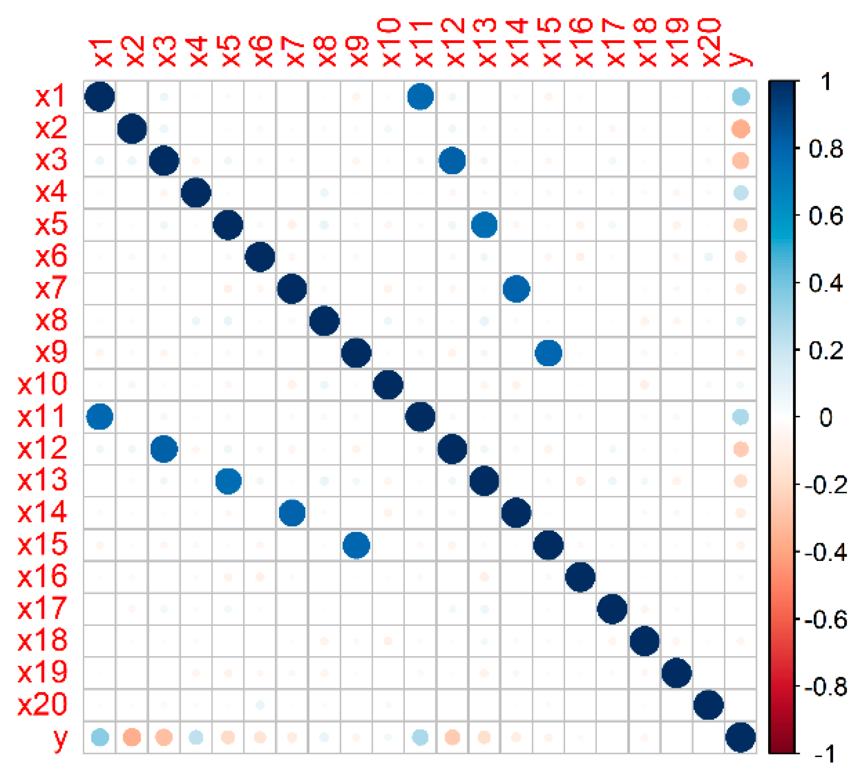
2.2.2. Generation of a Representative Simulated Dataset

A representative simulated dataset was generated with N_feat = 20, N_pred = 10, N_corr = 5, N_noise = 5, n_train = 1000, CV = 30%, and F_c = 0.1. The true model coefficients β₁-β₁₀, corresponding to the true predictors x₁-x₁₀, are reported in

Table 1. Coefficients of the true Cox model for the representative simulated dataset.

Variable	Model Coefficient
x1	4.77
x2	−4.69
x3	−3.74
x4	2.93
x5	−2.74
x6	−2.29
x7	−1.52
x8	1.02
x9	−0.88
x10	0.70

. Note that the features x₁–x₁₀ are ordered by their importance (i.e., by the absolute value of the coefficient in the true Cox model). The features x₁₁, x₁₂, x₁₃, x₁₄, x₁₅ were generated in a way to be highly correlated with variables x₁, x₃, x₅, x₇, x₉, respectively. Finally, the features x₁₆–x₂₀ are uncorrelated from all the other features. The Pearson correlation matrix for this representative simulated dataset is shown in Figure 1.

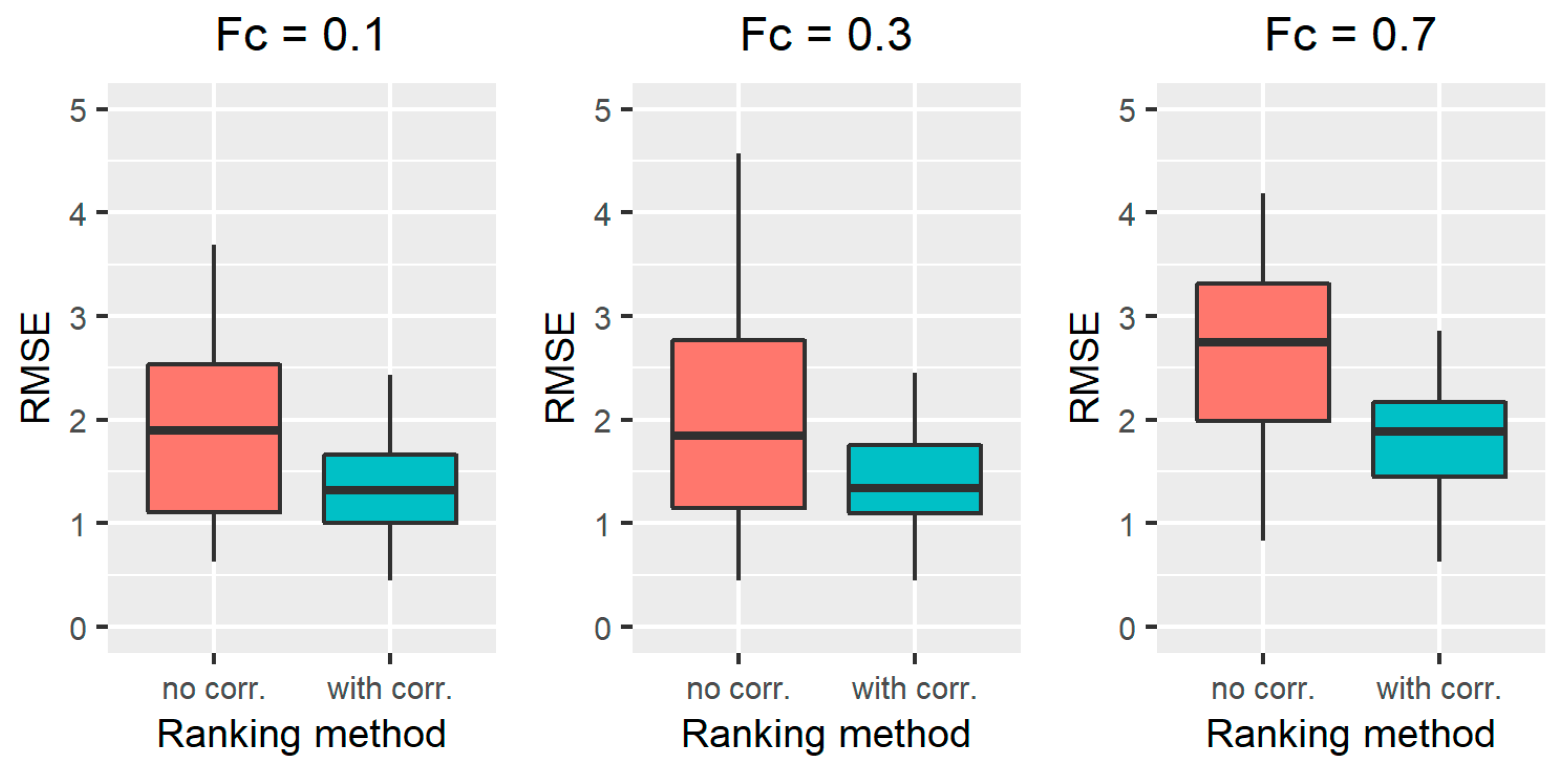
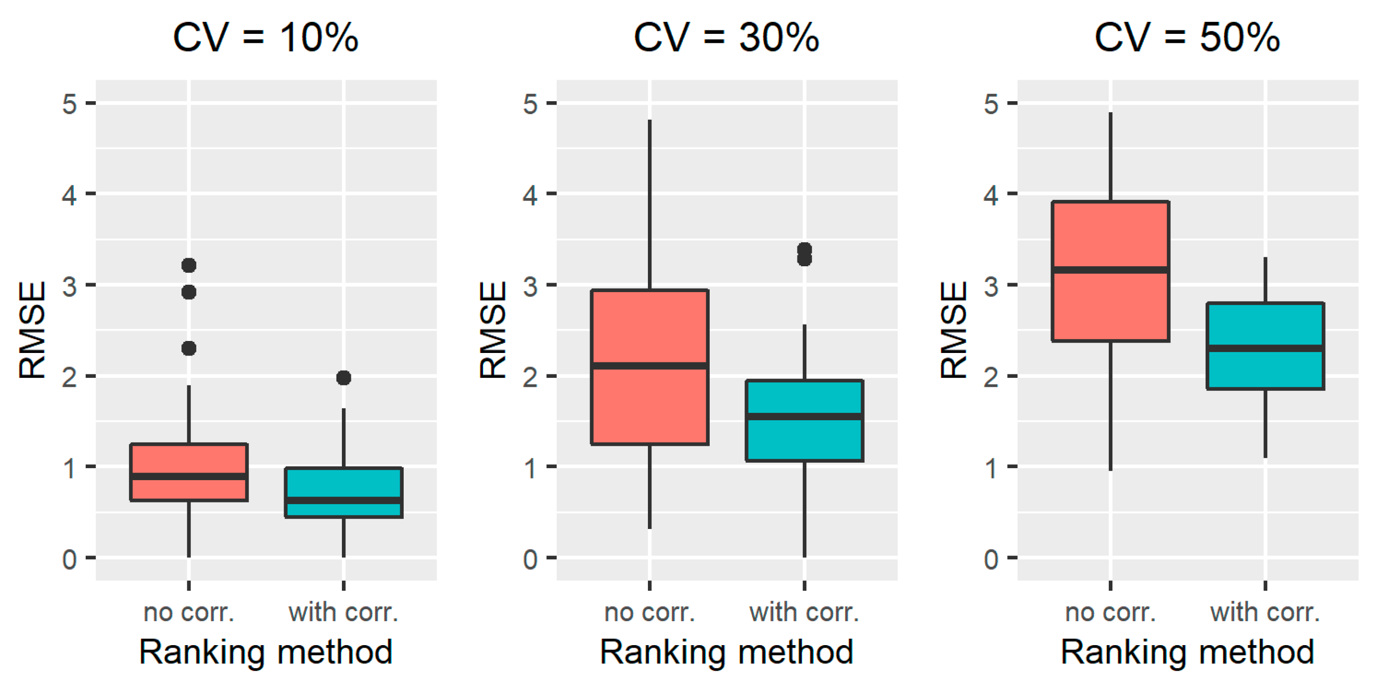
2.2.3. Generation of Different Simulated Scenarios

The parameters of the simulation algorithm were varied in order to test the ranking algorithm in different data scenarios. In total, 12 different simulation scenarios were considered, which are summarized in

Table 2. Summary of simulated scenarios.

Scenario	CV	Nnoise	ntrain	Fc	Npred	Ncorr	Nfeat
1	10%	5	1000	0.5	10	5	20
2	30%	5	1000	0.5	10	5	20
3	50%	5	1000	0.5	10	5	20
4	30%	3	1000	0.5	11	6	20
5	30%	9	1000	0.5	7	4	20
6	30%	12	1000	0.5	5	3	20
7	30%	5	250	0.5	10	5	20
8	30%	5	500	0.5	10	5	20
9	30%	5	1500	0.5	10	5	20
10	30%	5	1000	0.1	10	5	20
11	30%	5	1000	0.3	10	5	20
12	30%	5	1000	0.7	10	5	20

. The first 3 scenarios are characterized by different CV values, for which we tested 3 values: 10%, 30%, and 50%. Scenarios 4–6 are obtained by testing different values for N_noise, i.e., 3, 9, 12, which correspond to the values 11, 7, 5 for N_pred and 6, 4, 3 for N_corr. In scenarios 7–9, we test different values of n_train, i.e., 250, 500, and 1500. Finally, the last 3 scenarios are characterized by different fractions of censored subjects, i.e., 0.1, 0.3 and 0.7. For each scenario, N = 50 training sets were simulated for a total of 600 simulated datasets.

2.3. A Case Study with Real Data: Prediction of Type 2 Diabetes Onset

Besides the assessment with simulated data, the proposed algorithm was tested on a case study with real data, focused on the prediction of T2D onset.

T2D commonly appears in people over 45 because of a combination of genetic and lifestyle factors. The major risk factor for T2D onset is obesity [29]. An early prediction of T2D onset is important because early interventions on modifiable risk factors can post-pone or even prevent the incidence of the disease [20,21]. Predictive models of T2D onset can help in identifying the high-risk subjects who may benefit from targeted prevention measures. Many literature studies focused on the development of a predictive model of T2D onset [3,22]. Some of them also performed variable ranking in order to identify the most important predictors of T2D onset and perform feature selection [30]. The Cox model is one of the most popular techniques for building predictive models of T2D onset, as well as the onset of other chronic diseases [30,31,32].

The aim of this case study is to use the Cox model combined with the variable ranking approach presented in Section 2.1 for ranking risk factors of T2D onset and building a predictive model of T2D onset that takes into account the most important factors. The study is conducted using the data collected in the English Longitudinal Study of Ageing (ELSA).

2.3.1. Dataset: The English Longitudinal Study of Ageing

The English Longitudinal Study of Ageing (ELSA) is an ongoing study of health, social wellbeing, and economic circumstances in the English population aged 50 and older, funded by the U.S. National Institute of Ageing and a consortium of UK Government departments [33]. The ELSA sample mostly includes whites (about 98% of the sample). Participants have a face-to-face interview every 2 years and a clinical examination every 4 years. Currently, the study includes 9 waves of data collection covering a period of 17 years (2002–2019). At waves 3, 4, 6, 7, and 9, new participants entered the study to maintain the size of the sample.

2.3.2. Data Pre-Processing

Since the clinical examinations were performed only in even waves, we assigned to each subject a baseline wave among waves 2, 4, and 6 (not wave 8 because the follow-up would have been too short). Specifically, subjects that entered the study in wave 1 were assigned baseline wave 2, subjects that entered in waves 3/4 were assigned baseline wave 4, and subjects recruited in waves 5/6 were assigned baseline wave 6.

We then selected the subjects who (i) were free of diabetes at the baseline wave; (ii) had the clinical examination at the baseline wave; and (iii) had information on diabetes diagnosis in the follow-up period. A subject was defined as having diabetes at baseline if they answered “Yes” to question Q1:“Has a doctor ever told you that you have diabetes or high blood sugar?” or they presented a value of fasting plasma glucose concentration ≥ 126 mg/dL or a value of glycated haemoglobin ≥ 6.5%. Diabetes onset during follow-up was defined as a positive answer to Q1. The time of diabetes onset was defined as the time passed between the baseline visit and the first follow-up wave at which the subject answered “Yes” to Q1. Note that we did not use fasting plasma glucose or glycated haemoglobin to define the outcome because these variables were not collected at all the ELSA waves.

Potential predictive variables for diabetes development were selected from the set of variables collected at the ELSA baseline visits. In total, 16 variables were selected which are reported in

Table 3. Baseline variables selected as candidate predictors for T2D model development.

Variable Name	Description	Values
sex	Sex	0 = females 1 = males
age	Age	Continuous [years]
mar_stat	Marital status	0 = married, living as married 1 = separated, widowed 2 = never married
depriv	Level of economic deprivation	Integers, range 1–5
smoke	Smoking status	0 = never smoked 1 = past smoker 2 = current smoker
phys_act	Frequency of moderate or vigorous physical activity	0 = hardly ever or never 1 = 1–3 times per month 2 = once/week 3 = >once/week
bmi	Body mass index	Continuous [kg/m2]
waist	Waist circumference	Continuous [cm]
sys_bp	Systolic blood pressure	Continuous [mmHg]
depress	CESD-8 depression score	Integers, range 1–8
life_exp	Life expectation	Integers, range 1–100
phealth	Self-reported poor health	Integers, range 1–5
htn	Ever had hypertension	0 = no, 1 = yes
hchol	Ever had high cholesterol	0 = no, 1 = yes
hdl	HDL cholesterol	Continuous [mg/dL]
tot_chol	Total cholesterol	Continuous [mg/dL]

. In particular, economic deprivation was measured by question Q2: “How often you find you have too little money to spend on what you feel you and your household’s needs are?”, whose possible answers (“never”, “rarely”, “sometimes”, “often”, “most of the time”) were coded with integers between 1 and 5. Depression was measured by a reduced version of the Center for Epidemiologic Studies Depression (CESD) scale that includes 8 items. The derived score is an integer going from 1 to 8, with higher values representing a major presence of depression symptoms. Life expectation was coded as a number between 0 and 100, representing the self-reported probability of living to 75 years if the respondent is under 65 years, to 80 years if the respondent is aged 66 to 69 years, and to 85 years if the respondent is aged 70 to 74 years, etc. Self-reported health status was measured on a 5-level scale ranging between “excellent” and “poor”.

Subjects with missing values in any of the selected variables were removed from the analysis. The final selected sample included 6201 subjects, 449 of whom developed diabetes during the 15-year observation period after the baseline.

2.4. Application of the Ranking Algorithms on In-Silico and Real Data

2.4.1. Assessment of the Ranking Algorithms on In-Silico Data

The ability of the proposed algorithm to perform an accurate variable ranking was assessed on the simulated data described in Section 2.2. On each simulated dataset, the variables were ranked considering two approaches:

• Approach 1: standard RFE-Borda count method without considering the correlation between features;
• Approach 2: the proposed algorithm that considers the correlation between features.

For both the approaches, we considered B = 100 bootstrap resamplings of the training set. For the proposed algorithm, a threshold of 0.7 on the Pearson correlation coefficient was used to identify the groups of highly correlated features.

For both the ranking methods, the accuracy of the ranking is assessed by calculating the root mean square error (RMSE) between the estimated ranking and the true ranking. This metric was chosen because it has a very intuitive interpretation and it quantifies the average number of positions mistaken in the ranking, regardless of the direction of the mistake (overestimation or underestimation) and the relative position in the ranked list.

For the simulated scenarios 1–12, in particular, we assessed the RMSE value for each of the N = 50 training sets and then compared the distribution of RMSE between the two ranking algorithms.

2.4.2. Application of the Ranking Algorithms to Real Data

The data selected from the ELSA dataset, as detailed in Section 2.3.2, were randomly split into a training set, containing 80% of selected subjects, and a test set, containing the remaining 20% of subjects, stratifying by diabetes incidence. The training set was used for model development, while the test set was used for final model assessment. Training set variables were scaled in a range 0–1, subtracting to each variable its minimum value and then dividing it for the difference between its maximum and its minimum value. The same scaling was applied to test set data, using the minimum and maximum values of the features in the training set. Categorical variables with more than two levels (i.e., mar_stat and smoke) were re-coded using dummy variables. Physical activity (phys_act) was considered as a numerical variable.

A Cox model for the prediction of T2D onset was trained on the training set by applying the method based on RFE and Borda count to perform variable ranking and feature selection. Before performing the ranking, we analysed the correlation between features in the training set. This analysis revealed the presence of a pair of highly correlated features: BMI and waist circumference have a Spearman correlation coefficient of 0.78. All the other pairs of features present a Spearman correlation coefficient below 0.40. As the presence of this pair of highly correlated features can affect the variable ranking, we performed the ranking considering the two ranking approaches tested in simulation:

• Approach 1: The correlation between BMI and waist circumference is ignored and the standard RFE-Borda count method is applied;
• Approach 2: The ranking is performed with the proposed algorithm that takes into account the correlation between BMI and waist circumference.

To better understand the impact of highly correlated features on the ranking performance of the standard RFE-Borda count method, we also tested two additional approaches in which one correlated feature is removed a priori.

• Approach 3: Waist circumference is dropped from the analysis and the ranking is performed with the standard RFE-Borda count method, considering only BMI in the set of candidate predictors.
• Approach 4: BMI is dropped from the analysis and the ranking is performed with the standard RFE-Borda count method, considering only waist circumference in the set of candidate predictors.

For all the approaches, the training set was resampled with replacement B = 100 times. At each iteration, the resampled training set was used to train the models with decreasing number of features as per the RFE algorithm, while the subjects of the out-of-bag set (i.e., those of the original training set not present in the resampled training set) were used to assess the performance of the models. The performance was assessed by the concordance index (C-index) [34], which measures the concordance between risk scores and event times (0.5 no concordance at all, 1 perfect concordance). The output of the RFE-Borda count method at the end of the B iterations includes:

• a table with the mean and the standard deviation (SD) of the rank obtained for each feature across the B iterations;
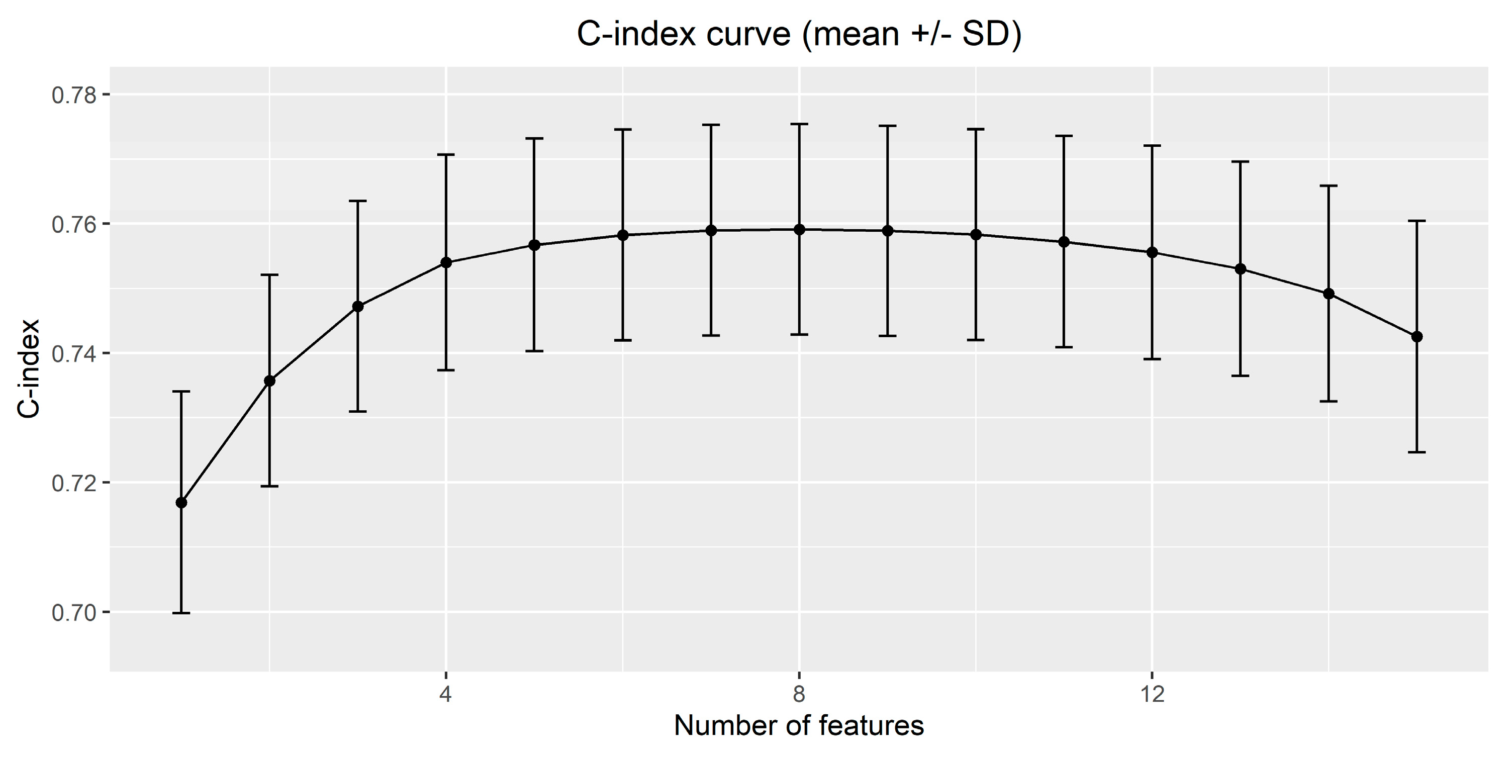
• a table with the value of the C-index (mean and SD) for models with different number of features.

Afterwards, the final feature selection is made by choosing the optimal number of features, n_opt, as the number of features that maximizes the mean of the C-index across the B iterations, and then choosing from the rank table the n_opt variables with highest mean rank. The final step is to train the model with the selected features on the entire training set, and to assess its performance in terms of C-index on the test set. To get a confidence level for the C-index, we also performed a 5-fold cross-validation on the training set and assessed the mean (SD) of C-index on the 5 testing folds.

3. Results

3.1. In-Silico Assessment of the Proposed Variable Ranking Algorithm

3.1.1. Results on a Representative Simulated Dataset

The results of the variable ranking obtained for the representative dataset of Section 2.2.2 are reported in

Table 4. Results of variable ranking for the representative simulated dataset.

Global Rank	Standard RFE-Borda Count Method (without Correlation)		Proposed Algorithm (with Correlation)
	Variable	Mean Rank	Variable	Mean Rank
1	x1	1.29	x1–x11	1.22
2	x3	2.37	x2	2.47
3	x2	2.76	x3–x12	2.47
4	x4	4.55	x4	4.69
5	x6	6.10	x5–x13	5.68
6	x5	6.16	x6	5.94
7	x7	9.53	x7–x14	8.59
8	x15	11.25	x9–x15	10.04
9	x8	11.76	x8	10.15
10	x19	12.73	x10	10.87
11	x18	13.44	x18	11.21
12	x14	13.48	x19	11.28
13	x12	13.61	x20	11.34
14	x9	13.88	x16	11.82
15	x13	13.89	x17	12.23
16	x11	14.08
17	x20	14.38
18	x10	14.47
19	x16	15.01
20	x17	15.26
	RMSE = 3.07		RMSE = 0.50

for both the standard RFE-Borda count method and the proposed algorithm, performed on B = 100 training set variants generated by bootstrap resampling. We can observe that the standard RFE-Borda count approach, which ignores variable correlation, commits some ranking mistakes: x₂ is ranked below x₃; x₅ is ranked in the 6th position, below x₆; x₈ is ranked in the 9th position, after x₁₅; x₉ and x₁₀ are ranked in the 14th and the 18th position, respectively, and they are surpassed in the ranking even by noise variables, such as x₁₈, x₁₉, and x₂₀. Conversely, the ranking obtained by the proposed approach, which considers the variable correlation, is almost completely correct; the only ranking mistake is that, also in this case, x₈ is ranked in the 9th position, after x₉ and its correlated feature x₁₅. We can note that the proposed algorithm always assign the same rank to the highly correlated variables. Overall, the RMSE obtained is 3.07 for the standard RFE-Borda count method and 0.50 for the proposed approach.

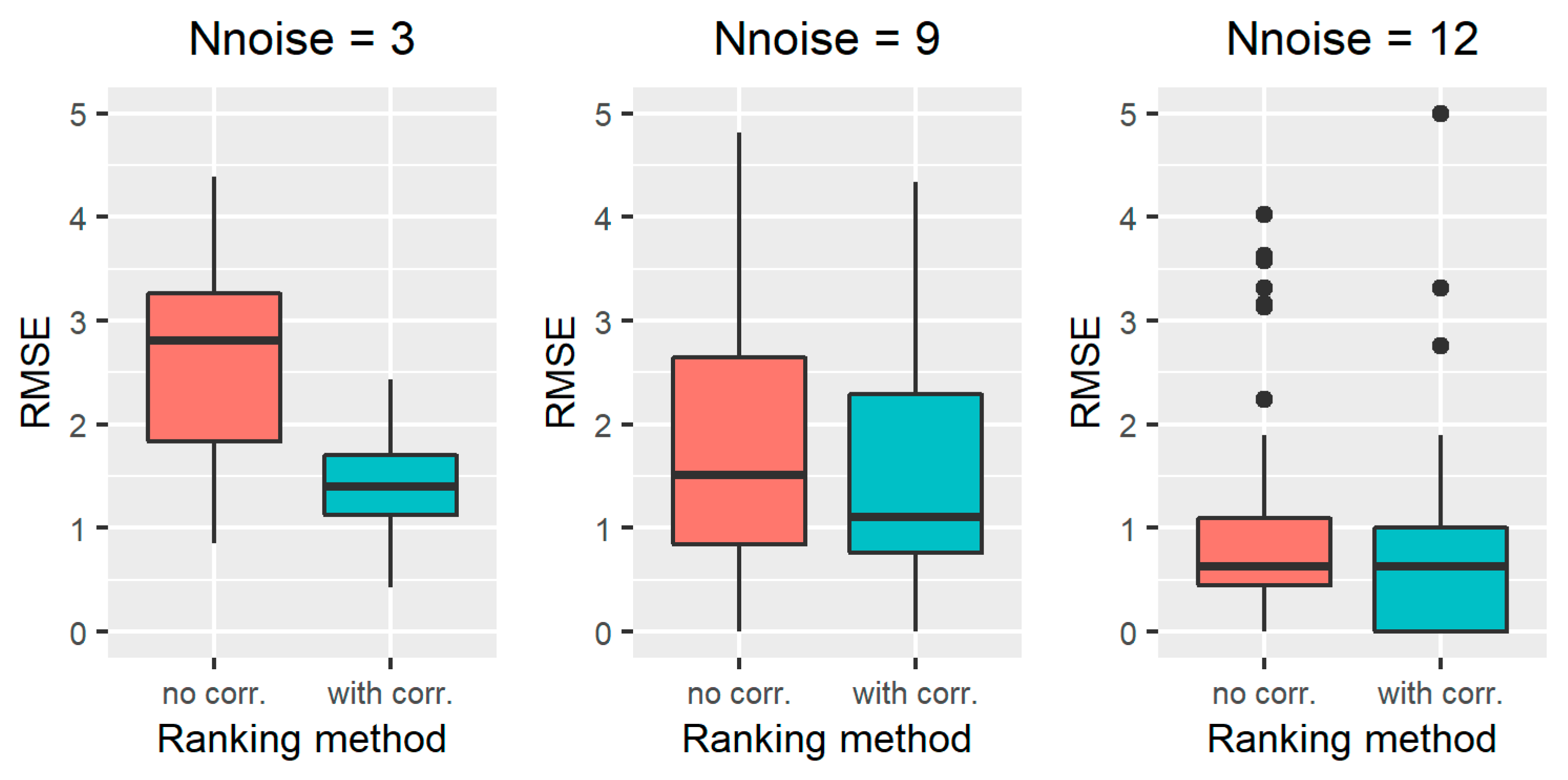
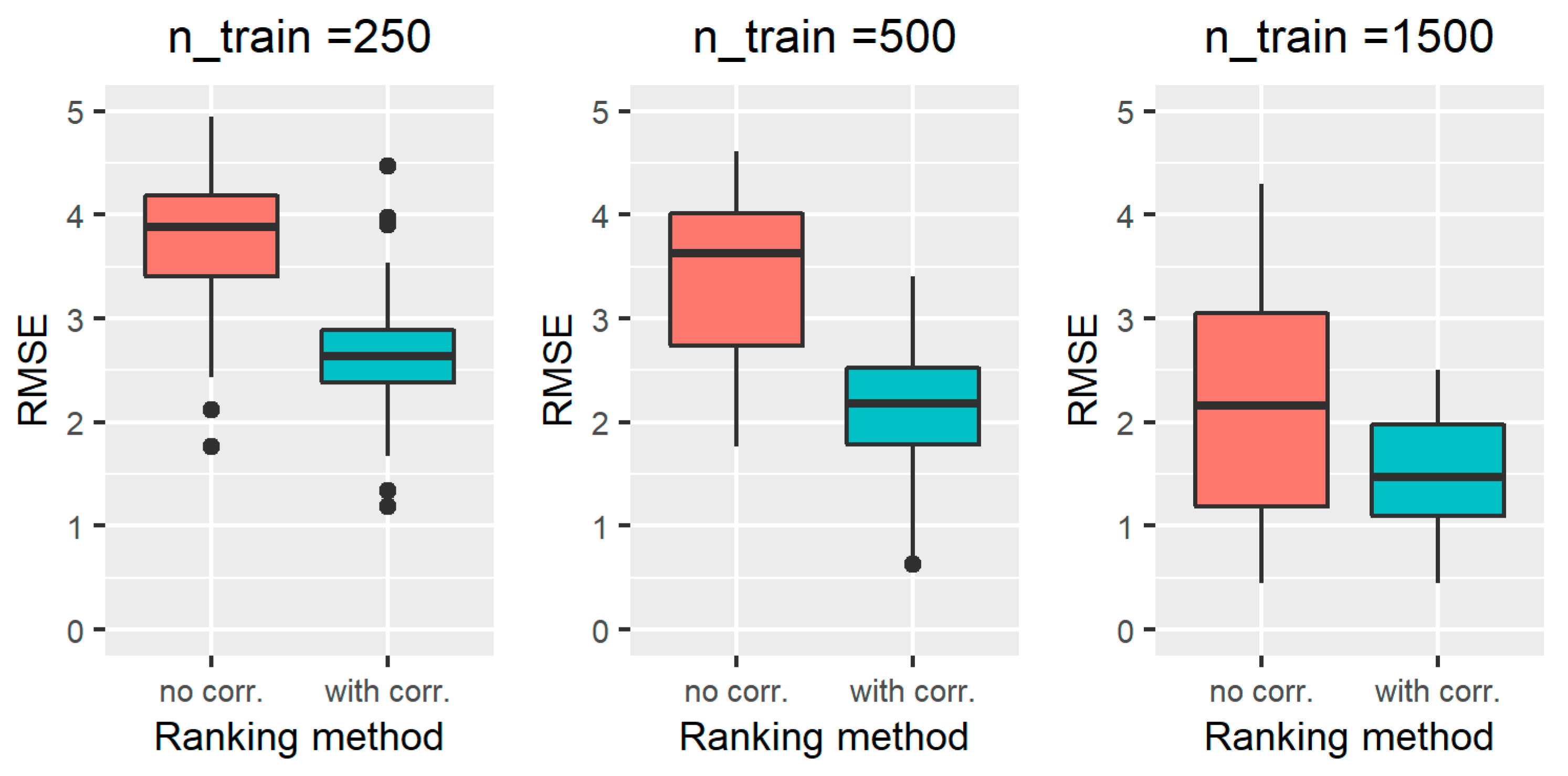
3.1.2. Results on All the Simulated Scenarios

The results obtained on all the simulated scenarios of Section 2.2.3, in terms of ranking performance, are reported in Figure 2 for scenarios 1–3, Figure 3 for scenarios 4-6, Figure 4 for scenarios 7–9, and Figure 5 for scenarios 10–12. In particular, the RMSE distribution obtained for the standard RFE-Borda count method and the proposed algorithm are shown in green and red, respectively. We can observe that, for all the scenarios, the RMSE presents lower values for the proposed approach compared to the standard RFE-Borda count method. The advantage of using the proposed algorithm is very limited for the scenario with very little noise (scenario 1—CV = 10%) and the one with 12 noise variables (scenario 6—N_noise = 12). Indeed, in these scenarios, the standard RFE-Borda count method already performs well with almost 75% of RMSE values below 1. However, for all the other scenarios, the proposed algorithm clearly improves the ranking performance of the standard RFE-Borda count method, as shown by the boxplot of the RMSE that is distributed at lower values for the proposed algorithm.

3.2. Results on the Case Study with Real Data

In this section, we present the results obtained by applying the two variable ranking algorithms, evaluated in-silico in Section 3.1, to the case study about T2D onset prediction, presented in Section 2.3. In this case study, the dataset includes two highly correlated features that represent the concept of obesity: BMI and waist circumference. Since obesity is the leading risk factor for T2D development [29], we expect that the variable ranking algorithms will rank these variables as the top predictors of T2D onset.

The results of variable ranking are shown in

Table 5. Results of variable ranking for the predictive model of T2D onset.

Approach 1		Approach 2		Approach 3		Approach 4
Variable	Mean (SD) of Rank	Variable	Mean (SD) of Rank	Variable	Mean (SD) of Rank	Variable	Mean (SD) of Rank
hdl	2.91 (3.04)	bmi-waist	1.01 (0.10)	bmi	1.02 (0.14)	waist	1.04 (0.24)
sys_bp	3.12 (3.42)	hdl	2.83 (2.78)	hdl	2.74 (3.06)	sys_bp	2.76 (2.79)
bmi	4.47 (4.66)	sys_bp	2.96 (2.98)	sys_bp	2.86 (3.01)	hdl	2.82 (2.48)
waist	4.51 (4.39)	phealth	5.71 (5.00)	phealth	5.44 (4.69)	phealth	5.32 (5.11)
phealth	6.16 (5.42)	depress	6.21 (3.29)	age	6.53 (3.03)	sex	5.48 (3.08)
depress	6.72 (3.41)	age	6.70 (3.19)	depress	6.64 (3.14)	depress	6.65 (3.05)
age	7.23 (3.31)	depriv	7.08 (3.82)	depriv	7.08 (3.72)	htn	7.40 (4.21)
depriv	7.23 (3.31)	htn	7.32 (4.23)	htn	7.59 (4.10)	depriv	7.59 (3.50)
htn	7.95 (4.52)	hchol	8.96 (3.29)	sex	8.32 (3.55)	age	7.98 (2.91)
sex	8.78 (3.74)	tot_chol	8.99 (2.71)	hchol	8.95 (3.10)	hchol	9.22 (2.93)
hchol	9.63 (3.43)	phys_act	9.10 (2.63)	tot_chol	9.13 (2.71)	tot_chol	9.37 (2.62)
tot_chol	9.74 (2.90)	sex	9.27 (2.85)	phys_act	9.42 (2.61)	phys_act	9.52 (2.52)
phys_act	9.85 (2.73)	life_exp	9.52 (2.63)	life_exp	9.58 (2.72)	life_exp	9.82 (2.63)
life_exp	10.17 (2.77)	smoke	10.10 (2.77)	smoke	10.33 (2.69)	mar_stat	10.39 (3.10)
smoke	10.97 (2.79)	mar_stat	10.24 (3.10)	mar_stat	10.37 (2.85)	smoke	10.64 (2.32)
mar_stat	11.06 (3.18)

; for each scenario we report the mean (SD) of the rank obtained for each feature across the B = 100 runs of the RFE algorithm. Lower rank are assigned to the most relevant features. For each scenario, the features were ordered by their mean rank value, which represents the variable importance.

By applying the standard RFE-Borda count algorithm, we can note that, in the approaches 3 and 4, in which only one obesity variable is considered in the set of candidate predictors (the other is a priori excluded), the obesity variables are ranked in the top position of the list, i.e., they are identified as most important predictors. This happens with very high consistency across the 100 iterations, as the average rank is very close to 1 and the SD of the rank is close to 0. However, when BMI and waist circumference are both included in the set of candidate predictors, as in approach 1, and the ranking is performed ignoring the correlation between these features, we can see that the obesity variables are assigned lower importance values. In particular, they are ranked in the third position, after HDL cholesterol and systolic blood pressure, and their rank is much more unstable across the 100 iterations; the SD is around 4, the second-highest value among all the candidate predictors. This means that the estimated rank obtained for these features with the standard RFE-Borda count method is very uncertain. This example confirms what we discussed in the introduction of this paper: the presence of highly correlated features, if not properly managed, can affect the results of variable ranking.

The proposed algorithm is effective in solving this issue. Indeed, looking at the results for approach 2 in Table 5, we can see that the proposed algorithm, which takes into account the correlation between BMI and waist circumference, is able to identify the high predictive ability of the obesity features, which are now ranked again in first position with high confidence (the rank is 1.01 ± 0.1). This result confirms what was already observed in the in-silico study: in presence of highly correlated features, the proposed algorithm allows to perform a more robust variable ranking compared to the standard RFE-Borda count method, without the need of pre-filtering the highly correlated features based on a priori knowledge or assumptions. This aspect is important because an effective pre-filtering of the features, as carried out in approach 3 and 4, could be difficult to perform using just the a priori knowledge, especially when the dataset includes multiple groups of highly correlated features. A bad a priori choice on important predictors could negatively affect the model performance and generalization ability.

After performing the variable ranking, the optimal number of features was selected by analyzing the curves of C-index vs. number of features in the out-of-bag samples. In Figure 6, the C-index curve returned by the proposed algorithm (approach 2) is shown. As expected, the average C-index value increases with the number of features, until a certain plateau is reached. The resulting optimal number of features which maximizes the average C-index value is 8. The same optimal number of features was obtained with approaches 3 and 4, whereas, with approach 1, in which the two obesity variables are treated independently, the optimal number of features is 9.

Table 6. Coefficients and performance of the predictive model of T2D onset obtained in approach 1 (standard RFE-Borda method with both BMI and waist circumference), approach 2 (proposed algorithm, the model with waist is shown), approach 3 (standard RFE-Borda method with BMI only), approach 4 (standard RFE-Borda method with waist circumference only).

Variable	Estimated Coefficient (Standard Error)
	Approach 1	Approach 2	Approach 3	Approach 4
bmi	2.00 (0.62)	-	3.34 (0.38)	-
waist	2.17 (0.75)	4.03 (0.48)	-	4.14 (0.48)
hdl	−1.75 (0.35)	−1.59 (0.34)	−2.11 (0.33)	−1.81 (0.39)
sys_bp	1.69 (0.40)	1.74 (0.40)	1.77 (0.39)	1.81 (0.39)
phealth	0.77 (0.23)	0.82 (0.23)	0.81 (0.23)	0.81 (0.23)
depress	0.22 (1.25)	0.26 (0.23)	0.17 (0.23)	0.20 (0.23)
age	0.40 (0.36)	0.23 (0.35)	0.43 (0.36)	-
depriv	0.38 (0.20)	0.40 (0.20)	0.40 (0.20)	0.36 (0.20)
htn	0.26 (1.30)	0.29 (0.11)	0.26 (0.11)	0.28 (0.11)
sex	-	-	-	−0.21 (0.12)
C-index 5-fold CV	0.75 (0.02)	0.75 (0.03)	0.75 (0.02)	0.75 (0.02)
C-index test	0.74	0.74	0.74	0.75

shows the final models obtained with the four ranking approaches, considering the top 8 variables in Table 5 for approaches 2–4 and the top 9 variables in Table 5 for approach 1. For each approach, we report the estimate (standard error) of the coefficient in the final model trained on the entire training set. Note that, for approach 2, the top predictive variable is the pair of features describing obesity; however, for not introducing redundancy in the model, only one of these two variables was included in the final model. We tested the model with BMI (and the other 7 features) and the model with waist circumference (and the other 7 features) in a 5-fold cross-validation performed on the training set; the model with highest average C-index was the one with waist circumference. The results for this model are then reported in Table 6. We can see that, in all the models, the obesity variables have the highest, in absolute value, coefficient, although, in approach 1, the contribution of obesity is divided between BMI and waist circumference, with resulting lower coefficients for these variables compared to the other approaches. We can also observe that the standard error of obesity variables’ coefficients is higher in approach 1 compared to the other approaches.

Table 6 also reports the discrimination performance of the developed models. All the models achieved similar C-index values, both on the 5-fold cross-validation and on the test set. The C-index values obtained are in line with those of literature models using similar feature sets [3]. Interestingly, in this case study, some variables related to the psychologic and economic wellbeing, not present in most of existing T2D models, were selected by the models. These variables are: the CESD depression scale, the perceived health status, and the self-reported level of economic deprivation.

4. Discussion

As evidenced in a recent simulation study [16], the presence of highly correlated features can negatively affect the performance of the RFE algorithm. A common approach to deal with this issue is to exclude a priori the highly correlated features before the development of the model, by choosing one representative feature for each group of correlated variables. However, an a priori choice without considering the joint contribution to outcome prediction of all the candidate predictors can result in a suboptimal feature ranking and, thus, a suboptimal feature selection and model performance.

To solve the issues that an a priori feature filtering might bring, in this paper we proposed a new ranking algorithm that handles the highly correlated features within the ranking procedure. The algorithm is a modified version of the RFE-Borda count method in which highly correlated features are grouped during the RFE procedure. This ensures that all the features are considered for model development. Then, if a pair of highly correlated features are selected for the final model, e.g., x₁ and x₂, the model developer can decide a posteriori which feature to remove, by comparing the multivariate model with x₁ vs. the multivariate model with x₂, in terms of prediction performance. This would be a better choice than the one made a priori, because it takes into account the presence of all the other variables relevant for the prediction. Moreover, it allows performing variable importance ranking in an unbiased way.

The idea of grouping the correlated features while performing the RFE is not totally new. A similar approach, called recursive cluster elimination, was indeed adopted by Yousef et al. [19] for selecting significant genes in gene expression studies using the SVM model. Youssef et al. showed that the clustering of highly correlated features allowed to improve the final model performance, suggesting that a better feature ranking and feature selection was obtained. However, to the best of our knowledge, the method by Yousef et al. was never validated in terms of variable ranking performance. Moreover, an issue of the method by Youssef et al. is that, after the ranking of clusters and the selection of the most important ones, all the highly correlated features in the selected clusters are included in the final model, thus maintaining a certain level of redundancy in the model.

In this paper, the proposed algorithm was validated on simulated datasets in which the true variable ranking is known. Results showed that the proposed algorithm provides better ranking performance compared to the standard RFE-Borda count method that does not consider the correlation between features. This result was confirmed on 12 different simulation scenarios, in which we varied the noise level on the outcome, the proportion of noise variables in the training set, the number of training set samples, and the fraction of censored data. In all the tested scenarios, the proposed algorithm outperformed the standard RFE-Borda count method, proving its good performance even in challenging scenarios with high noise, small sample sizes, and high censoring fractions.

The proposed algorithm has also been assessed on a real case study, in which the aim was to rank risk factors for T2D onset and to develop a predictive model of T2D onset that takes into account the most important ones. The dataset included more than 6000 subjects, monitored for up to 15 years within a longitudinal study of health conducted in U.K. To test the ranking performance of the proposed algorithm, we included two highly correlated features in the set of candidate predictors (BMI and waist circumference) related to obesity, which is well recognized as the leading risk factor for T2D onset [29]. Nevertheless, the standard RFE-Borda count method failed to estimate with high confidence the rank of these obesity variables, because the high correlation between the two features altered the ranking results. Conversely, the proposed algorithm assigned to the obesity variables the highest importance level, and it was able to estimate their rank with high confidence. This proves what was already verified with simulated data: the proposed algorithm is able to robustly perform variable ranking in the presence of highly correlated features, outperforming the standard RFE-Borda count method.

The developed T2D model included 8 variables: BMI or waist, HDL cholesterol, systolic blood pressure, self-reported poor health level, depression scale, the level of deprivation, history of hypertension, and sex or age. While variables related to obesity, hypertension and hypercholesterolemia are commonly used by literature T2D models [22], a few models considered socio-economic factors, such as deprivation [31] or income [35]. As far as depression is concerned, this variable has never been used in literature T2D models. Nevertheless, several studies found an association between depression symptoms and the incidence of T2D [36]. Our results support this association, as depression was ranked in fifth position by the variable ranking algorithm, immediately after three strong risk factors (i.e., obesity, cholesterol, and hypertension) and the self-reported poor health level.

Regarding the discrimination ability, the developed T2D model achieved comparable performance to that of other literature models assessed on the same dataset [3], e.g., the FINDRISC model [26], the basic model by Kahn et al. [37], and the Atherosclerosis Risk in Communities simple model [38], with a C-index of around 0.75. Other literature models were able to achieve a higher discrimination performance (e.g., C-index > 0.80) by considering among the predictors variables related to dysglycemia, such as fasting plasma glucose, results of the oral glucose tolerance test, and the homeostatic model assessment of insulin resistance and beta cell indices [3,22,30,38].

Although promising results were achieved, the study conducted in this paper presents some limitations that deserve future investigation. A limitation of the proposed algorithm is that it can only deal with highly correlated numerical variables. In future works, the algorithm needs to be extended to deal also with categorical variables. This can be achieved by replacing the correlation coefficient with a suitable measure of the association between categorical variables, such as the Cramer’s V, the phi coefficient, or the mutual information [39].

Other limitations concern the validation procedure. In this paper, the proposed variable ranking algorithm was assessed considering the Cox proportional hazard model as a base model, which was the simplest and most natural approach to address the prediction problem of the presented case study. However, the proposed algorithm is general and can be applied in principle to any ML model. In future works, the proposed algorithm could be tested with different models, including linear and non-linear regression and classification models.

Finally, we recognize that the in-silico assessment performed in this study makes several assumptions. For example, we assumed that the input variables are normally distributed, and that the groups of correlated features are made of only two variables, linearly correlated to each other, of which only one contributes to the outcome. In future works, we will perform a more comprehensive validation of the approach, for example considering variables with different statistical distributions, different types of variable correlation, and different values for the simulation parameters.

5. Conclusions

In this paper, we modified the variable ranking algorithm based on RFE and Borda count to deal with highly correlated numerical features. The proposed algorithm was validated on simulated datasets, showing better ranking performance than the standard RFE-Borda count algorithm. These encouraging results were confirmed on a real case study, conducted on the ELSA dataset, regarding the prediction of the T2D onset. In future works, the algorithm will be extended to deal with categorical variables. Moreover, a more comprehensive validation of the approach will be performed by considering different base models and simulation scenarios.

References

1. Grömping, U. Variable Importance Assessment in Regression: Linear Regression versus Random Forest. Am. Stat. 2009, 63, 308–319. [Google Scholar] [CrossRef]
2. Steyerberg, E.W. Selection of Main Effects. In Clinical Prediction Models: A Practical Approach to Development, Validation, and Updating; Springer: New York, NY, USA, 2009; pp. 191–210. [Google Scholar]
3. Vettoretti, M.; Longato, E.; Zandonà, A.; Li, Y.; Pagán, J.A.; Siscovick, D.; Carnethon, M.R.; Bertoni, A.G.; Facchinetti, A.; Di Camillo, B. Addressing Practical Issues of Predictive Models Translation into Everyday Practice and Public Health Management: A Combined Model to Predict the Risk of Type 2 Diabetes Improves Incidence Prediction and Reduces the Prevalence of Missing Risk Predictions. BMJ Open Diabetes Res. Care 2020, 8, e001223. [Google Scholar] [CrossRef] [PubMed]
4. Guyon, I.; Weston, J.; Barnhill, S.; Vapnik, V. Gene Selection for Cancer Classification using Support Vector Machines. Mach. Learn. 2002, 46, 389–422. [Google Scholar] [CrossRef]
5. Qureshi, M.N.I.; Min, B.; Jo, H.J.; Lee, B. Multiclass Classification for the Differential Diagnosis on the ADHD Subtypes Using Recursive Feature Elimination and Hierarchical Extreme Learning Machine: Structural MRI Study. PLoS ONE 2016, 11, e0160697. [Google Scholar] [CrossRef] [PubMed] [Green Version]
6. Wottschel, V.; Chard, D.T.; Enzinger, C.; Filippi, M.; Frederiksen, J.L.; Gasperini, C.; Giorgio, A.; Rocca, M.A.; Rovira, A.; De Stefano, N.; et al. SVM Recursive Feature Elimination Analyses of Structural Brain MRI Predicts Near-Term Relapses in Patients with Clinically Isolated Syndromes Suggestive of Multiple Sclerosis. NeuroImage Clin. 2019, 24, 102011. [Google Scholar] [CrossRef] [PubMed]
7. Xia, J.; Sun, L.; Xu, S.; Xiang, Q.; Zhao, J.; Xiong, W.; Xu, Y.; Chu, S. A Model Using Support Vector Machines Recursive Feature Elimination (SVM-RFE) Algorithm to Classify Whether COPD Patients Have Been Continuously Managed According to GOLD Guidelines. Int. J. Chron. Obstruct. Pulmon. Dis. 2020, 15, 2779–2786. [Google Scholar] [CrossRef]
8. Park, D.; Lee, M.; Park, S.E.; Seong, J.-K.; Youn, I. Determination of Optimal Heart Rate Variability Features Based on SVM-Recursive Feature Elimination for Cumulative Stress Monitoring Using ECG Sensor. Sensors 2018, 18, 2387. [Google Scholar] [CrossRef] [PubMed] [Green Version]
9. Sheng, J.; Shao, M.; Zhang, Q.; Zhou, R.; Wang, L.; Xin, Y. Alzheimer’s Disease, Mild Cognitive Impairment, and Normal Aging Distinguished by Multi-Modal Parcellation and Machine Learning. Sci. Rep. 2020, 10, 1–10. [Google Scholar] [CrossRef] [PubMed]
10. Sutton, E.J.; Onishi, N.; Fehr, D.A.; Dashevsky, B.Z.; Sadinski, M.; Pinker, K.; Martinez, D.; Brogi, E.; Braunstein, L.; Razavi, P.; et al. A Machine Learning Model that Classifies Breast Cancer Pathologic Complete Response on MRI Post-Neoadjuvant Chemotherapy. Breast Cancer Res. 2020, 22, 1–11. [Google Scholar] [CrossRef]
11. Wu, X.; Yuan, X.; Wang, W.; Liu, K.; Qin, Y.; Sun, X.; Ma, W.; Zou, Y.; Zhang, H.; Zhou, X.; et al. Value of a Machine Learning Approach for Predicting Clinical Outcomes in Young Patients With Hypertension. Hypertension 2020, 75, 1271–1278. [Google Scholar] [CrossRef]
12. Guo, C.-Y.; Chou, Y.-C. A Novel Machine Learning Strategy for Model Selections-Stepwise Support Vector Machine (StepSVM). PLoS ONE 2020, 15, e0238384. [Google Scholar] [CrossRef]
13. Jurman, G.; Merler, S.; Barla, A.; Paoli, S.; Galea, A.; Furlanello, C. Algebraic Stability Indicators for Ranked Lists in Molecular Profiling. Bioinformatics 2007, 24, 258–264. [Google Scholar] [CrossRef] [PubMed]
14. Camerlingo, N.; Vettoretti, M.; Del Favero, S.; Facchinetti, A.; Sparacino, G. Mathematical Models of Meal Amount and Timing Variability With Implementation in the Type-1 Diabetes Patient Decision Simulator. J. Diabetes Sci. Technol. 2020, 15, 346–359. [Google Scholar] [CrossRef]
15. Francescatto, M.; Chierici, M.; Dezfooli, S.R.; Zandonà, A.; Jurman, G.; Furlanello, C. Multi-Omics Integration for Neuroblastoma Clinical Endpoint Prediction. Biol. Direct 2018, 13, 5. [Google Scholar] [CrossRef] [PubMed]
16. Darst, B.F.; Malecki, K.C.; Engelman, C.D. Using Recursive Feature Elimination in Random Forest to Account for Correlated Variables in High Dimensional Data. BMC Genet. 2018, 19, 1–6. [Google Scholar] [CrossRef] [PubMed] [Green Version]
17. James, G.; Witten, D.; Hastie, T.; Tibshirani, R. Linear Regression—Potential Problems. In An Introduction to Statistical Learning: With Applications in R.; Springer: New York, NY, USA, 2013; pp. 99–102. [Google Scholar]
18. James, G.; Witten, D.; Hastie, T.; Tibshirani, R. Linear Model Selection and Regularization-Dimension Reduction Methods. In An introduction to statistical learning: With applications in R.; Springer: New York, NY, USA, 2013; pp. 99–102. [Google Scholar]
19. Yousef, M.; Jung, S.; Showe, L.C.; Showe, M.K. Recursive Cluster Elimination (RCE) for Classification and Feature Selection from Gene Expression Data. BMC Bioinform. 2007, 8, 144. [Google Scholar] [CrossRef] [PubMed] [Green Version]
20. Knowler, W.C.; Barrett-Connor, E.; Fowler, S.E.; Hamman, R.F.; Lachin, J.; Walker, E.A.; Nathan, D.M.; Diabetes Prevention Program Research Group. Reduction in the Incidence of Type 2 Diabetes with Lifestyle Intervention or Metformin. N. Engl. J. Med. 2002, 346, 393–403. [Google Scholar] [CrossRef]
21. Lindström, J.; Ilanne-Parikka, P.; Peltonen, M.; Aunola, S.; Eriksson, J.G.; Hemiö, K.; Hämäläinen, H.; Härkönen, P.; Keinänen-Kiukaanniemi, S.; et al.; Finnish Diabetes Prevention Study Group Sustained Reduction in the Incidence of Type 2 Diabetes by Lifestyle Intervention: Follow-Up of the Finnish Diabetes Prevention Study. Lancet 2006, 368, 1673–1679. [Google Scholar] [CrossRef]
22. Noble, D.; Mathur, R.; Dent, T.; Meads, C.; Greenhalgh, T. Risk Models and Scores for Type 2 Diabetes: Systematic Review. BMJ 2011, 343, d7163. [Google Scholar] [CrossRef] [Green Version]
23. De Silva, K.; Lee, W.K.; Forbes, A.; Demmer, R.T.; Barton, C.; Enticott, J. Use and Performance of Machine Learning Models for Type 2 Diabetes Prediction in Community Settings: A Systematic Review and Meta-Analysis. Int. J. Med. Inform. 2020, 143, 104268. [Google Scholar] [CrossRef] [PubMed]
24. Zhang, L.; Shang, X.; Sreedharan, S.; Yan, X.; Liu, J.; Keel, S.; Wu, J.; Peng, W.; He, M. Predicting the Development of Type 2 Diabetes in a Large Australian Cohort Using Machine-Learning Techniques: Longitudinal Survey Study. JMIR Med. Inform. 2020, 8, e16850. [Google Scholar] [CrossRef]
25. Fazakis, N.; Kocsis, O.; Dritsas, E.; Alexiou, S.; Fakotakis, N.; Moustakas, K. Machine Learning Tools for Long-Term Type 2 Diabetes Risk Prediction. IEEE Access 2021, 9, 103737–103757. [Google Scholar] [CrossRef]
26. Lindström, J.; Tuomilehto, J. The Diabetes Risk Score: A Practical Tool to Predict Type 2 Diabetes Risk. Diabetes Care 2003, 26, 725–731. [Google Scholar] [CrossRef] [Green Version]
27. Cox, D.R. Regression Models and Life Tables (with Discussion). J. R. Stat. Soc. Series B 1972, 34, 187–220. [Google Scholar]
28. Collett, D. The Cox Regression Model. In Modeling Survival Data in Medical Research, 3rd ed.; CRC Press: Boca Raton, FL, USA, 2015; pp. 57–130. [Google Scholar]
29. Maggio, C.A.; Pi-Sunyer, F.X. Obesity and Type 2 Diabetes. Endocrinol. Metab. Clin. North Am. 2003, 32, 805–822. [Google Scholar] [CrossRef]
30. Di Camillo, B.; Hakaste, L.; Sambo, F.; Gabriel, R.; Kravic, J.; Isomaa, B.; Tuomilehto, J.; Alonso, M.; Longato, E.; Facchinetti, A.; et al. HAPT2D: High Accuracy of Prediction of T2D with a Model Combining Basic and Advanced Data Depending on Availability. Eur. J. Endocrinol. 2018, 178, 331–341. [Google Scholar] [CrossRef] [PubMed] [Green Version]
31. Hippisley-Cox, J.; Coupland, C.; Robson, J.; Sheikh, A.; Brindle, P. Predicting Risk of Type 2 Diabetes in England and Wales: Prospective Derivation and Validation of QDScore. BMJ 2009, 338, b880. [Google Scholar] [CrossRef] [Green Version]
32. D’Agostino, R.B.; Vasan, R.S.; Pencina, M.J.; Wolf, P.A.; Cobain, M.; Massaro, J.M.; Kannel, W.B. General Cardiovascular Risk Profile for Use in Primary Care: The Framingham Heart Study. Circulation 2008, 117, 743–753. [Google Scholar] [CrossRef] [PubMed] [Green Version]
33. Steptoe, A.; Breeze, E.; Banks, J.; Nazroo, J. Cohort Profile: The English Longitudinal Study of Ageing. Int. J. Epidemiol. 2012, 42, 1640–1648. [Google Scholar] [CrossRef] [Green Version]
34. Longato, E.; Vettoretti, M.; Di Camillo, B. A Practical Perspective on the Concordance Index for the Evaluation and Selection of Prognostic Time-to-Event Models. J. Biomed. Inform. 2020, 108, 103496. [Google Scholar] [CrossRef]
35. Anderson, J.P.; Parikh, J.R.; Shenfeld, D.K.; Ivanov, V.; Marks, C.; Church, B.W.; Laramie, J.M.; Mardekian, J.; Piper, B.A.; Willke, R.J.; et al. Reverse Engineering and Evaluation of Prediction Models for Progression to Type 2 Diabetes: An Application of Machine Learning Using Electronic Health Records. J. Diabetes Sci. Technol. 2015, 10, 6–18. [Google Scholar] [CrossRef] [PubMed] [Green Version]
36. Rotella, F.; Mannucci, E. Depression as a Risk Factor for Diabetes: A Meta-Analysis of Longitudinal Studies. J. Clin. Psychiatry 2013, 74, 31–37. [Google Scholar] [CrossRef]
37. Kahn, H.S.; Cheng, Y.J.; Thompson, T.J.; Imperatore, G.; Gregg, E.W. Two Risk-Scoring Systems for Predicting Incident Diabetes Mellitus in U.S. Adults Age 45 to 64 Years. Ann. Intern. Med. 2009, 150, 741–751. [Google Scholar] [CrossRef] [PubMed] [Green Version]
38. Schmidt, M.I.; Duncan, B.B.; Bang, H.; Pankow, J.; Ballantyne, C.M.; Golden, S.H.; Folsom, A.R.; Chambless, L.E. For the Atherosclerosis Risk in Communities Investigators Identifying Individuals at High Risk for Diabetes: The Atherosclerosis Risk in Communities Study. Diabetes Care 2005, 28, 2013–2018. [Google Scholar] [CrossRef] [PubMed] [Green Version]
39. Bennasar, M.; Hicks, Y.; Setchi, R. Feature Selection Using Joint Mutual Information Maximisation. Expert Syst. Appl. 2015, 42, 8520–8532. [Google Scholar] [CrossRef] [Green Version]
Figure 1. Pearson correlation matrix of the representative simulated dataset. The variables x1–x20 are the simulated candidate predictors, y represents the event times before applying the censoring.
Applsci 11 07740 g001
Figure 2. RMSE results obtained for the standard RFE-Borda count method (red boxplot, “no corr.” label) and the proposed algorithm (green boxplot, “with corr.” label) for scenarios 1–3, characterized by noise CV of 10% (left), 30% (middle) and 50% (right).
Applsci 11 07740 g002
Figure 3. RMSE results obtained for the standard RFE-Borda count method (red boxplot, “no corr.” label) and the proposed algorithm (green boxplot, “with corr.” label) for scenarios 4–6, characterized by a number of noise variables equal to 3 (left), 9 (middle), and 12 (right).
Applsci 11 07740 g003
Figure 4. RMSE results obtained for the standard RFE-Borda count method (red boxplot, “no corr.” label) and the proposed algorithm (green boxplot, “with corr.” label) for scenarios 7–9, characterized by a number of training samples equal to 250 (left), 500 (middle), and 1500 (right).
Applsci 11 07740 g004
Figure 5. RMSE results obtained for the standard RFE-Borda count method (red boxplot, “no corr.” label) and the proposed algorithm (green boxplot, “with corr.” label) for scenarios 10–12, characterized by a fraction of censored data equal to 0.1 (left), 0.3 (middle), and 0.7 (right).
Applsci 11 07740 g005
Figure 6. Mean +/− SD of the C-index on the out-of-bag sample obtained by the proposed variable ranking algorithm.
Applsci 11 07740 g006