
Evaluation of Linearization Methods for Control of the Pendubot


Abstract
:1. Introduction
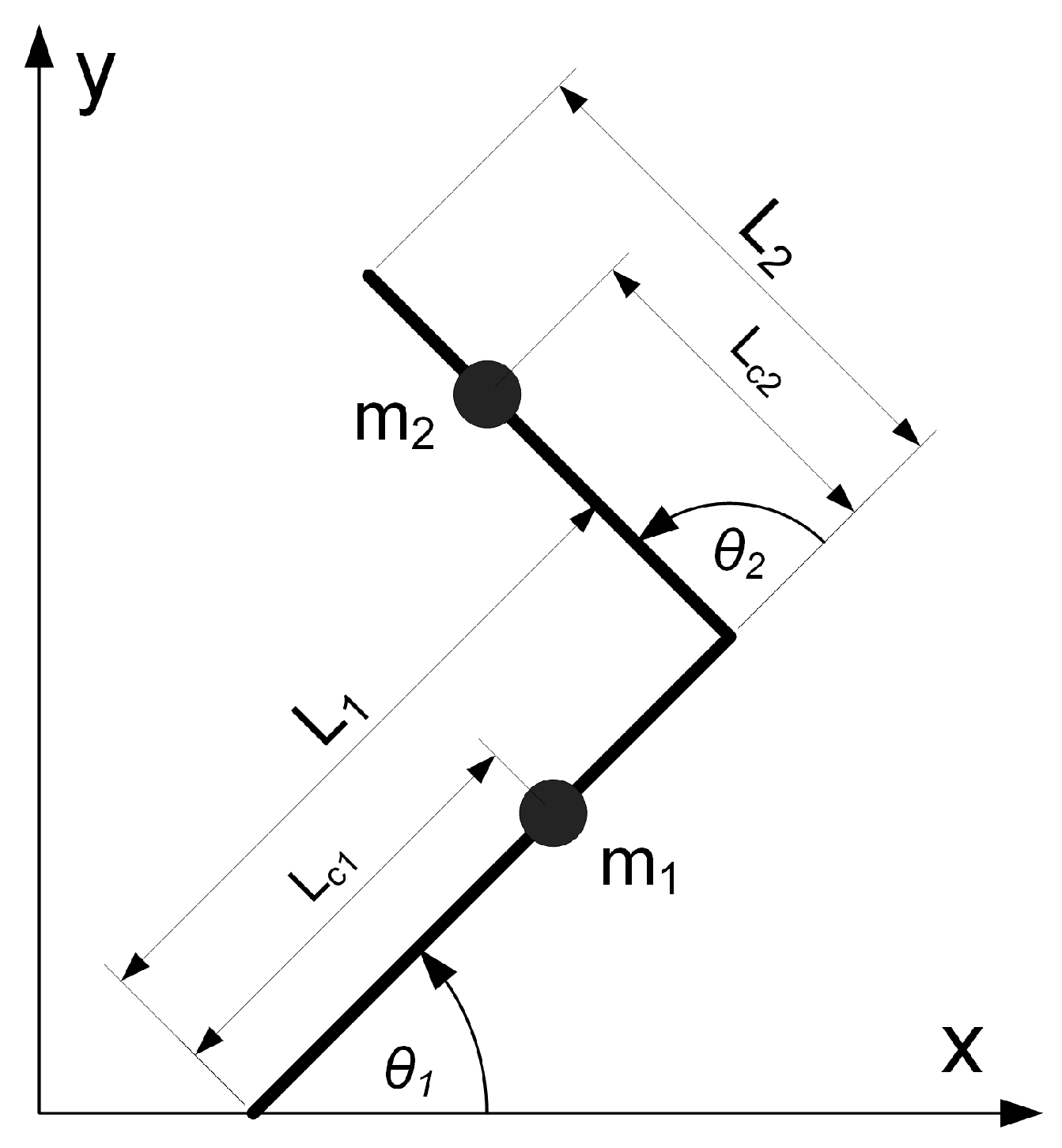
2. Model
3. Control Problem
3.1. Control Algorithm Based on Partial Linearization
3.1.1. Zero Dynamics
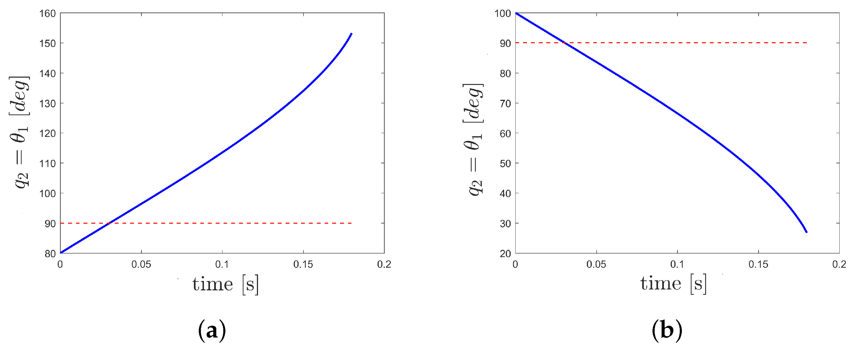
3.1.2. Avoiding of Singular Points
3.2. Linear Controller
4. Simulation and Experimental Results
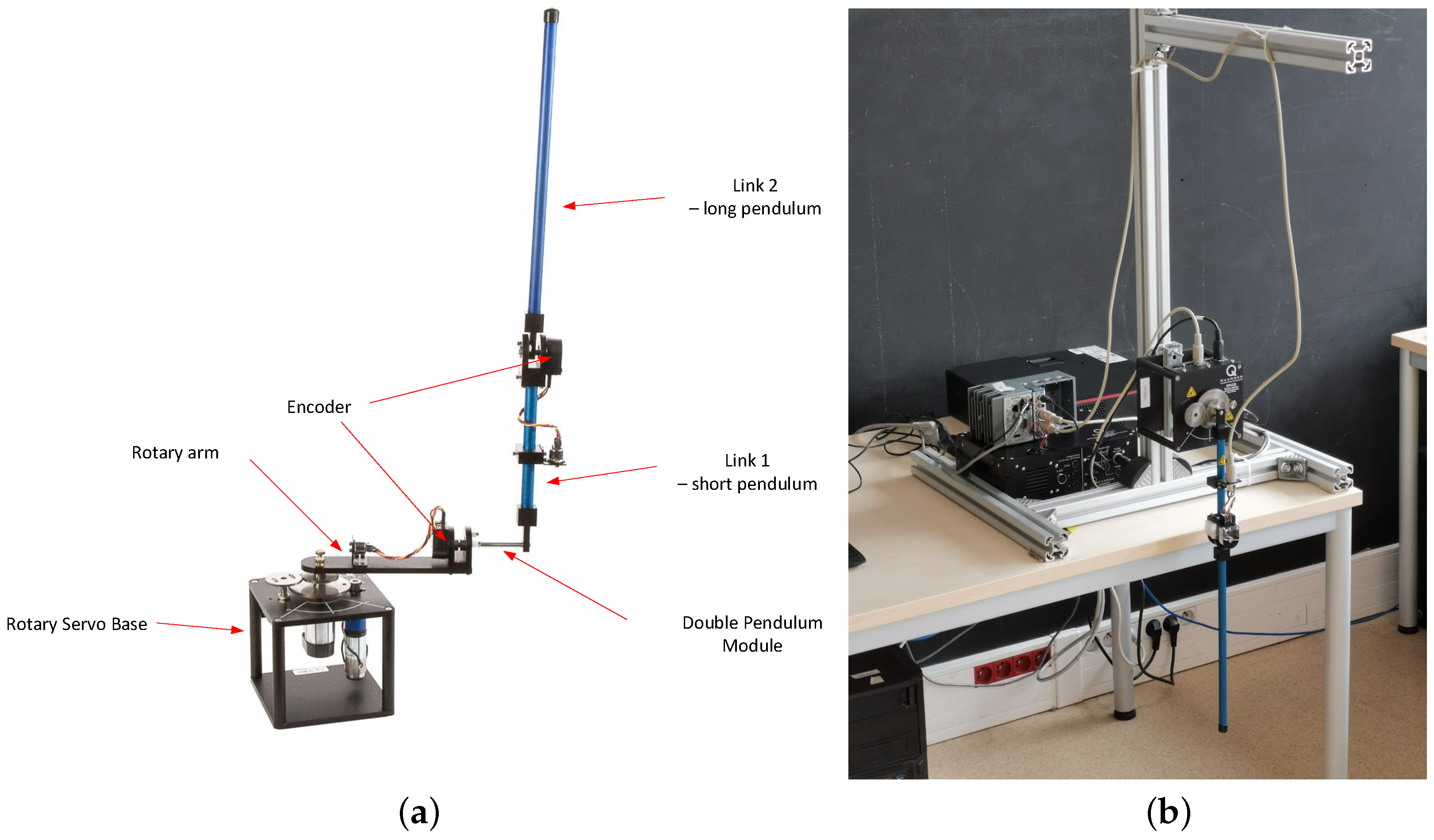
4.1. Characteristics of the Laboratory Pendubot-Like System
4.2. Simulation Procedure
- Algorithm 1— is defined using the collocated linearization;
- Algorithm 2— is defined using the non-collocated linerization;
- Algorithm 3— is defined based on the maximum partial linearization approach described in this paper.
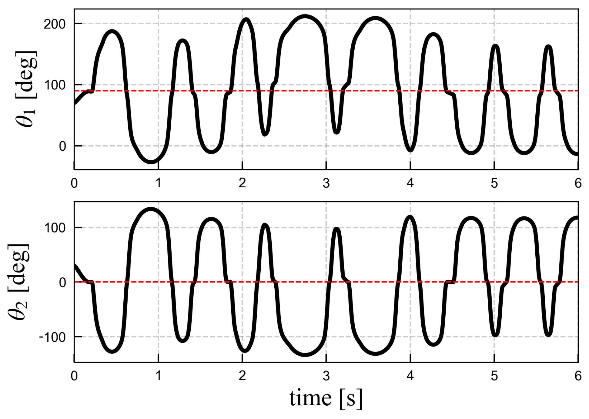
4.3. Experimental Results
5. Conclusions
Author Contributions
Funding
Acknowledgments
Conflicts of Interest
References
- Fantoni, I.; Lozano, R.; Spong, M. Energy based control of the Pendubot. IEEE Trans. Autom. Control 2000, 45, 725–729. [Google Scholar] [CrossRef] [Green Version]
- Spong, M.W. The swing up control problem for the Acrobot. IEEE Control Syst. Mag. 1995, 15, 49–55. [Google Scholar] [CrossRef] [Green Version]
- Spong, M.W. Partial feedback linearization of underactuated mechanical systems. In Proceedings of the IEEE/RSJ International Conference on Intelligent Robots and Systems (IROS’94), Munich, Germany, 12–16 September 1994; Volume 1, pp. 314–321. [Google Scholar]
- Xin, X.; Kaneda, M. New analytical results of the energy based swinging up control of the Acrobot. In Proceedings of the 2004 43rd IEEE Conference on Decision and Control (CDC) (IEEE Cat. No.04CH37601), Nassau, Bahamas, 14–17 December 2004; Volume 1, pp. 704–709. [Google Scholar] [CrossRef]
- Spong, M.; Block, D. The Pendubot: A mechatronic system for control research and education. In Proceedings of the 1995 34th IEEE Conference on Decision and Control, New Orleans, LA, USA, 13–15 December 1995; Volume 1, pp. 555–556. [Google Scholar] [CrossRef]
- Åström, K.; Furuta, K. Swinging up a pendulum by energy control. Automatica 2000, 36, 287–295. [Google Scholar] [CrossRef] [Green Version]
- Li, J.H. Dual fuzzy PD control of DSP-based pendubot. In Proceedings of the 2011 8th Asian Control Conference (ASCC), Kaohsiung, Taiwan, 15–18 May 2011; pp. 641–646. [Google Scholar]
- Orlov, Y.; Aguilar, L.; Acho, L. Model Orbit Robust Stabilization (MORS) of Pendubot with Application to Swing up Control. In Proceedings of the 44th IEEE Conference on Decision and Control, Seville, Spain, 15 December 2005; pp. 6164–6169. [Google Scholar] [CrossRef]
- Ramírez-Neria, M.; Sira-Ramírez, H.; Garrido-Moctezuma, R.; Luviano-Juárez, A.; Gao, Z. Active Disturbance Rejection Control for Reference Trajectory Tracking Tasks in the Pendubot System. IEEE Access 2021, 9, 102663–102670. [Google Scholar] [CrossRef]
- Toan, T.V.; Ha, T.T.; Do, T.V. Hybrid control for swing up and balancing pendubot system: An experimental result. In Proceedings of the 2017 International Conference on System Science and Engineering (ICSSE), Ho Chi Minh City, Vietnam, 21–23 July 2017; pp. 450–453. [Google Scholar] [CrossRef]
- Sellami, S.; Mamedov, S.; Khusainov, R. A ROS-based swing up control and stabilization of the Pendubot using virtual holonomic constraints. In Proceedings of the 2020 International Conference Nonlinearity, Information and Robotics (NIR), Innopolis, Russia, 3–6 December 2020; pp. 1–5. [Google Scholar] [CrossRef]
- Xu, T.; Fan, J.; Fang, Q.; Wang, S.; Zhu, Y.; Zhao, J. A Novel Virtual Sensor for Estimating Robot Joint Total Friction Based on Total Momentum. Appl. Sci. 2019, 9, 3344. [Google Scholar] [CrossRef] [Green Version]
- Deng, M.; Kubota, S. Nonlinear Control System Design of an Underactuated Robot Based on Operator Theory and Isomorphism Scheme. Axioms 2021, 10, 62. [Google Scholar] [CrossRef]
- Kozłowski, K.; Pazderski, D.; Parulski, P.; Bartkowiak, P. Stabilization of a 3-Link Pendulum in Vertical Position. In Advanced, Contemporary Control; Bartoszewicz, A., Kabzinski, J., Kacprzyk, J., Eds.; Springer International Publishing: Cham, Switzerland, 2020; pp. 651–662. [Google Scholar]
- Li, S.; Moog, C.; Respondek, W. Maximal feedback linearization and its internal dynamics with applications to mechanical systems on R4. Int. J. Robust Nonlinear Control 2019, 29, 2639–2659. [Google Scholar] [CrossRef]
- Bartkowiak, P. Control of 2 DOF Planar Underactuated Manipulator. Master’s Thesis, Poznan University of Technology, Poznań, Poland, 2019. (In Polish). [Google Scholar]
- Xin, X.; Kaneda, M.; Oki, T. The Swing Up Control for the Pendubot Based on Energy Control Approach. IFAC Proc. Vol. 2002, 35, 461–466. [Google Scholar] [CrossRef] [Green Version]
- Khalil, H. Nonlinear Systems; Prentice Hall: Upper Saddle River, NJ, USA, 1996. [Google Scholar]
- Quanser. Rotary Double Inverted Pendulum. Available online: www.quanser.com/products/rotary-double-inverted-pendulum/ (accessed on 18 August 2021).
- Abdel-Malek, K.; Arora, J. Human Motion Simulation: Predictive Dynamics; Academic Press in an Imprint of Elsevier: Waltham, MA, USA; San Diego, CA, USA; London, UK, 2013. [Google Scholar]


| Link | Mass | Length | Centre of Mass | Inertia |
|---|---|---|---|---|
| i | [kg] | [m] | [m] | [] |
| 1 | 0.097 | 0.20 | 0.1635 | 0.0069 |
| 2 | 0.127 | 0.3365 | 0.1778 | 0.0048 |
| Algorithm 1 | Algorithm 2 | Algorithm 3 | |
|---|---|---|---|
| mean | 413.87 | 100.71 | 144.44 |
| 639.50 | 57.95 | 195.97 | |
| mean | 48.55 | 55.11 | 115.90 |
| 28.48 | 27.56 | 119.88 |
Publisher’s Note: MDPI stays neutral with regard to jurisdictional claims in published maps and institutional affiliations. |
© 2021 by the authors. Licensee MDPI, Basel, Switzerland. This article is an open access article distributed under the terms and conditions of the Creative Commons Attribution (CC BY) license (https://creativecommons.org/licenses/by/4.0/).
Share and Cite
Parulski, P.; Bartkowiak, P.; Pazderski, D. Evaluation of Linearization Methods for Control of the Pendubot. Appl. Sci. 2021, 11, 7615. https://doi.org/10.3390/app11167615
Parulski P, Bartkowiak P, Pazderski D. Evaluation of Linearization Methods for Control of the Pendubot. Applied Sciences. 2021; 11(16):7615. https://doi.org/10.3390/app11167615
Chicago/Turabian StyleParulski, Paweł, Patryk Bartkowiak, and Dariusz Pazderski. 2021. "Evaluation of Linearization Methods for Control of the Pendubot" Applied Sciences 11, no. 16: 7615. https://doi.org/10.3390/app11167615
APA StyleParulski, P., Bartkowiak, P., & Pazderski, D. (2021). Evaluation of Linearization Methods for Control of the Pendubot. Applied Sciences, 11(16), 7615. https://doi.org/10.3390/app11167615