Abstract
A new methodology, the hybrid learning system (HLS), based upon semi-supervised learning is proposed. HLS categorizes hyperspectral images into segmented regions with discriminative features using reduced training size. The technique utilizes the modified breaking ties (MBT) algorithm for active learning and unsupervised learning-based regressors, viz. multinomial logistic regression, for hyperspectral image categorization. The probabilities estimated by multinomial logistic regression for each sample helps towards improved segregation. The high dimensionality leads to a curse of dimensionality, which ultimately deteriorates the performance of remote sensing data classification, and the problem aggravates further if labeled training samples are limited. Many studies have tried to address the problem and have employed different methodologies for remote sensing data classification, such as kernelized methods, because of insensitiveness towards the utilization of large dataset information and active learning (AL) approaches (breaking ties as a representative) to choose only prominent samples for training data. The HLS methodology proposed in the current study is a combination of supervised and unsupervised training with generalized composite kernels generating posterior class probabilities for classification. In order to retrieve the best segmentation labels, we employed Markov random fields, which make use of prior labels from the output of the multinomial logistic regression. The comparison of HLS was carried out with known methodologies, using benchmark hyperspectral imaging (HI) datasets, namely “Indian Pines” and “Pavia University”. Findings of this study show that the HLS yields the overall accuracy of {99.93% and 99.98%}Indian Pines and {99.14% and 99.42%}Pavia University for classification and segmentation, respectively.
1. Introduction
Hyperspectral imaging (HI), introduced at National Aeronautics and Space Administration (NASA)’s Jet Propulsion Laboratory [1], is a system that consists of spatial in conjunction with spectral coordinates forming a hyperspectral cube. This imaging system is being used in diverse fields viz. security control [2], pharmaceutical analysis [3], agriculture quality [4], biomedical sciences [5], and many others. Hyperspectral remote sensing is an active analysis in the field of the land area [6] and recent examples of remote sensing is an airborne visible/infrared imaging spectrometer (AVIRIS) sensor [7], operational at the NASA Propulsion Laboratory. Nowadays, AVIRIS sensors are capturing more than 200 spectral bands against each pixel, carrying huge information about an object, which is much better than previous primitive sensors [8]. One of the most popular and important areas of processing hyperspectral remote sensing is classification. Here the task is to classify each pixel of the hyperspectral image by assigning a label for generating a thematic land-cover map [9]. In this regard, several studies have been carried out in the last decade by applying a variety of machine learning and image processing methods to extract useful information from hyperspectral data [10].
Hyperspectral image analysis can classify the materials in an area under observation in a better way based on the huge spectral information obtained but at the cost of high spectral dimensionality. On the contrary, high dimensionality brings along with it the curse of the dimensionality problem that destroys classification performance (Feng et al., 2017). Furthermore, the Hughes effect arises due to high dimensionality in the hyperspectral data that pose critical problems for supervised learning methods to perform effectively [10,11], and sometimes one pixel contains a lot of spectral information with spatial information lost. In a similar manner, sometimes, a single channel contains spatial information, but spectral information is lost [12,13]. Attempts have been made to address the problem, such as that by Fauvel et al. [14]. They described all the details about spectral-spatial advancements in the scenario of classification.
Two kinds of features are mainly extracted from remote sensing data for classification [15].
- First, the main feature is that spectral information lies in the third dimension against each pixel entry in a data cube, and it can be extracted for the exploitation of linear separability of the classes. Numerous methods have been developed for extraction, such as independent component analysis [16], linear spectral unmixing [17,18], and maximum noise fraction [19].
- The second information is the spatial information for which numerous methods have been used, such as manifold regularization [20,21], kernel methods [22,23], and morphological analysis [13,24].
During the last decade, different conventional machine learning methods have used a large number of training samples for training over data [25,26]. In remote sensing datasets, normally, a limited number of reliable samples are available. Wang et al. [27] addressed this issue so that all labeled samples are not used in the training process. Wang et al. suggested that prominent samples should be selected only for training, based on active learning (AL), so that the maximum number of samples would be available during the testing phase [28,29], leading to an agreeable generalization accuracy. Li et al. [30,31,32] have shown that there are different ways to use AL for remote sensing, namely random selection (RS), maximum entropy (ME), mutual information (MI) [33,34], breaking ties (BT) [35], and modified breaking ties (MBT) [36].
Bruzzone et al. showed a significant improvement in classification with extracted spectral and spatial features from the dataset. Better classification is achieved when reliable samples are being used in training [37]. Samples usually are very expensive with regard to time and cost, and it is not so common to utilize this type of large ground truth information. Schölkopf and Smola [22] addressed the issue that kernelized methods that are insensitive towards the utilization of large dataset information due to the curse of dimensionality. Good generalization capability can be achieved using different kernelized methods with even a limited number of reliable training samples [23,38]. There exist numerous methods for the use of large ground truth information such as SVM [39], semi-supervised SVM [40], multinomial logistic regression (MLR) [41], partial least squares regression [42], and artificial neural networks [43]. In both spectral and spatial information, researchers have started to employ neural networks such as densely connected multiscale attention networks [44], end-to-end fully convolutional segmentation networks [45], and convolutional neural networks (CNN) with random forest [46] and Ghostnet [47].
In this work, a hybrid learning system (HLS) is introduced and tested that categorizes hyperspectral images into segmented regions with discriminative features using reduced training size. It is based on a semi-supervised learning approach, using an MBT algorithm for AL and multinomial logistic regression for unlabeled HI data categorization. For the training phase, a smaller number of samples are selected using the AL method (modified breaking ties). HLS is a combination of supervised and unsupervised training with generalized composite kernels generating posterior class probabilities for classification. Finally, Markov random fields are used to get the best segmentation label by using class prior labels from the output of the multinomial logistic regression. The proposed methodology is tested by comparing it with known methodologies for hyperspectral image classification and segmentation. Two benchmark HI datasets, namely “Indian Pines” and “Pavia University” are used for experimentation. The article is organized as follows: Section 2 describes the Methodology, including dataset description with processes and stages involved in HI; Results and Discussion are reported in Section 3 with a comprehensive comparison with existing researchers’ work, and Section 4 provides the concluding remarks.
2. Materials and Methods
The hyperspectral image classification and segmentation tasks are related problems. The goal of image classification is to assign a class label to each pixel in the hyperspectral image whilst segmentation refers to the partition of the set of image pixels into the collection of sets. These sets are declared regions where the pixels in each set are close to each other in some sense. Notably, the term classification is used when there is no spatial information taken into account. On the other hand, the term segmentation is used when spatial prior information is being considered. Let P is a set of n pixels of HI as given by . Similarly, where M is a set of integers consisting of dataset labels. Further, let X is a set of d-dimensional vectors of image pixels represented as . Y is shown below as the set of labels for a dataset . The purpose behind this problem formulation is to classify each pixel and assign them their best label and also segment them into different regions based on labels for pixel [28]. The flow chart for the proposed methodology, namely the hybrid learning system (HLS), is presented in Figure 1. After training on AL-based samples, posterior probabilities were generated by a generalized composite kernels algorithm. On these probabilities, the maxim-a-posteriori algorithm was employed to find the best class probability/label against each training sample. On these classification labels, an α-expansion algorithm is run to generate the segmentation map. Generally in classification, spectral–spatial kernels are computed over a sample with its immediate and farther neighbors to assign it the probabilities, but in segmentation, the best label is assigned based on immediate neighbors. We have used two datasets to conduct our experimentation. Initially, each dataset is passed to extended attribute profiles (EAPs) for the components’ selection. After selecting the components, the MBT algorithm was applied for AL and multinomial logistic regression is applied for unlabeled HI data. Then, the output from multinomial logistic regression is used for segmentation. The method is iterated over ten Monte Carlo runs to get optimal results.
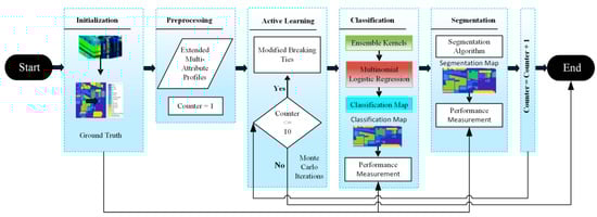
Figure 1.
The hybrid learning system for classification and segmentation of the HI landscape dataset.
2.1. Datasets
In this study, two sets of landscape images were used for HI-based classification: the “Indian Pines” and “Pavia University” datasets. The AVIRIS sensors were used to acquire the Indian Pines dataset collected over the Northwestern Indiana region. It is 3D-data where the first two dimensions, 145 × 145, represent spatial information while the third one corresponds to 202 spectral channels wavelengths ranges from 400–2500 nm. Each pixel has a spectral resolution of 10 nm and represents an area of 20 × 20 m2. There are 16 classes in this dataset with 10,366 instances. Although the dataset is imbalanced, the proposed methodology uses fewer instances for training sessions, thereby relieving the inherent effect of the unbiased nature of the dataset. For regions visualization, an image of spectrum for band (150) in grayscale is shown in Figure 2a.
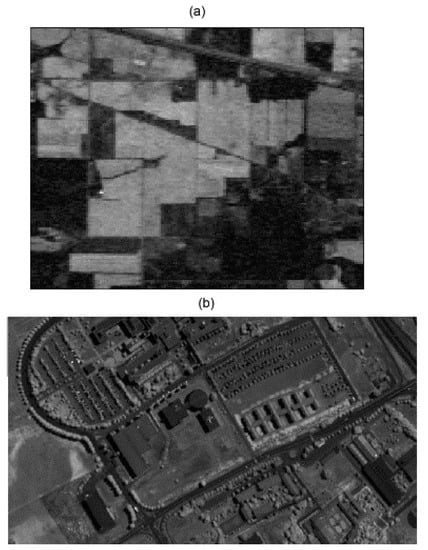
Figure 2.
Gray level representation of single bands for the HI dataset, (a) band number 150 of the Indian Pines dataset, and (b) band number 90 of the Pavia University dataset.
The Pavia University dataset has been acquired using a ROSIS sensor by capturing the Pavia University, Italy region. It consists of 3D-data where the first two dimensions, 610 × 340, express the spatial resolution while the third dimension represents 103 spectral wavelength channels in the range 430–860 nm. Each pixel has a geometric resolution of 1.3 m. This dataset has 9 classes and 207,400 instances. For regions visualization, the spectral band, namely number 90, in the grayscale channel has been shown in Figure 2b.
2.2. Multinomial Logistic Regression (MLR)
The set represents regressors (logistic) and is the rth class set of regressors [28]. The posterior-class probabilities, as well as regressors, are calculated by the MLR model as given by
The important point here is that the value of because the density is not dependent on translation on the regressor . The function where k represents the total number of feature vectors. The f (linear/nonlinear) is given by , where represents the th element of . The kernels are given by , here, and some kind of symmetry also exists in the function F. Parameters are mapped in a nonlinear manner. For this, radial basis function has been employed represented as:
It is important to learn the class densities for regressors’ estimation. The class densities are estimated using labeled and unlabeled samples, where represents labeled samples (small set) and represents unlabeled samples (large set). Posterior density using labeled as well as unlabeled data is given by:
where represents set of labels in , represents feature vectors set in , and represents labeled as well as unlabeled sets of samples. The maximum-a-posteriori (MAP) estimation for regressors is computed as given by , where
Here, is the log-likelihood function over c provided the samples have labels and where the latter works as prior information over c. Further, the Gaussian prior is given by , where is a precision matrix and is built in such a way that the regressors c is promoted by the density . This leaves samples in the class having similar features f(x) (either labeled or unlabeled). It is important here to compute the distance between features.
2.3. Regression Estimator Using MAP
EM-algorithm is used iteratively for computation of MAP for c. The general forms of expectation and maximization steps are given by and , where vector , is a scaling factor for i = 1, …, N-1, representing missing variables and is the set having instances of the labeled and unlabeled dataset. Now we can compute the Gaussian prior by using the sequence of where t = 1, 2, … is an increasing function.
2.4. EMAPs with Spatial Information
The morphological profiles (MPs) and attribute profiles (APs) were determined to merge the spatial and spectral information to assist classification. The attribute filters (AFs) for computing APs, using gray level images were defined in a mathematical morphological framework that operated by combining components at different threshold levels. The filtering operation applied on grayscale images with given threshold values checks whether the current component is going to merge lower gray levels or otherwise. Here, merging of components to lower gray level means thinning, and higher gray level means thickening. In this technique, the entire feature (spectral band) extracted from the original pixel was not considered, and several principal components are taken for this technique and the remaining components are ignored. This yields extended attribute profiles (EAPs). In this research work, the first three principal components are considered that hold most of the associated variance. The stacked EAPs, using different types of attributes, are called extended multi-attribute profiles (EMAP). These are used to enhance extractability related to spatial features from a landscape.
2.5. Approach of Generalized Composite Kernels
Generalized composite kernels (GCKs) are used for spectral-spatial classification. In the proposed methodology, stacked cross-kernels are used as: and the input function is given by:
Therefore, MAP estimation for may be written as:
Here, we have used variable splitting and augmented Lagrangian optimization technique to deal with large kernel sizes for improved computational performance [30].
2.6. Isotropic Multi-Level Logistic (MLL) Prior
A logical approach for image segmentation is that the contiguous pixels mostly lie in the same class. This approach has been exploited here with background information where image modeling, isotropic multi-level logistic (MLL) prior has been used. Piecewise-smooth segmentations are encouraged by this prior by using Markov random fields (MRF) where the Gibbs energy is computed. Therefore, the prior model for segmentation is given by:
Here, z is a normalizing factor and is called prior potential and k is a set of cliques over the image. The potential over cliques is computed by:
It is clear from Equation (8) that the neighboring pixels have the same labels. The Equation (7) becomes flexible by introducing and > 0 and it is given by:
where is controlling the level of smoothness and determines the higher probability towards label assignment.
2.7. Performance Measures
The performance measures for classification as well as segmentation for HLS are overall- and average- accuracies, including Kappa statistics. We have calculated the Overall Accuracy (OA), Average Accuracy (AA) [28], and Kappa () statistics [48] using the following relationships as given by , where represents true predicted instances and N is the total number of actual instances in the experiment. Similarly, , where represents true predicted instances of the ith class, is the number of actual instances of ith class while L indicates the total number of classes in the experiment, and , where represents the actual observed agreement and represents the chance agreement. This measure is used to test inter-rater reliability. It shows the reliability of the data collected in the experimentation having the right representation of measured variables [49].
3. Results and Discussion
This section focuses on the results of experiments performed for the classification and segmentation of the HI scans. Firstly, a brief description of the experimental setup is provided followed by the experimental results with a discussion of the proposed methodology. Finally, a comprehensive comparison with the existing techniques is made at the end.
3.1. Experimental Setup
The experimentation was carried out using a Dell Alien machine, Intel (R) Core (TM) i7—7700 HQ CPU @ 2.80 GHz, having 32 GB RAM. The operating system used was Microsoft Windows with open source software and library programs.
Numerous parameters for computing EMAPs have been found, concerning mean value 2.5–10%, standard deviation value 2.5%, and threshold range is (200–500). The experiment is performed by running independent Monte Carlo iterations 10 times and has empirically found the optimum number of samples to generate outstanding results. Before and after this sampling threshold, accuracy suffered degradation.
After classification, the MAP estimation was passed to the segmentation algorithm, where the MLL algorithm was used for segregating the classes. Here, different accuracy measures were tabulated for each class corresponding to AL methods, namely RS, ME, MI, MB, and MBT. The classification results in terms of overall for all these AL techniques, in the case of the Indian Pines dataset, varied from 98.13 to 99.93%. The Indian Pines ground truth is pictorially shown in Figure 3a, while the classification and segmentation pictogram are shown in Figure 3b,c, respectively. These results may be compared subjectively based on the perceptual information within the original images shown in Figure 3a. The quantitative performance of classification and segmentation is illustrated in Table 1 and Table 2 for Indian Pines. The results were outstanding for classification for the Indian Pines dataset as shown in Table 1, having OA, AA, and kappa statistics as 99.93, 99.86, and 99.84%, respectively. Whereas for segmentation, each of the performance measures (OA, AA, and kappa) have been found as 99.98%, as shown in Table 2. For classification, most of the past methods were based on the exploitation of spectral information [50]. Researchers having similar thoughts relied on the fact that single spectral information is enough for better classification [14,51,52]. These extracted spectral features, representing independent characteristics, were fed to the classifier without using the spatial information in contiguous pixel dependency. Tarabalka et al. [53] addressed the solution of this issue, that exploitation of the spectral information only is not enough for classification. Spatial information should incorporate with spectral information for better results [15,30,32,54,55,56,57]. Li et al. [28] have also shown the importance of spatial information with spectral information. Jain et al. [58] have elaborated hyperspectral image classification with a combination of SVM using self-organizing maps (SOMs). This technique is divided into two phases; the first one is based on the training of the SVM using SOM, while the second is based on the calculation of probabilities by finding the interior and exterior pixels, so the best label should be decided based on an optimal threshold. The comparison of existing techniques using the Indian Pines datasets is shown in Table 3 (Section 3.2).
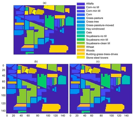
Figure 3.
(a) Ground truth map (dimensions: 145 × 145), (b) classification map for the Indian Pines dataset using HLS (dimensions: 145 × 145), and (c) segmentation map for the Indian Pines dataset using HLS (dimensions: 145 × 145).

Table 1.
Classification accuracy of Indian Pines dataset (class-wise) on 10 independent repetitions using active learning techniques.
Table 2.
Segmentation accuracy of the Indian Pines dataset (class-wise) using HLS.
Table 3.
Comparison of classification and segmentation accuracies of the Indian Pines dataset (class-wise) on 10 repetitions using 5 training samples of each class.
In the Pavia University experiment, the pictorial representation of ground truth, classification and segmentation landscapes of our proposed methodology are shown in Figure 4a–c. The representation of nine classes, i.e., asphalt, bare soil, bitumen, bricks, gravel, meadows, metal sheets, shadows, and trees, have been used to produce the ground truth. Every class with separate color can be seen after the application of the algorithm. Similar to the previous experimentation, empirically found number of samples using different active learning algorithms are computed by ten independent Monte Carlo runs. The classification results of each class are shown in Table 4 as OA, AA, and k-statistics as 99.14, 98.56, and 99.01%, respectively. The segmentation results in tabular form are illustrated in Table 5 for different active learning strategies. The segmentation results of the proposed methodology for the Pavia University dataset are: (OA, AA, and k-statistics as 99.42, 99.29, and 99.28%, respectively).
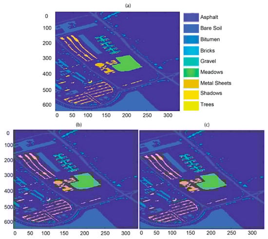
Figure 4.
(a) Ground truth map (dimensions: 610 × 340), (b) classification map for the Pavia University dataset using HLS (dimensions: 610 × 340), and (c) segmentation map for the Pavia University dataset using HLS (dimensions: 610 × 340).
Table 4.
Classification accuracy of the Pavia University dataset (class-wise) on 10 independent repetitions using HLS.
Table 5.
Segmentation accuracy of the Pavia University dataset (class-wise) using HLS.
The existing models [28,30,31,32] were tested on freely available datasets, and further, the results were compared with the proposed framework (Table 3 and Table 6) using five samples from each class (Table 1 and Table 4).
Table 6.
Comparison of classification and segmentation accuracies of the Pavia University dataset (class-wise) on 10 repetitions using 5 training samples of each class.
3.2. Comparison with Existing Techniques
At the end of the experimentation phase, a comprehensive comparison of classification and segmentation was conducted on existing methodologies. The comparison was performed on five training instances for the Indian Pines and Pavia University datasets, respectively, as shown in Table 3 and Table 6. It can be noted that RS, ME, MI, and BT showed relatively poor performance as compared to MBT. This was attributed to the fact that former techniques usually select samples from complex areas, having the least confidence, which causes difficulty in learning procedure [36]. In comparison, the MBT outperformed as compared to the other active learning techniques, as it selected only those samples that were lying in the vicinity of high-density samples in each class.
Mura et al. [59] introduced morphological attribute profiles (MAPs). Morphological profile filters are used to extract structural information. These calculated profiles are more flexible and lead to better investigation of the contextual information by using different morphological attribute transformations. Makantasis et al. [60] employed a convolutional neural network to encode spectral and spatial information. The output is fed to a multi-layer perceptron for classification. The overall accuracy of 98% was achieved when the author used 30 samples of the Indian Pines dataset with deep neural networks. The relatively low performance by using even higher number of samples is the inherent capability of deep learning strategies as given in [61]. The remarkable segmentation results of the proposed methodology were owed to the use of well-classified data before the segmentation phase. The algorithm consumed relatively more resources for computation as compared to conventional solutions. Similarly, a semi-supervised approach for segmentation was introduced by Li et al. [42] in which the posterior class probabilities were calculated by MLR algorithm. Maximum-a-posteriori (MAP) was computed on this output to calculate the best classification label. The multi-level logistic (MLL) algorithm was then employed with Markov random fields (MRF) to compute the segmentation [44,45]. Moreover, MRF works on the model of Gibbs energy to calculate the best segmentation label, based on current pixel potential for the neighboring pixels, to decide whether this pixel belongs to the current region or not [46,47].
4. Conclusions
There always exists information corresponding to each channel (wavelength) during the acquisition process in hyperspectral imaging (HI). Since diffuse scattering and reflection are specific to material dependence, this dimension has enormous applications in biomedical, geography, defense, and chemistry. In this paper, a novel methodology is introduced that is called hybrid learning system (HLS), which categorizes hyperspectral images into segmented regions with discriminative features using reduced training size. HLS is a semi-supervised learning approach using active learning, a supervised learning technique, and unsupervised learning-based MLR for classification and segmentation of HI. The proposed method outperformed with a fewer number of training instances. For merged spatial and spectral information, EMAPS are computed first for each dataset to give improved classification results. Generalized composite kernels have been used in the MLR algorithm for classification to produce the posterior class probabilities against each instance for better segmentation of landscapes. The comparison of work has been carried out using benchmark datasets, i.e., “Indian Pines” and “Pavia University” with known methodologies. The HLS based HI has been found to yield an overall accuracy of {99.93% and 99.98%} Indian Pines and {99.14% and 99.42%}Pavia University for classification and segmentation, respectively.
Author Contributions
Conceptualization, S.A.Q., S.T.H.S., A.u.R. and A.A. (Arslan Amjad); methodology, S.A.Q., S.T.H.S., A.u.R., M.R. and A.A. (Amal Alqahtani); software, S.A.Q. and S.T.H.S.; validation, S.A.Q., S.T.H.S., S.A.H.S., A.u.R., A.A. (Amal Alqahtani), D.A.B., A.A. (Arslan Amjad), A.A.M., M.U.K., M.R.I.F. and M.R.; formal analysis, S.A.Q., S.T.H.S., S.A.H.S., A.u.R., A.A. (Amal Alqahtani), D.A.B., A.A. (Arslan Amjad), A.A.M., M.U.K., M.R.I.F. and M.R.; investigation, S.A.Q., S.T.H.S., S.A.H.S., A.u.R., A.A. (Arslan Amjad), D.A.B., A.A. (Amal Alqahtani), A.A.M., M.U.K., M.R.I.F. and M.R.; resources, S.A.Q. and S.T.H.S.; data curation, S.A.Q., S.T.H.S., S.A.H.S., A.u.R., A.A. (Arslan Amjad), D.A.B., A.A. (Amal Alqahtani), A.A.M., M.U.K., M.R.I.F. and M.R.; writing—original draft preparation, S.A.Q. and S.T.H.S.; writing—review and editing, S.A.Q., S.T.H.S., S.A.H.S., A.u.R., A.A. (Arslan Amjad), D.A.B., A.A. (Amal Alqahtani), A.A.M., M.U.K., M.R.I.F. and M.R.; visualization, S.A.Q., S.T.H.S., S.A.H.S., A.u.R., A.A. (Arslan Amjad), D.A.B., A.A. (Amal Alqahtani), A.A.M., M.U.K., M.R.I.F. and M.R.; supervision, S.A.Q.; project administration, S.A.Q.; funding acquisition, D.A.B. and A.A. (Amal Alqahtani). All authors have read and agreed to the published version of the manuscript.
Funding
The authors acknowledged the APC contribution by the Deanship of Preparatory Year and Supporting Studies, Imam Abdulrahman Bin Faisal University P.O. Box 1982, Dammam 34212, Saudi Arabia.
Data Availability Statement
Not applicable.
Acknowledgments
The authors acknowledged the APC contribution by the Deanship of Preparatory Year and Supporting Studies, Imam Abdulrahman Bin Faisal University P.O. Box 1982, Dammam 34212, Saudi Arabia. We would like to thank the anonymous reviewers for their suggestions, comments and constructive input.
Conflicts of Interest
The authors declare no conflict of interest.
References
- Goetz, A.F.; Vane, G.; Solomon, J.E.; Rock, B.N. Imaging spectrometry for earth remote sensing. Science 1985, 228, 1147–1153. [Google Scholar] [CrossRef]
- Yuen, P.W.T.; Richardson, M. An introduction to hyperspectral imaging and its application for security, surveillance and target acquisition. Imaging Sci. J. 2010, 58, 241–253. [Google Scholar] [CrossRef]
- Roggo, Y.; Edmond, A.; Chalus, P.; Ulmschneider, M. Infrared hyperspectral imaging for qualitative analysis of pharmaceutical solid forms. Anal. Chim. Acta 2005, 535, 79–87. [Google Scholar] [CrossRef]
- Dale, L.M.; Thewis, A.; Boudry, C.; Rotar, I.; Dardenne, P.; Baeten, V.; Pierna, J.A.F. Hyperspectral imaging applications in agriculture and agro-food product quality and safety control: A review. Appl. Spectrosc. Rev. 2013, 48, 142–159. [Google Scholar] [CrossRef]
- Lu, G.; Fei, B. Medical hyperspectral imaging: A review. J. Biomed. Opt. 2014, 19, 010901. [Google Scholar] [CrossRef] [PubMed]
- Qiao, T.; Yang, Z.; Ren, J.; Yuen, P.; Zhao, H.; Sun, G.; Marshall, S.; Benediktsson, J.A. Joint bilateral filtering and spectral similarity-based sparse representation: A generic framework for effective feature extraction and data classification in hyperspectral imaging. Pattern Recognit. 2018, 77, 316–328. [Google Scholar] [CrossRef] [Green Version]
- Green, R.O.; Eastwood, M.L.; Sarture, C.M.; Chrien, T.G.; Aronsson, M.; Chippendale, B.J.; Faust, J.A.; Pavri, B.E.; Chovit, C.J.; Solis, M.; et al. Imaging spectroscopy and the airborne visible/infrared imaging spectrometer (AVIRIS). Remote Sens. Environ. 1998, 65, 227–248. [Google Scholar] [CrossRef]
- Thompson, D.R.; Boardman, J.W.; Eastwood, M.L.; Green, R.O. A large airborne survey of Earth’s visible-infrared spectral dimensionality. Opt. Express 2017, 25, 9186. [Google Scholar] [CrossRef] [Green Version]
- Shaw, G.; Manolakis, D. Signal processing for hyperspectral image exploitation. IEEE Signal Process. Mag. 2002, 19, 12–16. [Google Scholar] [CrossRef]
- Plaza, A.; Benediktsson, J.A.; Boardman, J.W.; Brazile, J.; Bruzzone, L.; Camps-Valls, G.; Chanussot, J.; Fauvel, M.; Gamba, P.; Gualtieri, A. Recent advances in techniques for hyperspectral image processing. Remote Sens. Environ. 2009, 113, S110–S122. [Google Scholar] [CrossRef]
- Borges, J.S.; Bioucas-Dias, J.M.; Marcal, A.R. Bayesian hyperspectral image segmentation with discriminative class learning. IEEE Trans. Geosci. Remote Sens. 2011, 49, 2151–2164. [Google Scholar] [CrossRef]
- Shah, S.T.H.; Javed, S.G.; Majid, A.; Shah, S.A.H.; Qureshi, S.A. Novel classification technique for hyperspectral imaging using multinomial logistic regression and morphological profiles with composite kernels. In Proceedings of the IEEE International Bhurban Conference on Applied Sciences and Technology, IBCAST 2019, Nathiagalli, Pakistan, 8–12 January 2019; pp. 419–424. [Google Scholar]
- Benediktsson, J.A.; Palmason, J.A.; Sveinsson, J.R. Classification of hyperspectral data from urban areas based on extended morphological profiles. IEEE Trans. Geosci. Remote Sens. 2005, 43, 480–491. [Google Scholar] [CrossRef]
- Fauvel, M.; Tarabalka, Y.; Benediktsson, J.A.; Chanussot, J.; Tilton, J.C. Advances in Spectral-Spatial Classification of Hyperspectral Images. Proc. IEEE 2013, 101, 652–675. [Google Scholar] [CrossRef] [Green Version]
- Li, F.; Xu, L.; Siva, P.; Wong, A.; Clausi, D.A. Hyperspectral Image Classification With Limited Labeled Training Samples Using Enhanced Ensemble Learning and Conditional Random Fields. IEEE J. Sel. Top. Appl. Earth Obs. Remote Sens. 2015, 8, 2427–2438. [Google Scholar] [CrossRef]
- Bayliss, J.D.; Gualtieri, J.A.; Cromp, R.F. Analyzing hyperspectral data with independent component analysis. In Proceedings of the 26th AIPR Workshop: Exploiting New Image Sources and Sensors (SPIE), Washington, DC, USA, 15–17 October 1997; pp. 133–143. [Google Scholar]
- Bioucas-Dias, J. A Variable Splitting Augmented Lagrangian Approach to Linear Spectral Unmixing. In Proceedings of the IEEE First Workshop on Hyperspectral Image and Signal Processing: Evolution in Remote Sensing, Grenoble, France, 26–28 August 2009; pp. 18–21. [Google Scholar]
- ul Rehman, A.; Qureshi, S.A. A review of the medical hyperspectral imaging systems and unmixing algorithms’ in biological tissues. Photodiagnosis Photodyn. Ther. 2020, 33, 102165. [Google Scholar] [CrossRef] [PubMed]
- Green, A.A.; Berman, M.; Switzer, P.; Craig, M.D. A Transformation for Ordering Multispectral Data in Terms of Image Quality with Implications for Noise Removal. IEEE Trans. Geosci. Remote Sens. 1988, 26, 65–74. [Google Scholar] [CrossRef] [Green Version]
- Du, B.; Zhang, L.; Zhang, L.; Chen, T.; Wu, K. A Discriminative Manifold Learning Based Dimension Reduction Method for Hyperspectral Classification. Int. J. Fuzzy Syst. 2012, 14, 272–277. [Google Scholar]
- Kim, W.; Crawford, M.M. Adaptive Classification for Hyperspectral Image Data Using Manifold Regularization Kernel Machines. IEEE Trans. Geosci. Remote Sens. 2010, 48, 4110–4121. [Google Scholar] [CrossRef]
- Schölkopf, B.; Smola, A.J. Learning with Kernels: Support Vector Machines, Regularization, Optimization, and Beyond; MIT Press: Cambridge, MA, USA, 2002; p. 626. [Google Scholar]
- Camps-Valls, G.; Bruzzone, L. Kernel-based methods for hyperspectral image classification. IEEE Trans. Geosci. Remote Sens. 2005, 43, 1351–1362. [Google Scholar] [CrossRef]
- Pesaresi, M.; Benediktsson, J.A. A new approach for the morphological segmentation of high-resolution satellite imagery. IEEE Trans. Geosci. Remote Sens. 2001, 39, 309–320. [Google Scholar] [CrossRef] [Green Version]
- Rafique, M.; Tareen, A.D.K.; Mir, A.A.; Nadeem, M.S.A.; Asim, K.M.; Kearfott, K.J. Delegated Regressor, A Robust Approach for Automated Anomaly Detection in the Soil Radon Time Series Data. Sci. Rep. 2020, 10, 1–11. [Google Scholar] [CrossRef] [Green Version]
- Mir, A.A.; Çelebi, F.V.; Rafique, M.; Faruque, M.; Khandaker, M.U.; Kearfott, K.J.; Ahmad, P. Anomaly Classification for Earthquake Prediction in Radon Time Series Data Using Stacking and Automatic Anomaly Indication Function. Pure Appl. Geophys. 2021, 178, 1593–1607. [Google Scholar] [CrossRef]
- Wang, Z.; Du, B.; Zhang, L.; Zhang, L.; Jia, X. A novel semisupervised active-learning algorithm for hyperspectral image classification. IEEE Trans. Geosci. Remote Sens. 2017, 55, 3071–3083. [Google Scholar] [CrossRef]
- Li, J.; Bioucas-Dias, J.M.; Plaza, A. Semisupervised hyperspectral image segmentation using multinomial logistic regression with active learning. IEEE Trans. Geosci. Remote Sens. 2010, 48, 4085–4098. [Google Scholar] [CrossRef] [Green Version]
- Shah, S.T.H.; Qureshi, S.A.; Rehman, A.u.; Shah, S.A.H.; Hussain, J. Classification and Segmentation Models for Hyperspectral Imaging—An Overview. In Proceedings of the Intelligent Technologies and Applications: Third International Conference, INTAP 2020, Grimstad, Norway, 28–30 September 2020; pp. 3–16. [Google Scholar]
- Li, J.; Marpu, P.R.; Plaza, A.; Bioucas-Dias, J.M.; Benediktsson, J.A. Generalized composite kernel framework for hyperspectral image classification. IEEE Trans. Geosci. Remote Sens. 2013, 51, 4816–4829. [Google Scholar] [CrossRef]
- Li, J.; Bioucas-Dias, J.M.; Plaza, A. Spectral–spatial classification of hyperspectral data using loopy belief propagation and active learning. IEEE Trans. Geosci. Remote Sens. 2012, 51, 844–856. [Google Scholar] [CrossRef]
- Li, H.; Xiao, G.; Xia, T.; Tang, Y.Y.; Li, L. Hyperspectral Image Classification Using Functional Data Analysis. IEEE Trans. Cybern. 2014, 44, 1544–1555. [Google Scholar] [PubMed]
- MacKay, D.J.C. Information-Based Objective Functions for Active Data Selection. Neural Comput. 1992, 4, 590–604. [Google Scholar] [CrossRef]
- Krishnapuram, B.; Carin, L.; Figueiredo, M.A.T.; Hartemink, A.J. Sparse multinomial logistic regression: Fast algorithms and generalization bounds. IEEE Trans. Pattern Anal. Mach. Intell. 2005, 27, 957–968. [Google Scholar] [CrossRef] [Green Version]
- Luo, T.; Kramer, K.; Goldgof, D.B.; Hall, L.O.; Samson, S.; Remsen, A.; Hopkins, T. Active Learning to Recognize Multiple Types of Plankton. J. Mach. Learn. Res. 2005, 6, 589–613. [Google Scholar]
- Li, J.; Bioucas-Dias, J.M.; Plaza, A. Hyperspectral Image Segmentation Using a New Bayesian Approach With Active Learning. IEEE Trans. Geosci. Remote Sens. 2011, 49, 3947–3960. [Google Scholar] [CrossRef] [Green Version]
- Bruzzone, L.; Chi, M.; Marconcini, M. A Novel Transductive SVM for Semisupervised Classification of Remote-Sensing Images. IEEE Trans. Geosci. Remote Sens. 2006, 44, 3363–3373. [Google Scholar] [CrossRef] [Green Version]
- Fauvel, M.; Benediktsson, J.A.; Chanussot, J.; Sveinsson, J.R. Spectral and Spatial Classification of Hyperspectral Data Using SVMs and Morphological Profiles. IEEE Trans. Geosci. Remote Sens. 2008, 46, 3804–3814. [Google Scholar] [CrossRef] [Green Version]
- Mountrakis, G.; Im, J.; Ogole, C. Support vector machines in remote sensing: A review. ISPRS J. Photogramm. Remote Sens. 2011, 66, 247–259. [Google Scholar] [CrossRef]
- Chapelle, O.; Chi, M.; Zien, A. A continuation method for semi-supervised SVMs. In Proceedings of the 23rd International Conference on Machine Learning—ICML ‘06, New York, NY, USA, 25–29 June 2006; pp. 185–192. [Google Scholar]
- Böhning, D. Multinomial logistic regression algorithm. Ann. Inst. Stat. Math. 1992, 44, 197–200. [Google Scholar] [CrossRef]
- Bai, L.; Wang, C.; Zang, S.; Wu, C.; Luo, J.; Wu, Y.; Bai, L.; Wang, C.; Zang, S.; Wu, C.; et al. Mapping Soil Alkalinity and Salinity in Northern Songnen Plain, China with the HJ-1 Hyperspectral Imager Data and Partial Least Squares Regression. Sensors 2018, 18, 3855. [Google Scholar] [CrossRef] [PubMed] [Green Version]
- Paoletti, M.E.; Haut, J.M.; Plaza, J.; Plaza, A. A new deep convolutional neural network for fast hyperspectral image classification. ISPRS J. Photogramm. Remote Sens. 2018, 145, 120–147. [Google Scholar] [CrossRef]
- Gao, H.; Miao, Y.; Cao, X.; Li, C. Densely Connected Multiscale Attention Network for Hyperspectral Image Classification. IEEE J. Sel. Top. Appl. Earth Obs. Remote Sens. 2021, 14, 2563–2576. [Google Scholar] [CrossRef]
- Sun, H.; Zheng, X.; Lu, X. A supervised segmentation network for hyperspectral image classification. IEEE Trans. Image Process. 2021, 30, 2810–2825. [Google Scholar] [CrossRef] [PubMed]
- Lv, Q.; Feng, W.; Quan, Y.; Dauphin, G.; Gao, L.; Xing, M. Enhanced-Random-Feature-Subspace-Based Ensemble CNN for the Imbalanced Hyperspectral Image Classification. IEEE J. Sel. Top. Appl. Earth Obs. Remote Sens. 2021, 14, 3988–3999. [Google Scholar] [CrossRef]
- Paoletti, M.E.; Haut, J.M.; Pereira, N.S.; Plaza, J.; Plaza, A. Ghostnet for hyperspectral image classification. IEEE Trans. Geosci. Remote Sens. 2021. [Google Scholar] [CrossRef]
- Extreme, S.; Cao, F.; Yang, Z.; Ren, J.; Ling, W.-K.; Zhao, H. Extreme Sparse Multinomial Logistic Regression: A Fast and Robust Framework for Hyperspectral Image Classification. Remote. Sens. 2017, 9, 1225. [Google Scholar]
- McHugh, M.L. Interrater reliability: The kappa statistic. Biochem. Med. 2012, 22, 276–282. [Google Scholar] [CrossRef]
- Zhang, L.; Zhang, Q.; Du, B.; Huang, X.; Tang, Y.Y.; Tao, D. Simultaneous Spectral-Spatial Feature Selection and Extraction for Hyperspectral Images. IEEE Trans. Cybern. 2018, 48, 16–28. [Google Scholar] [CrossRef] [Green Version]
- Zhong, Y.; Zhang, L. An Adaptive Artificial Immune Network for Supervised Classification of Multi-/Hyperspectral Remote Sensing Imagery. IEEE Trans. Geosci. Remote Sens. 2012, 50, 894–909. [Google Scholar] [CrossRef]
- Shen, H.; Li, X.; Cheng, Q.; Zeng, C.; Yang, G.; Li, H.; Zhang, L. Missing information reconstruction of remote sensing data: A technical review. IEEE Geosci. Remote Sens. Mag. 2015, 3, 61–85. [Google Scholar] [CrossRef]
- Tarabalka, Y.; Chanussot, J.; Benediktsson, J.A. Segmentation and Classification of Hyperspectral Images Using Minimum Spanning Forest Grown From Automatically Selected Markers. IEEE Trans. Syst. Man Cybern. Part B (Cybern.) 2010, 40, 1267–1279. [Google Scholar] [CrossRef] [PubMed] [Green Version]
- Li, J.; Zhang, H.; Huang, Y.; Zhang, L. Hyperspectral Image Classification by Nonlocal Joint Collaborative Representation with a Locally Adaptive Dictionary. IEEE Trans. Geosci. Remote Sens. 2014, 52, 3707–3719. [Google Scholar] [CrossRef]
- Fang, L.; Li, S.; Kang, X.; Benediktsson, J.A. Spectral–Spatial Hyperspectral Image Classification via Multiscale Adaptive Sparse Representation. IEEE Trans. Geosci. Remote Sens. 2014, 52, 7738–7749. [Google Scholar] [CrossRef]
- Zhao, J.; Zhong, Y.; Shu, H.; Zhang, L. High-resolution image classification integrating spectral-spatial-location cues by conditional random fields. IEEE Trans. Image Process. 2016, 25, 4033–4045. [Google Scholar] [CrossRef] [PubMed]
- Guo, X.; Huang, X.; Zhang, L.; Zhang, L.; Plaza, A.; Benediktsson, J.A. Support tensor machines for classification of hyperspectral remote sensing imagery. IEEE Trans. Geosci. Remote Sens. 2016, 54, 3248–3264. [Google Scholar] [CrossRef]
- Jain, D.K.; Dubey, S.B.; Choubey, R.K.; Sinhal, A.; Arjaria, S.K.; Jain, A.; Wang, H. An approach for hyperspectral image classification by optimizing SVM using self organizing map. J. Comput. Sci. 2018, 25, 252–259. [Google Scholar] [CrossRef]
- Dalla Mura, M.; Benediktsson, J.A.; Waske, B.; Bruzzone, L. Morphological Attribute Profiles for the Analysis of Very High Resolution Images. IEEE Trans. Geosci. Remote Sens. 2010, 48, 3747–3762. [Google Scholar] [CrossRef]
- Makantasis, K.; Karantzalos, K.; Doulamis, A.; Doulamis, N. Deep supervised learning for hyperspectral data classification through convolutional neural networks. In Proceedings of the International Geoscience and Remote Sensing Symposium (IGARSS), Milan, Italy, 26–31 July 2015; pp. 4959–4962. [Google Scholar]
- Zappone, A.; Di Renzo, M.; Debbah, M. Wireless networks design in the era of deep learning: Model-based, AI-based, or both? IEEE Trans. Commun. 2019, 67, 7331–7376. [Google Scholar] [CrossRef] [Green Version]
Publisher’s Note: MDPI stays neutral with regard to jurisdictional claims in published maps and institutional affiliations. |
© 2021 by the authors. Licensee MDPI, Basel, Switzerland. This article is an open access article distributed under the terms and conditions of the Creative Commons Attribution (CC BY) license (https://creativecommons.org/licenses/by/4.0/).