New Orthogonal Transforms for Signal and Image Processing

Abstract

In the paper, orthogonal transforms based on proposed symmetric, orthogonal matrices are created. These transforms can be considered as generalized Walsh–Hadamard Transforms. The simplicity of calculating the forward and inverse transforms is one of the important features of the presented approach. The conditions for creating symmetric, orthogonal matrices are defined. It is shown that for the selection of the elements of an orthogonal matrix that meets the given conditions, it is necessary to select only a limited number of elements. The general form of the orthogonal, symmetric matrix having an exponential form is also presented. Orthogonal basis functions based on the created matrices can be used for orthogonal expansion leading to signal approximation. An exponential form of orthogonal, sparse matrices with variable parameters is also created. Various versions of orthogonal transforms related to the created full and sparse matrices are proposed. Fast computation of the presented transforms in comparison to fast algorithms of selected orthogonal transforms is discussed. Possible applications for signal approximation and examples of image spectrum in the considered transform domains are presented.

1. Introduction

The literature on orthogonal transforms for signal and image processing is extensive, including the often-cited books by Ahmed and Rao [1] and Wang [2]. In this paper, a new orthogonal transform is proposed that can be treated as a generalized Walsh–Hadamard transform [3,4,5,6,7,8,9]. A modification of the proposed transform is also investigated. This transform has a simple structure leading to a fast calculation of both forward and inverse transforms and hence very fast computational algorithms with a significant reduction in the number of calculations required. Indeed, the forward and inverse transforms have the same structure, only differing in the constant coefficient. The proposed transforms could be effectively applied in such areas of signal and image processing as watermarking technology [10,11,12], steganography, intelligent monitoring and others [13,14,15,16]. The general form of this transform enables the possibility of selecting optimal parameters for specific tasks, implying there are potentially other applications. Further investigations are required to determine in which applications it has maximum effectiveness.

2. Orthogonal Generalized Transform Matrix

Let us consider an elementary square matrix $N\times N,N=2$ consisting of four elements. Assuming the first row of this matrix has different elements $a_1,a_2$ and the matrix is symmetric and orthogonal, we have:

$$A\left(1\right)=\left[\begin{array}{cc}{a}_1& a_2\\ a_2& -a_1\end{array}\right]$$

(1)

where $a_1,a_2\in (-\infty ,\infty )$, $a_1,a_2$—any real numbers, $a_1,a_2\ne 0$.

In the case of the matrix $A\left(n\right)$, where $n={log}_{2}N,N=4$ the first row consists of four different elements $a_1,a_2,a_3,a_4\in (-\infty ,\infty ),a_i\ne 0$. Such a sequence is referred to as a basis sequence of the matrix. Our aim is to create a symmetric and orthogonal matrix $A\left(2\right)$ for the given basis sequence $a_1,a_2,a_3,a_4$. This matrix consists of four elementary matrices $A\left(1\right)$, having the structure of (1), as shown below:

$$A\left(2\right)=\left[\begin{array}{cc}{A}_1\left(1\right)& A_2\left(1\right)\\ A_2\left(1\right)& -A_1\left(1\right)\end{array}\right]=\left[\begin{array}{cccc}{a}_1& a_2& a_3& a_4\\ a_2& -a_1& a_4& -a_3\\ a_3& a_4& -a_1& -a_2\\ a_4& -a_3& -a_2& a_1\end{array}\right]$$

(2)

The matrix (2) is symmetric, i.e., the forward matrix is equal to its transpose: $A\left(2\right)=A^T\left(2\right)$. In order to obtain the condition for which the matrix (2) is orthogonal it is necessary to consider $\left(\genfrac{}{}{0pt}{}{4}{2}\right)=6$ dot products of any two rows: $v_i·v_j,i\ne j$ (or columns) of the matrix (2). Then, each dot product should satisfy the equation: $v_i·v_j=0$. The following condition for the basis sequence is obtained to create an orthogonal matrix (2):

$$a_1{a}_4=a_2{a}_3$$

(3)

Our purpose is to obtain a general rule for the creation of a symmetric and orthogonal matrix $A\left(n\right)$ for any $n=lo{g}_{2}N$. Let us consider now the basis sequence consisting of N elements represented by any real numbers $a_1,a_2,a_3,\dots ,a_N,a_i\in (-\infty ,\infty ),a_i\ne 0,N\ge 4,N=2^n,n=2,3,4,5,6,\dots$ in order to obtain a symmetric and orthogonal matrix $A\left(n\right)$. A general form of such a matrix (having the structure of (1) and (2)) is given by:

$$A\left(n\right)=\left[\begin{array}{ccc}\begin{array}{cc}\begin{array}{c}{A}_1\end{array}& \multicolumn{1}{c}{A_2}\\ \multicolumn{1}{c}{A_2}& \multicolumn{1}{c}{-A_1}\end{array}& \begin{array}{cc}{A}_3& \multicolumn{1}{c}{A_4}\\ A_4& \multicolumn{1}{c}{-A_3}\end{array}& \begin{array}{ccc}{A}_5& \cdots & A_{\frac{N}{2}}\\ A_6& \cdots & \cdots \end{array}\\ \begin{array}{cc}\multicolumn{1}{c}{A_3}& \multicolumn{1}{c}{A_4}\\ \multicolumn{1}{c}{A_4}& \multicolumn{1}{c}{-A_3}\end{array}& \begin{array}{cc}-A_1& \multicolumn{1}{c}{-A_2}\\ -A_2& \multicolumn{1}{c}{A_1}\end{array}& \begin{array}{ccc}{A}_7& \cdots & \cdots \\ A_8& \cdots & \cdots \end{array}\\ \begin{array}{cc}\multicolumn{1}{c}{A_5}& \multicolumn{1}{c}{A_6}\\ \multicolumn{1}{c}{⋮}& \multicolumn{1}{c}{⋮}\\ A_{\frac{N}{2}}& ⋮\end{array}& \begin{array}{cc}{A}_7& \multicolumn{1}{c}{A_8}\\ \multicolumn{1}{c}{⋮}& \multicolumn{1}{c}{⋮}\\ \multicolumn{1}{c}{⋮}& \multicolumn{1}{c}{⋮}\end{array}& \begin{array}{ccc}-A_1& -A_2& \cdots \\ & \ddots & \\ ⋮& & ⋮\end{array}\end{array}\right]$$

(4)

Each of the matrices $A_1,A_2,\dots ,A_{\frac{N}{2}}$ has the size $N=2$ and the structure of matrix (1).

To ensure the orthogonality of matrix $A\left(n\right)$ for each group of four successive elements of the basis sequence $a_1,a_2,a_3,\dots ,a_N$, the following condition holds true:

$$a_i·a_{i+3}=a_{i+1}·a_{i+2}$$

(5)

for

• $i=1,2,3,\dots ,N-3,N=2^n$.
• $n=2,3,4,5,\dots ,a_i\ne 0$.

Thus, for the basis sequence consisting of N elements ($N\ge 4$), the $(N-3)$ equations defined by (5) should be fulfilled. In this case, the matrix $A\left(n\right)$ is symmetric and orthogonal, i.e.,

$$A\left(n\right)=A^T\left(n\right),A\left(n\right)·A^T\left(n\right)=C·I,\frac{1}{C}·A^T\left(n\right)=A^{-1}\left(n\right)$$

(6)

where

• $A^T\left(n\right)$—transpose matrix I—unit matrix.
• $A^{-1}$—inverse matrix.
• C—coefficients  $C={\displaystyle \sum _{i=1}^N}{a}_i^2$.

It is seen that for the selection of basis sequences that fulfill (5), it is necessary to select only the first three elements of the sequence and then calculate the successive elements as follows:

$$a_{i+3}=\frac{a_{i+1}·a_{i+2}}{a_i}\mathrm{for}i=1,2,3,\dots ,N-3$$

(7)

For instance, to create the basis sequence for the orthogonal matrix $A\left(3\right)$ we select the first three elements: $a_1,a_2,a_3$, e.g., 1, $\frac{1}{2}$, 2. Then, the next elements are obtained using (7): $a_4=\frac{a_2·a_3}{a_1}=1,a_5=\frac{a_3·a_4}{a_2}=4$, etc. Finally, we obtain the basis sequence: 1, $\frac{1}{2}$, 2, 1, 4, 2, 8, 4 and the matrix $A\left(3\right)$ is:

$$A\left(3\right)=\left[\begin{array}{cccccccc}1& \frac{1}{2}& 2& 1& 4& 2& 8& 4\\ \frac{1}{2}& -1& 1& -2& 2& -4& 4& -8\\ 2& 1& -1& -\frac{1}{2}& 8& 4& -4& -2\\ 1& -2& -\frac{1}{2}& 1& 4& -8& -2& 4\\ 4& 2& 8& 4& -1& -\frac{1}{2}& -2& -1\\ 2& -4& 4& -8& -\frac{1}{2}& 1& -1& 2\\ 8& 4& -4& -2& -2& -1& 1& \frac{1}{2}\\ 4& -8& -2& 4& -1& 2& \frac{1}{2}& -1\end{array}\right]$$

(8)

The above matrix is symmetric and orthogonal and Equation (5) holds true. It should be emphasized that changing the order of basis sequence elements causes at least one of Equation (5) to be not fulfilled. For instance, by changing the elements 1, $\frac{1}{2}$ to $\frac{1}{2}$, 1, we obtain the basis sequence for which the matrix $A\left(3\right)$ is not orthogonal. An example of another sequence matching Equation (5) is the sequence 3, 9, 2, 6, $\frac{4}{3}$, 4, $\frac{8}{9}$, $\frac{8}{3}$ or −2, 1, 4, −2, −8, 4, 16, −8. For each subsequent group of four elements of the basis sequence:

$$a_1,a_2,a_3,a_4|a_5,a_6,a_7,a_8|a_9,a_{10},a_{11},a_{12}|a_{13},a_{14},a_{15},a_{16}|\dots$$

there is a relationship:

$$\frac{a_{i+4}}{a_i}=\beta =const\mathrm{for}i=1,2,3,4,\dots ,N-4$$

(9)

The coefficient $\beta$ may be chosen arbitrarily as any positive number or by Equation (5). Using this equation we find:

$$\beta ={\left(\frac{a_3}{a_1}\right)}^2>0$$

(10)

This means that each subsequent group of four elements of the basis sequence is obtained by multiplying the previous group by $\beta$ under condition (3).

In the general case, the basis sequence for the creation of a symmetric and orthogonal matrix has the form:

$$a_1,a_2,a_3,a_4,\beta a_1,\beta a_2,\beta a_3,\beta a_4,{\beta }^2{a}_1,{\beta }^2{a}_2,{\beta }^2{a}_3,{\beta }^2{a}_4,\cdots ,{\beta }^j{a}_1,{\beta }^j{a}_2,{\beta }^j{a}_3,{\beta }^j{a}_4$$

(11)

where

• $\beta$—positive real number.
• $j=\frac{N}{4}-1,N=2^n,n=2,3,4,\dots$

3. Exponential Form of the Transform Matrix

If we select the powers of the real number a as elements of matrix $A\left(n\right)$ defined by Equation (4), the basis sequence for this case is:

$$a^1,a^2,a^3,a^4,\dots ,a^N,N=2^n,n=2,3,4,5,\dots$$

(12)

The above sequence meets the condition expressed by Equation (5). This condition is also fulfilled for the more general case when the basis sequence is in the form:

$$a^k,a^{k+1},a^{k+2},a^{k+3},\dots ,a^{k+(N-1)}$$

(13)

where

• a—any real number, $a\ne 0$.
• k—integer, $k\in (-\infty ,+\infty )$.

For this case, Equation (5) is:

$$a^i·a^{i+3}=a^{i+1}·a^{i+2}\mathrm{for}i=k,k+1,k+2,\dots$$

(14)

We now define the general form of the matrix $A\left(n\right)$ having an exponential form of order N, $N=2^n$, for which the following recursive relationship holds:

$$A\left(n\right)=\left[\begin{array}{cc}A(n-1)& A(n-1)·a^{2^{(n-1)}}\\ A(n-1)·a^{2^{(n-1)}}& -A(n-1)\end{array}\right]$$

(15)

where $n=1,2,3,\dots$ and $A\left(0\right)=a^k$, k—integer.

The matrix $A\left(n\right)$ defined by Equation (15) is symmetric and orthogonal.

The coefficient C is equal to the energy of the row of matrix $A\left(n\right)$ and is defined as follows:

$$C=\sum _{i=1}^N{a}^{2i}=const$$

(16)

Using Equation (15) for $n=1$ and assuming $k=1$, the matrix $A\left(1\right)$ is:

$$A\left(1\right)=\left[\begin{array}{cc}a& a^2\\ a^2& -a\end{array}\right]$$

(17a)

For $n=2$ we have:

$$A\left(2\right)=\left[\begin{array}{cc}A\left(1\right)& A\left(1\right)·a^2\\ A\left(1\right)·a^2& -A\left(1\right)\end{array}\right]=\left[\begin{array}{cccc}a& a^2& a^3& a^4\\ a^2& -a& a^4& -a^3\\ a^3& a^4& -a& -a^2\\ a^4& -a^3& -a^2& a\end{array}\right]$$

(17b)

For $n=3$ we have:

$$A\left(3\right)=\left[\begin{array}{cc}A\left(2\right)& A\left(2\right)·a^4\\ A\left(2\right)·a^4& -A\left(2\right)\end{array}\right]$$

(17c)

The choice of element a depends on the specific case of the analysis. It should be noted that for the particular case when $a=1$ matrix $A\left(n\right)$ becomes the Hadamard matrix. For the basis sequence represented by Equations (11) and (13) we have the following relationship:

$$a^{{\displaystyle \sum _{i=k}^{k+(\frac{N}{4}-1)}}i}·a^{{\displaystyle \sum _{i=k+3\frac{N}{4}}^{k+(N-1)}}i}=a^{{\displaystyle \sum _{i=k+\frac{N}{4}}^{k+(3\frac{N}{4}-1)}}i}$$

(18)

If two matrices $A_1\left(n\right){|}_k$ and $A_2\left(n\right){|}_l$ based on Equation (15) have the basis sequences $a^k,a^{k+1},a^{k+2},\dots ,a^{k+(N-1)}$ and $a^l,a^{l+1},a^{l+2},\dots ,a^{l+(N-1)}$, respectively, for $k\ne l$ then:

$$A_1\left(n\right){|}_k·A_2\left(n\right){|}_l=C_0·I$$

(19)

where

• $C_0={\displaystyle \sum _{i=1}^N}{a}_{i_1}·a_{i_2}$.
• $a_{i_1}$, $a_{i_2}$—the elements of basis sequences for matrices $A_1\left(n\right)$ and $A_2\left(n\right)$, respectively.

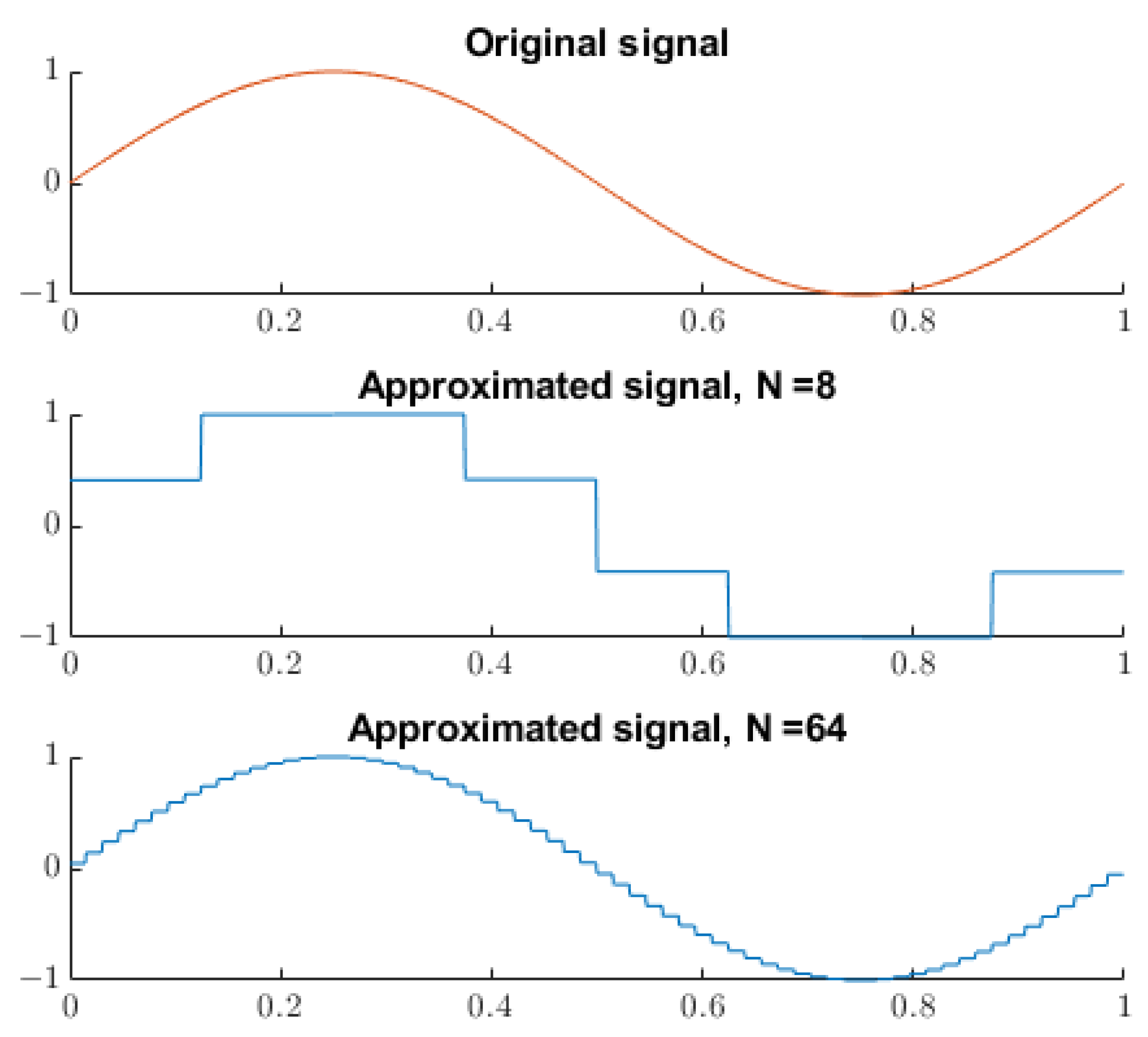
4. Signal Approximation—Orthogonal Expansion

The set of rows of matrix $A\left(n\right)$ defined by Equation (15) or Equation (4) represents the set of orthogonal discrete basis functions. We assume that these functions are defined within the interval $[0,T]$. In relation to the rows of matrix $A\left(n\right)$ we have:

$$\sum _{i,j}{\phi }_i·{\phi }_j=\left\{\begin{array}{c}0\mathrm{for}i\ne j\hfill \\ C\mathrm{for}i=j\hfill \end{array}\right.C=\sum _{i=1}^N{\left(a^i\right)}^2$$

(20)

An example of $N=4$ orthogonal basis functions based on matrix $A\left(2\right)$ for parameter $a=\frac{1}{2}$ is illustrated in Figure 1.

A continuous signal with finite energy $x\left(t\right)$ can be approximated by linear combinations of N orthogonal basis functions represented by rows of $A\left(n\right)$ [17]. Such an orthogonal expansion is expressed as follows:

$$x_A\left(t\right)=\sum _{i=1}^N{d}_i·{\phi }_i\left(t\right)$$

(21)

Multiplying both sides of the Equation (21) by ${\phi }_j\left(t\right)$, then integrating both sides and accounting for the orthogonality of the basis functions we obtain:

$$d_i=\frac{1}{C}\underset{0}{\overset{T}{\int }}{x}_A\left(t\right)·{\phi }_i\left(t\right)dt$$

(22)

where C is defined by Equation (20).

Figure 2 shows the approximated signals for a sinewave for the given N and selected value of a.

As can be seen from the results in Figure 1 (as expected), increasing the number of basis functions N decreases the value of the mean square error. For instance, for $N=4,8,32,64,128$ the $mse$ equals: $2.245\times {10}^{-1},3.09\times {10}^{-2},1.6\times {10}^{-3},$$4.0096\times {10}^{-4},$$9.8877\times {10}^{-5}$, respectively.

5. Proposed Orthogonal Transform and Its Modifications

5.1. One-Dimensional (1D) Transform

Let us consider a discrete one-dimensional signal represented by an N-element vector $X\left(n\right)=[x_1{x}_2\cdots x_N]$,$N=2^n$.

A 1D orthogonal Transform based on the matrix $A\left(n\right)$ defined earlier has the form:

$$\begin{array}{c}\hfill \begin{array}{cc}\hfill \mathrm{Forward}\mathrm{Transform}:S\left(n\right)& =A\left(n\right)·X\left(n\right)\hfill \\ \hfill \mathrm{Inverse}\mathrm{Transform}:X\left(n\right)& =\frac{1}{C}·A\left(n\right)·S\left(n\right)\hfill \end{array}\end{array}$$

(23)

where

• $S\left(n\right)$—vector of spectral components.
• $X\left(n\right)$—vector of 1D signal.
• $A\left(n\right)$—transform matrix defined by Equation (15).
• C—constant defined by Equation (16).

As was shown, the transform matrix $A\left(n\right)$ is symmetric and orthogonal and $A^T=A^{-1}$. Therefore, the forward transform (FT) differs from the inverse transform (IT) only by the constant C. Another more detailed form of the FT can be written as follows:

$$\begin{array}{c}\hfill \begin{array}{cc}\hfill \mathrm{FT}:\left[\begin{array}{c}{S}_1\\ S_2\\ ⋮\\ S_N\end{array}\right]& =\left[\begin{array}{cc}A(n-1)& A(n-1)·a^{2^{(n-1)}}\\ A(n-1)·a^{2^{(n-1)}}& -A(n-1)\end{array}\right]\left[\begin{array}{c}{x}_1\\ x_2\\ ⋮\\ x_N\end{array}\right]\hfill \\ \\ \hfill \mathrm{IT}:\left[\begin{array}{c}{x}_1\\ x_2\\ ⋮\\ x_N\end{array}\right]& =\frac{1}{C}·\left[\begin{array}{cc}A(n-1)& A(n-1)·a^{2^{(n-1)}}\\ A(n-1)·a^{2^{(n-1)}}& -A(n-1)\end{array}\right]\left[\begin{array}{c}{S}_1\\ S_2\\ ⋮\\ S_N\end{array}\right]\hfill \end{array}\end{array}$$

(24)

for $A\left(0\right)=a^k,k=1,2,3,\cdots$

We generally assume that $k=1$. Generally, we also assume that the parameter $a\ne 0$ is any real number within the interval $(-\infty ,+\infty )$. For a particular case $a=1$ the transform (24) becomes the 1D Walsh–Hadamard transform.

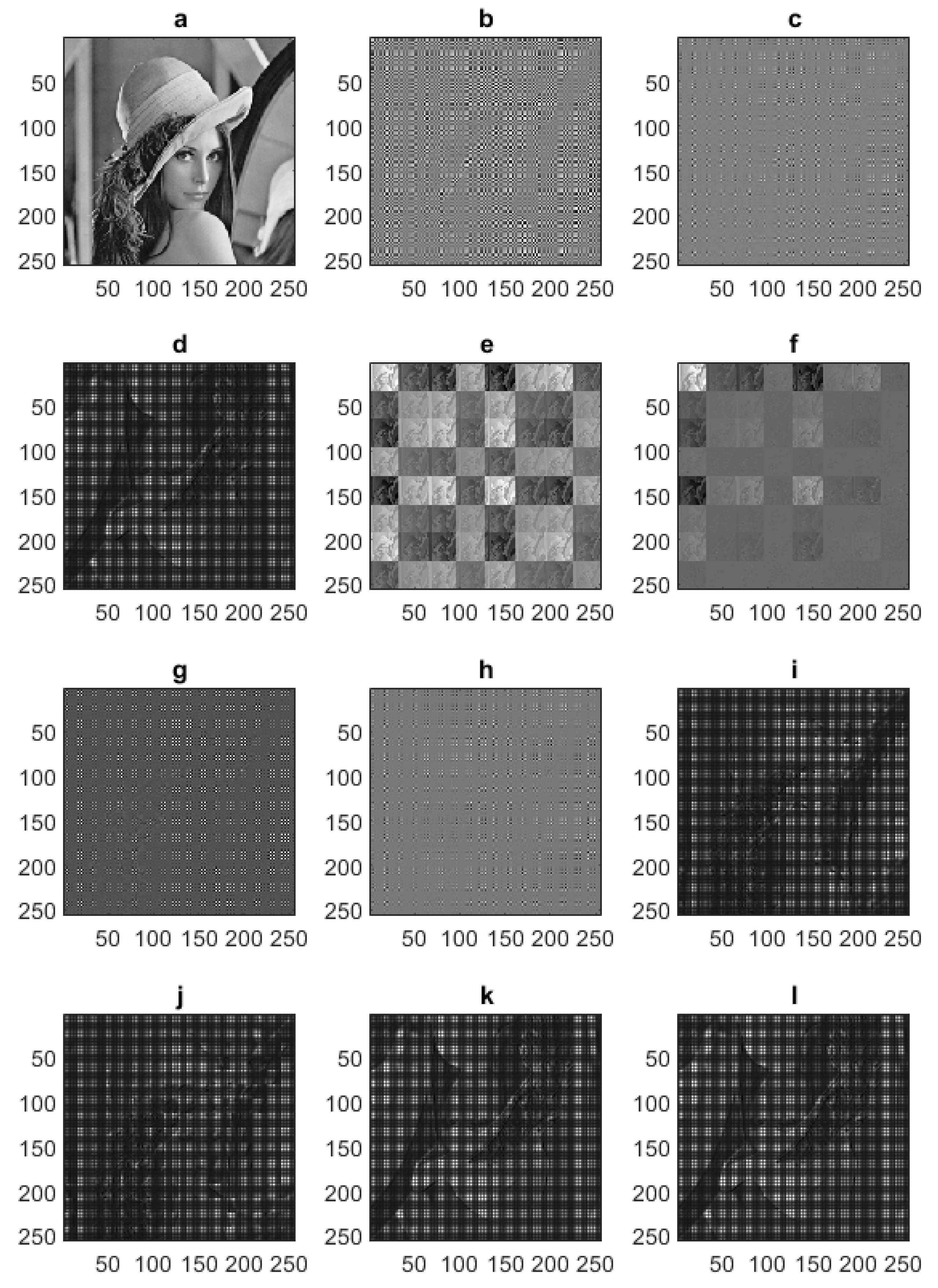
5.2. Two-Dimensional (2D) Transform

This case applies to two-dimensional signals represented by the square matrix $X(i,j)$ of N dimensions, $N=2^n,i=1,2,3,\dots ,N,j=1,2,3,\dots ,N$, which is mainly associated with image processing. In the general case a 2D transform has the form:

$$\begin{array}{c}\hfill \begin{array}{cc}\hfill \mathrm{FT}:S(i,j)& =A\left(n\right)·X(i,j)·A\left(n\right)\hfill \\ \hfill \mathrm{IT}:X(i,j)& =\frac{1}{C^2}·A\left(n\right)·S(i,j)·A\left(n\right)\hfill \end{array}\end{array}$$

(25)

where

• $S(i,j)$—matrix of spectral components.
• $X(i,j)$—matrix of 2D signal.
• $A\left(n\right)$—transform matrix described by Equation (15).
• C—constant described by Equation (16).

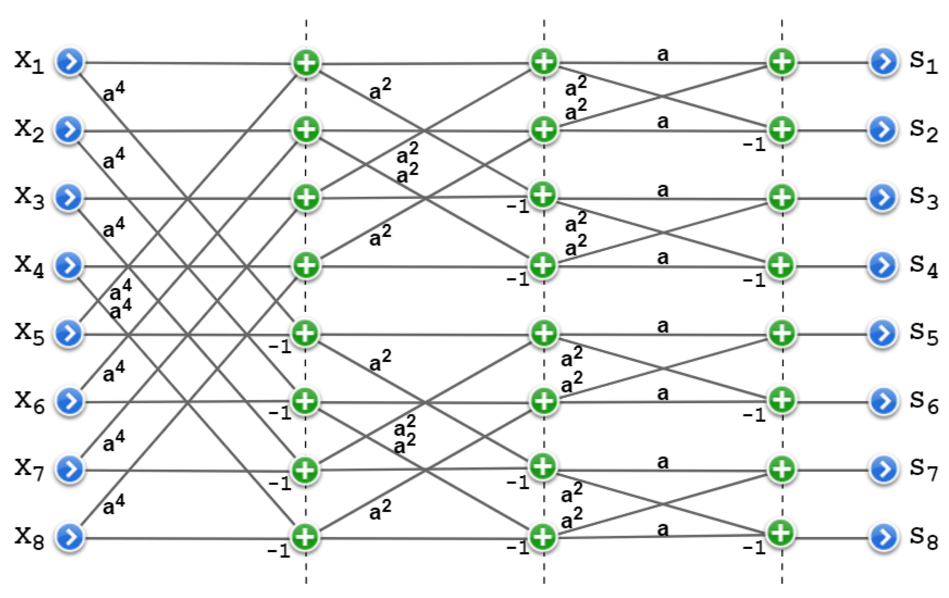
It is seen that the forward and inverse transforms have the same structure—they differ only in the constant C. The 2D transform can be calculated directly using Equation (24) or by grouping the channels as shown in Figure 3e,f. The transform matrix $A\left(n\right)$ consists of the power of parameter a. For $a=1$ we obtain the 2D Walsh–Hadamard transform. It is obvious that if the transform (25) is used for image processing we are dealing with large values of N. For this reason, large powers of parameter $a\ne 1$ may not be calculated by a computer. Thus, it seems purposeful to propose a sparse matrix $A_m\left(n\right)$ with the following form:

$$A_m\left(n\right)=\left[\begin{array}{ccccc}A\left(m\right)& 0& 0& \cdots & 0\\ 0& A\left(m\right)& 0& \cdots & 0\\ 0& 0& A\left(m\right)& \cdots & 0\\ ⋮& ⋮& ⋮& \ddots & ⋮\\ 0& 0& \hfill \cdots & & A\left(m\right)\end{array}\right]$$

(26a)

where $A_m\left(n\right)$—matrix with dimension $N=2^n,$$n=2,3,4,\dots$

$A\left(m\right)$—matrix (15) or (4) with dimension, $M=2^m,m=1,2,3,\dots ,m<n$.

For example, for the parameters $n=3$, $m=2$ the matrix $A_2\left(3\right)$ is:

$$A_2\left(3\right)=\left[\begin{array}{cc}A\left(2\right)& \cdots \\ \cdots & A\left(2\right)\end{array}\right]$$

(26b)

where $A\left(2\right)$ is defined either by (2) or (17b).

It is seen that like $A\left(n\right)$ matrix $A_m\left(n\right)$ is symmetric and orthogonal, so we have:

$$A_m\left(n\right)=A_m^T\left(n\right),A_m\left(n\right)·A_m^T\left(n\right)=C·I$$

(27)

$$A_m^{-1}\left(n\right)=A_m^T\left(n\right),I—\mathrm{unit}\mathrm{matrix}$$

$$\mathrm{where}C=\sum _{i=1}^{2^m}{a}^{2i}$$

(28)

The matrix $A_m\left(n\right)$ consists of many zeros, defined by:

$$L_0=N·(N-M)$$

(29)

The percentage ratio of the number of zeros to all elements of the matrix $A_m\left(n\right)$ is as follows:

$$\frac{L_0}{L_{total}}=\frac{N·(N-M)}{N^2}=(1-\frac{M}{N})·100\%$$

(30)

For instance, if $M=4,N=512$, more than 99% of the transform matrix $A_2\left(9\right)$ elements are zeros.

Matrix (26a) can therefore be used as a transform matrix for the following transform, which is a modified version of transforms (23) and (25) using submatrices $A\left(m\right)$.

$$\begin{array}{cc}& \hfill 1\mathrm{D}\mathrm{Transform}:\hfill \\ \mathrm{FT}:\hfill & S\left(n\right)=A_m\left(n\right)·X\left(n\right)\hfill \\ \mathrm{IT}:\hfill & X\left(n\right)=\frac{1}{C}·A_m\left(n\right)·S\left(n\right)\hfill \end{array}$$

(31)

$$\begin{array}{cc}& \hfill 2\mathrm{D}\mathrm{Transform}:\hfill \\ \mathrm{FT}:\hfill & S(i,j)=A_m\left(n\right)·X(i,j)·A_m\left(n\right)\hfill \\ \mathrm{IT}:\hfill & X(i,j)=\frac{1}{C^2}·A_m\left(n\right)·S(i,j)·A_m\left(n\right)\hfill \end{array}$$

(32)

$C$ is defined by Equation (28).

Transforms (31) and (32) with many zeros can be treated as a specific case of compression in the spatial domain. Calculating modified orthogonal transforms using sparse matrices expressed by (31) and (32) is not only simple but can also provide very fast calculations. However, this is the subject considered in the next section.

It is obvious that instead of using matrices (15) in all of the proposed orthogonal transforms (23), (25), (31) and (32) we can also use the symmetric and orthogonal matrix (4) as the transform matrix. In this case, we can consider different versions of the orthogonal transforms, in particular the transforms described by Equations (31) and (32) for which the submatrices $A\left(m\right)$ are the same or different. It was shown that each submatrix $A\left(m\right)$ of the matrix $A_m\left(n\right)$ is defined by the first three values of the basis sequence. For different submatrices we deal with a matrix of coefficients instead of coefficient C for the inverse transform.

Figure 3 shows: a—the input image for $N=256$ and its spectra obtained for various transform matrices; b—full exponential matrix ($N=256,a=0.3$); c—full exponential matrix ($N=256,a=0.7$); d—full non-exponential matrix ($N=256,$ basis sequence: $1,2,3$); e—full exponential matrix after channel grouping ($N=8,a=0.3;8\times 8$ channels); f—full exponential matrix after channel grouping ($N=8,a=0.7;8\times 8$ channels), g—sparse exponential matrix ($N=256,M=4,a=0.7$); h—sparse exponential matrix ($N=256,M=16,a=0.7$); i—sparse non-exponential matrix with the same submatrices ($N=256,M=8,$ basis sequence: $1,2,3$); j—sparse non-exponential matrix with the same submatrices ($N=256,M=16,$ basis sequence: $1,2,3$); k—full non-exponential matrix with arbitrary $\beta$ parameter ($N=256,\beta =0.75$ basis sequence: $1,2,3$); and l—full non-exponential matrix with arbitrary $\beta$ parameter ($N=256,\beta =1.25$ basis sequence: $1,2,3$).

In all cases after performing the inverse transforms we obtain the original input image.

6. Fast Algorithms

Fast algorithms are used to reduce the number of computations required to determine the transform coefficients in comparison to direct computation of the transform. The main idea of efficient or fast computational algorithms is the ability to subdivide the total computational load into a series of computational steps in such a way that partial results obtained from initial steps can be repeatedly utilized in the subsequent steps.

Fast computation of this matrix can be performed by the well-known techniques of sparse matrix factoring or matrix partitioning. These techniques result in fast algorithms that reduce the computation requirements from $N^2$ additions using direct computation to $N{log}_{2}N$ additions using fast algorithms [2].

In Figure 4, the flow graph of a fast algorithm for the computation of a full exponential orthogonal matrix for $N=8$ is presented.

The flow graph has a butterfly structure and is similar to the graph of the fast Walsh–Hadamard transform (WHT) algorithm [2].

The plot in Figure 5 shows the number of additions required for the proposed transform with respect to its dimensions. This plot also presents the comparison of the proposed transform (PT) and proposed sparse transforms (PST) for $M=4$ and $M=8$. with other well-known transforms, like periodic Haar piecewise-linear (PHL) [18], fast fourier (FFT), Walsh–Hadamard (WHT), Haar (HT), Slant (ST) and discrete cosine (DCT) transforms.

7. Conclusions

The method of creating symmetric, orthogonal matrices and orthogonal transforms presented in this paper is a generalization of Hadamard matrices and the Walsh–Hadamard transform. The experiments performed show that the proposed transforms can be effectively used for signal and image processing. The advantage of these transforms is simplicity of implementation and a relatively small number of operations necessary for calculations. Moreover, an important feature of the considered transforms is the possibility of forming spectral components of 1D and 2D signals by selecting the transform matrix parameters, in particular the parameter a. This feature, combined with the variety of structures of the considered orthogonal transforms, also offers promising possibilities for further applications.

References

1. Ahmed, N.; Rao, K.R. Orthogonal Transforms for Digital Signal Processing; Springer: Berlin/Heidelberg, Germany, 1975. [Google Scholar]
2. Wang, R. Introduction to Orthogonal Transforms: With Applications in Data Processing and Analysis; Cambridge University Press: Cambridge, UK, 2012. [Google Scholar]
3. Johnson, J.; Puschel, M. In search of the optimal Walsh–Hadamard transform. In Proceedings of the 2000 IEEE International Conference on Acoustics, Speech, and Signal Processing, Istanbul, Turkey, 5–9 June 2000; Volume 6, pp. 3347–3350. [Google Scholar]
4. Gonzalez, R.; Woods, R. Digital Image Processing, 4th ed.; Pearson: London, UK, 2018. [Google Scholar]
5. Madisetti, V. The Digital Signal Processing Handbook; CRC Press: Boca Raton, FL, USA, 2010. [Google Scholar]
6. Ashrafi, A. Chapter One—Walsh–Hadamard Transforms: A Review; Advances in Imaging and Electron Physics; Elsevier: Amsterdam, The Netherlands, 2017. [Google Scholar]
7. Sayood, K. Chapter 13—Transform Coding. Introduction to Data Compression, 5th ed.; The Morgan Kaufmann Series in Multimedia Information and Systems; Morgan Kaufmann: Burlington, MA, USA, 2018. [Google Scholar]
8. Hamood, M.; Boussakta, S. Fast Walsh–Hadamard–Fourier Transform Algorithm. IEEE Trans. Signal Process. 2011, 59, 5627–5631. [Google Scholar] [CrossRef]
9. Thompson, A. The Cascading Haar Wavelet Algorithm for Computing the Walsh–Hadamard Transform. IEEE Signal Process. Lett. 2017, 24, 1020–1023. [Google Scholar] [CrossRef] [Green Version]
10. Korus, P.; Dziech, A. Efficient Method for Content Reconstruction With Self-Embedding. IEEE Trans. Image Process. 2013, 22, 1134–1147. [Google Scholar] [CrossRef] [PubMed]
11. Korus, P.; Dziech, A. Adaptive Self-Embedding Scheme With Controlled Reconstruction Performance. IEEE Trans. Inf. Forensics Secur. 2014, 9, 169–181. [Google Scholar] [CrossRef]
12. Kalarikkal Pullayikodi, S.; Tarhuni, N.; Ahmed, A.; Shiginah, F.B. Computationally Efficient Robust Color Image Watermarking Using Fast Walsh Hadamard Transform. J. Imaging 2017, 3, 46. [Google Scholar] [CrossRef] [Green Version]
13. Pan, H.; Dabawi, D.; Cetin, A. Fast Walsh–Hadamard Transform and Smooth-Thresholding Based Binary Layers in Deep Neural Networks. In Proceedings of the IEEE/CVF Conference on Computer Vision and Pattern Recognition (CVPR) Workshops, Virtual Conference, 19–25 June 2021. [Google Scholar]
14. Subathra, M.S.P.; Mohammed, M.A.; Maashi, M.S.; Garcia-Zapirain, B.; Sairamya, N.J.; George, S.T. Detection of Focal and Non-Focal Electroencephalogram Signals Using Fast Walsh–Hadamard Transform and Artificial Neural Network. Sensors 2020, 20, 4952. [Google Scholar]
15. Wang, X.; Liang, X.; Zheng, J.; Zhou, H. Fast detection and segmentation of partial image blur based on discrete Walsh–Hadamard transform. Signal Process. Image Commun. 2019, 70, 47–56. [Google Scholar] [CrossRef]
16. Andrushia, A.D.; Thangarjan, R. Saliency-Based Image Compression Using Walsh–Hadamard Transform (WHT). In Biologically Rationalized Computing Techniques for Image Processing Applications; Springer: Cham, Switzerland, 2018. [Google Scholar]
17. Aristidi, E. Representation of Signals as Series of Orthogonal Functions. EAS Publ. Ser. 2016, 78–79, 99–126. [Google Scholar] [CrossRef] [Green Version]
18. Dziech, A.; Ślusarczyk, P.; Tibken, B. Methods of Image Compression by PHL Transform. J. Intell. Robot. Syst. 2004, 39, 447–458. [Google Scholar] [CrossRef]
Figure 1. Illustration of 4 orthogonal basis functions.
Applsci 11 07433 g001
Figure 2. Approximated signal for different N and a = 1 2 .
Applsci 11 07433 g002
Figure 3. Input image (a) and its spectra (bl) obtained for various transform matrices.
Applsci 11 07433 g003
Figure 4. Construction of fast algorithm for the computation of full exponential orthogonal matrix for N = 8 .
Applsci 11 07433 g004
Figure 5. Number of additions in relation to transform matrix size.
Applsci 11 07433 g005
Publisher’s Note: MDPI stays neutral with regard to jurisdictional claims in published maps and institutional affiliations.