
Evaluation of the Microsoft Excel Solver Spreadsheet-Based Program for Nonlinear Expressions of Adsorption Isotherm Models onto Magnetic Nanosorbent


 ,
,
Abstract
:1. Introduction
2. Materials and Methods
2.1. Isotherm Models
2.2. Error Function Analysis
2.3. Operational Software Tools
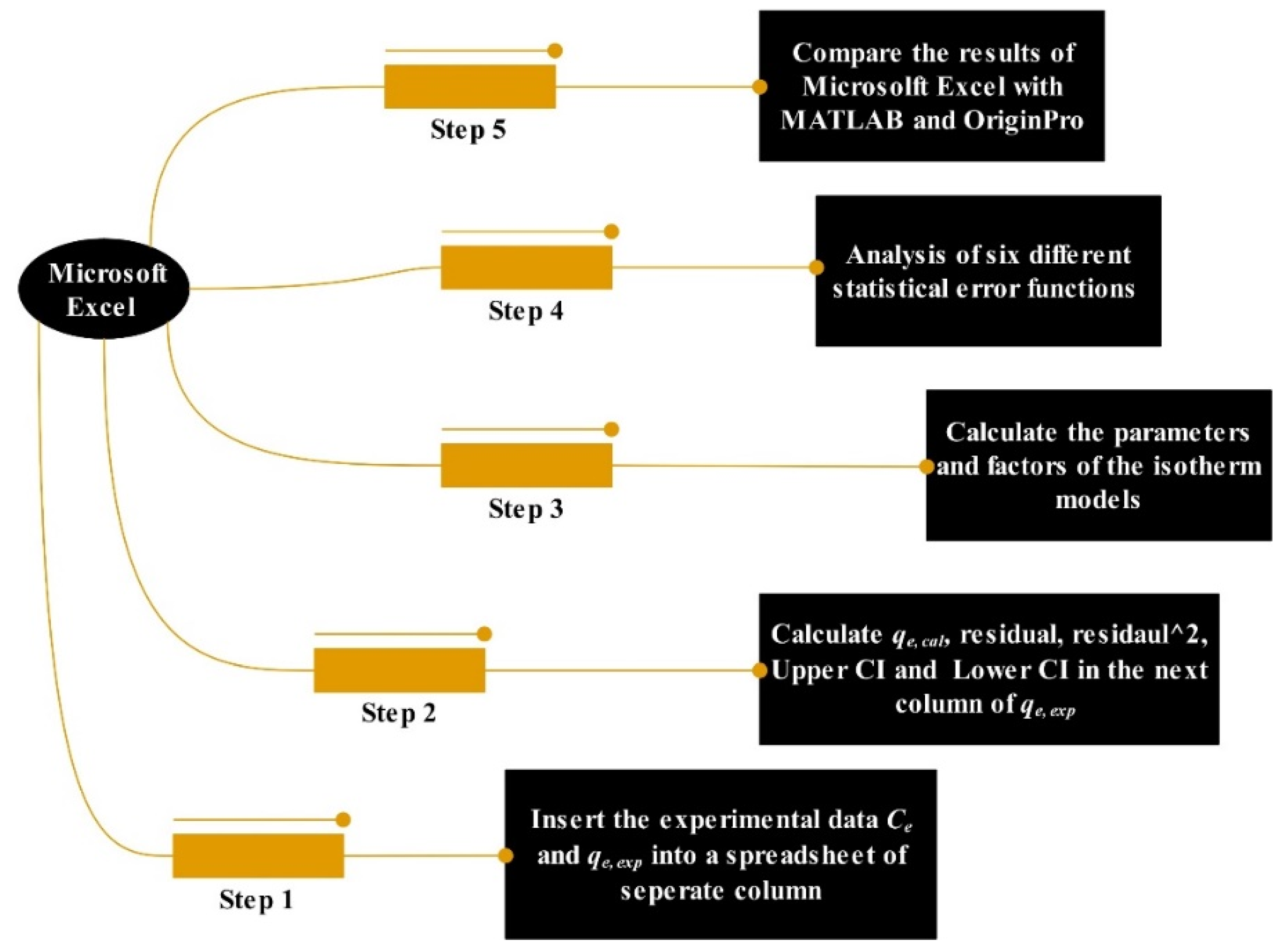
The Application of the Microsoft Excel Solver Spreadsheet Are as Follows
3. Results and Discussion
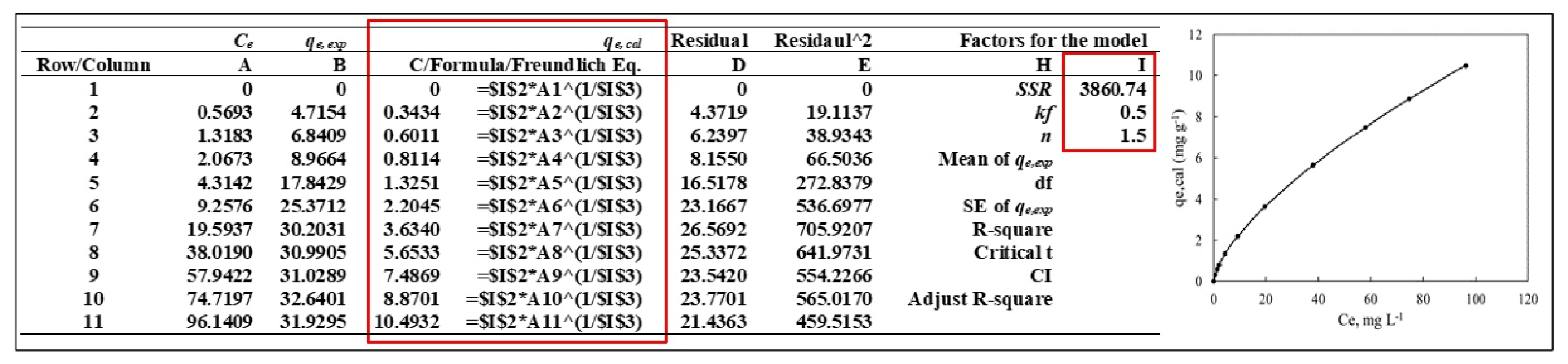
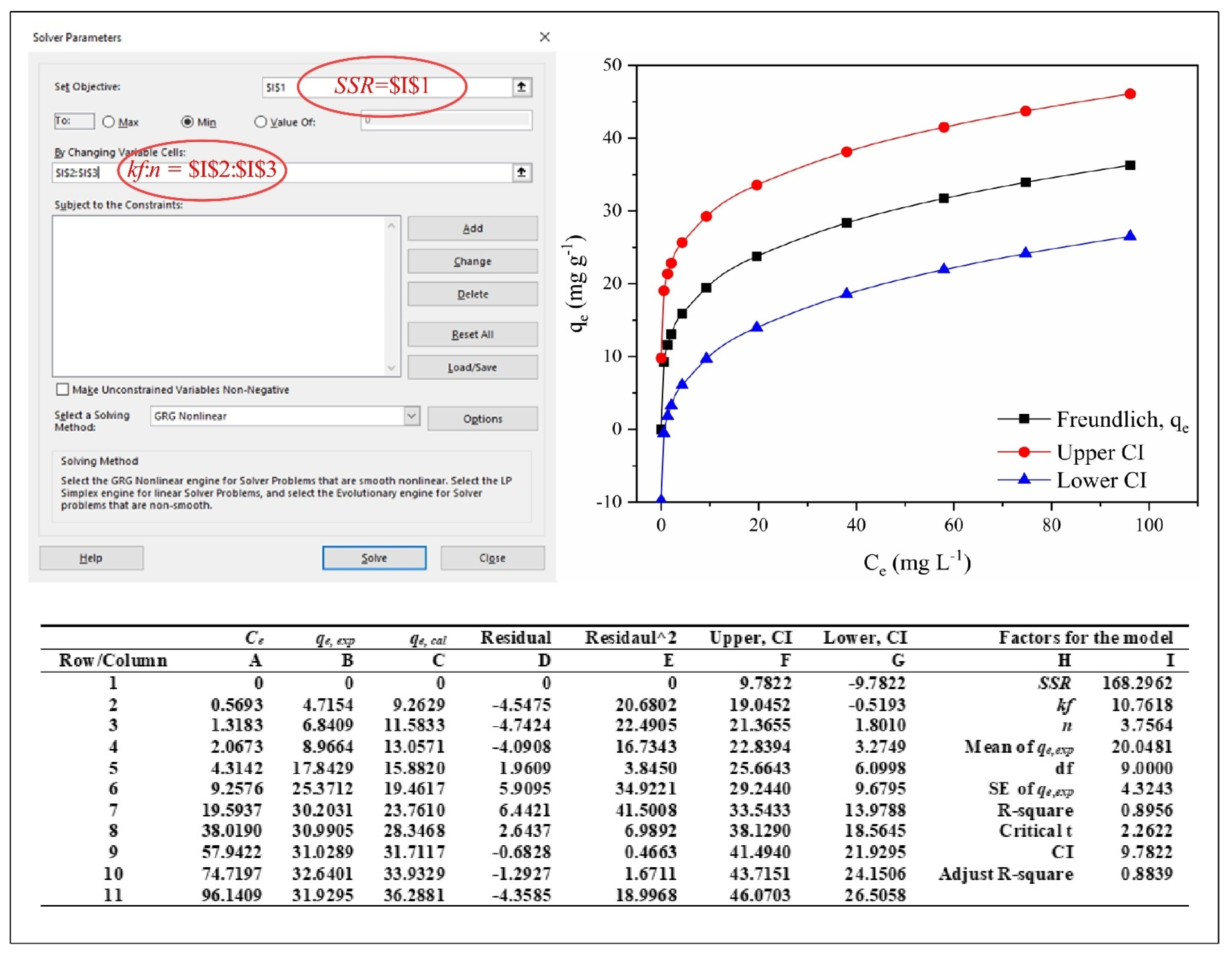
3.1. Authentication of Isotherm Model Data Using Microsoft Excel Solver Spreadsheet-Based Program
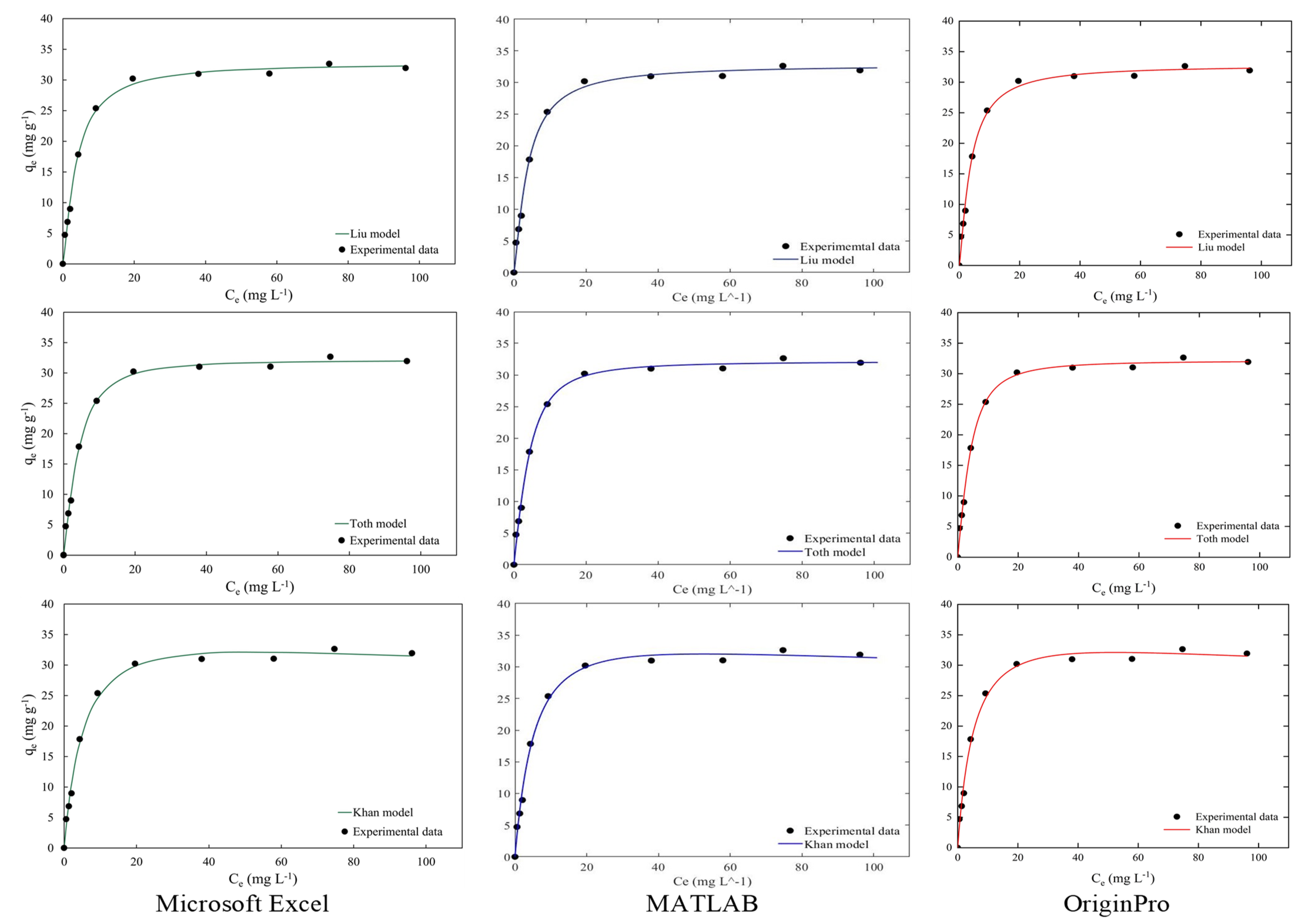
3.2. Comparison of Parameter Values for the Isotherm Models Obtained by Nonlinear Fitting
4. Conclusions
Author Contributions
Funding
Institutional Review Board Statement
Informed Consent Statement
Data Availability Statement
Acknowledgments
Conflicts of Interest
Nomenclature
| ak | Khan isotherm exponent (dimensionless) |
| bt | Temkin isotherm constant (J mol−1) |
| C0 | Initial concentration of adsorbate (mg L−1) |
| Ce | Concentration of adsorbate at equilibrium (mg L−1) |
| Ke | Thermodynamic equilibrium constant (dimensionless) |
| kf | Freundlich isotherm rate constant (mg g−1) (mg L−1)1/n |
| kg | Liu isotherm rate constant (L mg−1) |
| kk | Khan isotherm rate constant (L mg−1) |
| kl | Langmuir isotherm rate constant (L mg−1) |
| kr | Rate constant of general order model [h−1 (g mg−1)n−1] |
| kt | Temkin isotherm rate constant (L mol−1) |
| kth | Toth isotherm rate constant (L mg−1) |
| n | Order of reaction |
| nf | Heterogeneity factor (dimensionless) |
| ng | Liu isotherm exponent (dimensionless) |
| nth | Toth isotherm exponent (dimensionless) |
| qe | Predicted mass of MB adsorbed at equilibrium (mg g−1) |
| qex | Mass of MB adsorbed at equilibrium (experimental) (mg g−1) |
| qm | Maximum adsorption capacity (mg g−1) |
| R2 | Nonlinear coefficient of determination |
| SSE | Sum of squared error (residuals) |
| χ2 | Chi-square test |
Abbreviation
| ERRSQ/SSE | Residual Sum of Squares Error |
| ARE | Average Relative Error |
| HYBRID | Hybrid Fractional Error Function |
| MPSD | Marquardt’s Percent Standard Deviation |
| RMSE | Root Mean Square Error |
| MB | Methylene blue |
References
- Dias, J.M.; Alvim-Ferraz, M.C.M.; Almeida, M.F.; Rivera-Utrilla, J.; Sánchez-Polo, M. Waste materials for activated carbon preparation and its use in aqueous-phase treatment: A review. J. Environ. Manag. 2007, 85, 833–846. [Google Scholar] [CrossRef] [PubMed]
- Huang, Y.-P.; Hou, C.-H.; Hsi, H.-C.; Wu, J.-W. Optimization of highly microporous activated carbon preparation from Moso bamboo using central composite design approach. J. Taiwan Inst. Chem. Eng. 2015, 50, 266–275. [Google Scholar] [CrossRef]
- Shafeeyan, M.S.; Daud, W.M.A.W.; Houshmand, A.; Shamiri, A. A review on surface modification of activated carbon for carbon dioxide adsorption. J. Anal. Appl. Pyrolysis 2010, 89, 143–151. [Google Scholar] [CrossRef]
- Wickramaratne, N.P.; Jaroniec, M. Activated Carbon Spheres for CO2 Adsorption. ACS Appl. Mater. Interfaces 2013, 5, 1849–1855. [Google Scholar] [CrossRef]
- Zhou, L.; Wang, Y.; Liu, Z.; Huang, Q. Characteristics of equilibrium, kinetics studies for adsorption of Hg(II), Cu(II), and Ni(II) ions by thiourea-modified magnetic chitosan microspheres. J. Hazard. Mater. 2009, 161, 995–1002. [Google Scholar] [CrossRef]
- Oliveira, L.C.A.; Rios, R.V.R.A.; Fabris, J.D.; Sapag, K.; Garg, V.K.; Lago, R.M. Clay–iron oxide magnetic composites for the adsorption of contaminants in water. Appl. Clay Sci. 2003, 22, 169–177. [Google Scholar] [CrossRef]
- Yao, Y.; Miao, S.; Liu, S.; Ma, L.P.; Sun, H.; Wang, S. Synthesis, characterization, and adsorption properties of magnetic Fe3O4@graphene nanocomposite. Chem. Eng. J. 2012, 184, 326–332. [Google Scholar] [CrossRef]
- Ng, M.; Kho, E.T.; Liu, S.; Lim, M.; Amal, R. Highly adsorptive and regenerative magnetic TiO2 for natural organic matter (NOM) removal in water. Chem. Eng. J. 2014, 246, 196–203. [Google Scholar] [CrossRef]
- Bastami, T.R.; Entezari, M.H. Activated carbon from carrot dross combined with magnetite nanoparticles for the efficient removal of p-nitrophenol from aqueous solution. Chem. Eng. J. 2012, 210, 510–519. [Google Scholar] [CrossRef]
- Cheng, Z.; Gao, Z.; Ma, W.; Sun, Q.; Wang, B.; Wang, X. Preparation of magnetic Fe 3 O 4 particles modified sawdust as the adsorbent to remove strontium ions. Chem. Eng. J. 2012, 209, 451–457. [Google Scholar] [CrossRef]
- Wongcharee, S.; Aravinthan, V.; Erdei, L.; Sanongraj, W. Use of macadamia nut shell residues as magnetic nanosorbents. Int. Biodeterior. Biodegrad. 2017, 124, 276–287. [Google Scholar] [CrossRef]
- Bulut, Y.; Aydın, H. A kinetics and thermodynamics study of methylene blue adsorption on wheat shells. Desalination 2006, 194, 259–267. [Google Scholar] [CrossRef]
- Rida, K.; Bouraoui, S.; Hadnine, S. Adsorption of methylene blue from aqueous solution by kaolin and zeolite. Appl. Clay Sci. 2013, 83–84, 99–105. [Google Scholar] [CrossRef]
- Yagub, M.T.; Sen, T.K.; Ang, H.M. Equilibrium, Kinetics, and Thermodynamics of Methylene Blue Adsorption by Pine Tree Leaves. Water Air Soil Pollut. 2012, 223, 5267–5282. [Google Scholar] [CrossRef]
- Ayawei, N.; Jnr, M.H.; Spiff, I. Rhizophora mangle waste as adsorbent for metal ions removal from aqueous solution. Eur. J. Sci. Res. 2005, 9, 21. [Google Scholar]
- Shooto, N.; Ayawei, N.; Wankasi, D.; Sikhwivhilu, L.; Dikio, E. Study on cobalt metal organic framework material as adsorbent for lead ions removal in aqueous solution. Asian J. Chem. 2016, 28, 277. [Google Scholar] [CrossRef]
- Ahiduzzaman, M.; Islam, A.S. Preparation of porous bio-char and activated carbon from rice husk by leaching ash and chemical activation. SpringerPlus 2016, 5, 1248. [Google Scholar] [CrossRef] [Green Version]
- Wongcharee, S.; Aravinthan, V. Application of mesoporous magnetic nanosorbent developed from macadamia nut shell residues for the removal of recalcitrant melanoidin and its fractions. Sep. Sci. Technol. 2020, 55, 1636–1649. [Google Scholar] [CrossRef]
- Chincholi, M.; Sagwekar, P.; Nagaria, C.; Kulkarni, S.; Dhokpande, S. Removal of dye by adsorption on various adsorbents: A review. Int. J. Sci. Eng. Technol. Res. 2014, 3, 835–840. [Google Scholar]
- Edgar, T.F.; Himmelblau, D.M.; Lasdon, L.S. Optimization of Chemical Processes; McGraw-Hill: New York, NY, USA, 2001. [Google Scholar]
- Kumar, K.V.; Sivanesan, S. Pseudo second order kinetics and pseudo isotherms for malachite green onto activated carbon: Comparison of linear and non-linear regression methods. J. Hazard. Mater. 2006, 136, 721–726. [Google Scholar] [CrossRef] [PubMed]
- Pal, A. Statistical Analysis of Optimized Isotherm Model for Maxsorb III/Ethanol and Silica Gel/Water Pairs; School of Engineering Sciences, Kyushu University: Fukuoka, Japan, 2018. [Google Scholar]
- Jasper, E.E.; Ajibola, V.O.; Onwuka, J.C. Nonlinear regression analysis of the sorption of crystal violet and methylene blue from aqueous solutions onto an agro-waste derived activated carbon. Appl. Water Sci. 2020, 10, 132. [Google Scholar] [CrossRef]
- Kapoor, A.; Yang, R. Correlation of equilibrium adsorption data of condensible vapours on porous adsorbents. Gas Sep. Purif. 1989, 3, 187–192. [Google Scholar] [CrossRef]
- Foo, K.Y.; Hameed, B.H. Insights into the modeling of adsorption isotherm systems. Chem. Eng. J. 2010, 156, 2–10. [Google Scholar] [CrossRef]
- Chan, L.; Cheung, W.; Allen, S.; McKay, G. Error analysis of adsorption isotherm models for acid dyes onto bamboo derived activated carbon. Chin. J. Chem. Eng. 2012, 20, 535–542. [Google Scholar] [CrossRef]
- Azqhandi, M.H.A.; Foroughi, M.; Yazdankish, E. A highly effective, recyclable, and novel host-guest nanocomposite for Triclosan removal: A comprehensive modeling and optimization-based adsorption study. J. Colloid Interface Sci. 2019, 551, 195–207. [Google Scholar] [CrossRef]
- Bruce, P.; Bruce, A. Practical Statistics for Data Scientists: 50 Essential Concepts; O’Reilly Media: Newton, MA, USA, 2017. [Google Scholar]
- Shah, K.J.; Gandhi, V. Advances in Wastewater Treatment II; Materials Research Forum LLC: Millersville, PA, USA, 2021. [Google Scholar]
- Wongcharee, S.; Aravinthan, V.; Erdei, L.; Sanongraj, W. Mesoporous activated carbon prepared from macadamia nut shell waste by carbon dioxide activation: Comparative characterisation and study of methylene blue removal from aqueous solution. Asia Pac. J. Chem. Eng. 2018, 13, e2179. [Google Scholar] [CrossRef]
- Langmuir, I. The adsorption of gases on plane surfaces of glass, mica and platinum. J. Am. Chem. Soc. 1918, 40, 1361–1403. [Google Scholar] [CrossRef] [Green Version]
- Giles, C.H. The History and Use of the Freundlich Adsorption Isotherm. J. Soc. Dye. Colour. 1973, 89, 287–291. [Google Scholar] [CrossRef]
- Temkin, M. Kinetics of ammonia synthesis on promoted iron catalysts. Acta Physiochim. URSS 1940, 12, 327–356. [Google Scholar]
- Khan, A.; Ataullah, R.; Al-Haddad, A. Equilibrium adsorption studies of some aromatic pollutants from dilute aqueous solutions on activated carbon at different temperatures. J. Colloid Interface Sci. 1997, 194, 154–165. [Google Scholar] [CrossRef] [PubMed]
- Tóth, J. A uniform interpretation of gas/solid adsorption. J. Colloid Interface Sci. 1981, 79, 85–95. [Google Scholar] [CrossRef]
- Bergmann, C.P.; Machado, F.M. Carbon Nanomaterials as Adsorbents for Environmental and Biological Applications; Springer: Berlin/Heidelberg, Germany, 2015. [Google Scholar]
- Hossain, M.; Ngo, H.; Guo, W. Introductory of Microsoft Excel SOLVER function-spreadsheet method for isotherm and kinetics modelling of metals biosorption in water and wastewater. J. Water Sustain. 2013, 3, 223–237. [Google Scholar]
- Adekunbi, E.; Babajide, J.; Oloyede, H.; Amoko, J.; Obijole, O.; Oke, I. Evaluation of Microsoft excel solver as a tool for adsorption kinetics determination. IFE J. Sci. 2019, 21, 169–183. [Google Scholar] [CrossRef]
- Srenscek-Nazzal, J.; Narkiewicz, U.; Morawski, A.W.; Wrόbel, R.J.; Michalkiewicz, B. Comparison of optimized isotherm models and error functions for carbon dioxide adsorption on activated carbon. J. Chem. Eng. Data 2015, 60, 3148–3158. [Google Scholar] [CrossRef]
- Suwannahong, K.; Wongcharee, S.; Kreanuarte, J.; Kreetachart, T. Pre-treatment of acetic acid from food processing wastewater using response surface methodology via Fenton oxidation process for sustainable water reuse. J. Sustain. Dev. Energy Water Environ. Syst. 2020. [Google Scholar] [CrossRef]
- Puri, C.; Sumana, G. Highly effective adsorption of crystal violet dye from contaminated water using graphene oxide intercalated montmorillonite nanocomposite. Appl. Clay Sci. 2018, 166, 102–112. [Google Scholar] [CrossRef]
- Ayawei, N.; Ebelegi, A.N.; Wankasi, D. Modelling and Interpretation of Adsorption Isotherms. J. Chem. 2017, 2017, 3039817. [Google Scholar] [CrossRef]
- Vijayaraghavan, K.; Padmesh, T.; Palanivelu, K.; Velan, M. Biosorption of nickel (II) ions onto Sargassum wightii: Application of two-parameter and three-parameter isotherm models. J. Hazard. Mater. 2006, 133, 304–308. [Google Scholar] [CrossRef]
- Ho, Y.; Porter, J.; McKay, G. Equilibrium isotherm studies for the sorption of divalent metal ions onto peat: Copper, nickel and lead single component systems. Water Air Soil Pollut. 2002, 141, 1–33. [Google Scholar] [CrossRef]
- Liu, Y. Is the free energy change of adsorption correctly calculated? J. Chem. Eng. Data 2009, 54, 1981–1985. [Google Scholar] [CrossRef]
- Aufmann, R.N.; Lockwood, J. Mathematics: Journey from Basic Mathematics through Intermediate Algebra; Cengage Learning: Boston, MA, USA, 2020. [Google Scholar]
- Namakando, C. Zeropsis I; Fultus Corporation: Palo Alto, CA, USA, 2004. [Google Scholar]
- Huang, Y.-T.; Lee, L.-C.; Shih, M.-C.; Huang, W.-T. Introductory of Excel Spreadsheet for comparative analysis of linearized expressions of Langmuir isotherm for methylene blue onto rice husk. Int. J. Sci. Res. Publ. 2019, 9. [Google Scholar] [CrossRef]
- Bhatti, H.N.; Hayat, J.; Iqbal, M.; Noreen, S.; Nawaz, S. Biocomposite application for the phosphate ions removal in aqueous medium. J. Mater. Res. Technol. 2018, 7, 300–307. [Google Scholar] [CrossRef]


| Ce, Equilibrium Concentration (mg L−1) | qe,exp at Equilibrium (mg g−1) |
|---|---|
| 0 | 0 |
| 0.5693 | 4.7154 |
| 1.3183 | 6.8409 |
| 2.0673 | 8.9664 |
| 4.3142 | 17.8429 |
| 9.2576 | 25.3712 |
| 19.5937 | 30.2031 |
| 38.0190 | 30.9905 |
| 57.9422 | 31.0289 |
| 74.7197 | 32.6401 |
| 96.1409 | 31.9295 |
| Ce | qe, exp | qe, cal | Residual | Residaul^2 | Upper, CI | Lower, CI | Factors for the Model | Statistical Results | |||
|---|---|---|---|---|---|---|---|---|---|---|---|
| Row/Column | A | B | C | D | E | F | G | H | I | J | K |
| 1 | 0 | 0 | 0 | 0 | 0 | 9.7822 | −9.7822 | SSR | 168.2962 | ERRSQ/SSE | 168.2962 |
| 2 | 0.5693 | 4.7154 | 9.2629 | −4.5475 | 20.6802 | 19.0452 | −0.5193 | kf | 10.7618 | Chi-square | 13.3924 |
| 3 | 1.3183 | 6.8409 | 11.5833 | −4.7424 | 22.4905 | 21.3655 | 1.8010 | n | 3.7564 | ARE | −108.8583 |
| 4 | 2.0673 | 8.9664 | 13.0571 | −4.0908 | 16.7343 | 22.8394 | 3.2749 | Mean of qe,exp | 20.0481 | RMSE | 4.3243 |
| 5 | 4.3142 | 17.8429 | 15.8820 | 1.9609 | 3.8450 | 25.6643 | 6.0998 | df | 9.0000 | HYBRID | −20.8825 |
| 6 | 9.2576 | 25.3712 | 19.4617 | 5.9095 | 34.9221 | 29.2440 | 9.6795 | SE of qe,exp | 4.3243 | MPSD | 118.1294 |
| 7 | 19.5937 | 30.2031 | 23.7610 | 6.4421 | 41.5008 | 33.5433 | 13.9788 | R-square | 0.8956 | ||
| 8 | 38.0190 | 30.9905 | 28.3468 | 2.6437 | 6.9892 | 38.1290 | 18.5645 | Critical t | 2.2622 | ||
| 9 | 57.9422 | 31.0289 | 31.7117 | −0.6828 | 0.4663 | 41.4940 | 21.9295 | CI | 9.7822 | ||
| 10 | 74.7197 | 32.6401 | 33.9329 | −1.2927 | 1.6711 | 43.7151 | 24.1506 | Adjust R-square | 0.8839 | ||
| 11 | 96.1409 | 31.9295 | 36.2881 | −4.3585 | 18.9968 | 46.0703 | 26.5058 | ||||
| Formula or Excel code | |||||||||||
| qe, cal = $I$2 * A^(1/$I$3) Array Note: Values in column C (qe, cal) were depended on the values in column A (Ce), * = Multiplication sign (×). SSR = SUM(E1:E11) Array Mean of qe,exp = AVERAGE(B1:B11) Array df = COUNT(B1:B11)–COUNT(I2:I3) Array SE of qe,exp = SQRT(SUM((B1:B11–C1:C11)^2)/I6) Array R-square = 1-(SUM((B1:B11–C1:C11)^2)/(SUM((B1:B11-I5)^2))) Array Critical t = TINV(0.05,I6) Array CI = I7 * I9 Array Adjust R-square = (1–((COUNT(B1:B11)–1)/(COUNT(B1:B11)–2)) * (1–I8)) Array ERRSQ/SSE = SUM((C1:C11–B1:B11)^2) Array Chi-square = SUM(((C2:C11–B2:B11)^2)/(B2:B11)) Array ARE = (100 / (COUNT(B2:B11))) * (SUM((B2:B11–C2:C11)/(B2:B11))) Array RMSE = SQRT(SUM((B1:B11–C1:C11)^2)/(COUNT(C1:C11)–2)) Array HYBRID = (100/((COUNT(B2:B11))–(COUNT(I2:I3)))) * (SUM((B2:B11–C2:C11)/(B2:B11))) Array MPSD = 100 * SQRT((1/COUNT(B2:B11–I2:I3)*(SUM((B2:B11–C2:C11)/(B2:B11))^2))) Array | |||||||||||
| Ce | qe, exp | qe, cal | Residual | Residaul^2 | Upper, CI | Lower, CI | Factors for the Model | Statistical Results | |||
|---|---|---|---|---|---|---|---|---|---|---|---|
| Row/Column | A | B | C | D | E | F | G | H | I | J | K |
| 1 | 0 | 0 | 0 | 0 | 0 | 3.0777 | −3.0777 | SSR | 16.6590 | ERRSQ/SSE | 16.6590 |
| 2 | 0.5693 | 4.7154 | 4.0612 | 0.6541 | 0.4279 | 7.1389 | 0.9835 | kl | 0.2346 | Chi-square | 1.2540 |
| 3 | 1.3183 | 6.8409 | 8.1426 | −1.3018 | 1.6946 | 11.2203 | 5.0649 | qm | 34.4765 | ARE | −2.1538 |
| 4 | 2.0673 | 8.9664 | 11.2583 | −2.2919 | 5.2529 | 14.3360 | 8.1806 | Mean of qe,exp | 20.0481 | RMSE | 1.3605 |
| 5 | 4.3142 | 17.8429 | 17.3405 | 0.5024 | 0.2524 | 20.4182 | 14.2628 | df | 9.0000 | HYBRID | −2.3931 |
| 6 | 9.2576 | 25.3712 | 23.6056 | 1.7656 | 3.1174 | 26.6833 | 20.5279 | SE of qe,exp | 1.3605 | MPSD | 15.2297 |
| 7 | 19.5937 | 30.2031 | 28.3154 | 1.8877 | 3.5634 | 31.3931 | 25.2377 | R-square | 0.9897 | ||
| 8 | 38.0190 | 30.9905 | 31.0002 | −0.0097 | 0.0001 | 34.0779 | 27.9226 | Critical t | 2.2622 | ||
| 9 | 57.9422 | 31.0289 | 32.1136 | −1.0848 | 1.1767 | 35.1913 | 29.0359 | CI | 3.0777 | ||
| 10 | 74.7197 | 32.6401 | 32.6156 | 0.0246 | 0.0006 | 35.6933 | 29.5379 | Adjust R-square | 0.9885 | ||
| 11 | 96.1409 | 31.9295 | 33.0126 | −1.0831 | 1.1730 | 36.0903 | 29.9349 | ||||
| Formula or Excel code | |||||||||||
| qe, cal = ($I$3 * ($I$2 * (A/(1 + ($I$2 * A)))) Array Note: Values in column C (qe, cal) were depended on the values in column A (Ce), * = Multiplication sign (×). SSR = SUM(E1:E11) Array Mean of qe,exp = AVERAGE(B1:B11) Array df = COUNT(B1:B11)–COUNT(I2:I3) Array SE of qe,exp = SQRT(SUM((B1:B11–C1:C11)^2)/I6) Array R-square = 1-(SUM((B1:B11–C1:C11)^2)/(SUM((B1:B11-I5)^2))) Array Critical t = TINV(0.05,I6) Array CI = I7 * I9 Array Adjust R-square = (1–((COUNT(B1:B11)–1)/(COUNT(B1:B11)–2)) * (1–I8)) Array ERRSQ/SSE = SUM((C1:C11–B1:B11)^2) Array Chi-square = SUM(((C2:C11–B2:B11)^2)/(B2:B11)) Array ARE = (100/(COUNT(B2:B11))) * (SUM((B2:B11–C2:C11)/(B2:B11))) Array RMSE = SQRT(SUM((B1:B11–C1:C11)^2)/(COUNT(C1:C11)–2)) Array HYBRID = (100/((COUNT(B2:B11))–(COUNT(I2:I3)))) * (SUM((B2:B11–C2:C11)/(B2:B11))) Array MPSD = 100 * SQRT((1/COUNT(B2:B11–I2:I3) * (SUM((B2:B11–C2:C11) / (B2:B11))^2))) Array | |||||||||||
| Ce | qe, exp | qe, cal | Residual | Residaul^2 | Upper, CI | Lower, CI | Factors for the Model | Statistical Results | |||
|---|---|---|---|---|---|---|---|---|---|---|---|
| Row/Column | A | B | C | D | E | F | G | H | I | J | K |
| 1 | 0 | 0 | 0 | 0 | 0 | 6.9196 | −6.9196 | SSR | 72.0332 | ERRSQ/SSE | 72.0332 |
| 2 | 0.5693 | 4.7154 | 4.3210 | 0.3943 | 0.1555 | 11.2406 | −2.5986 | bt | 6.0492 | Chi-square | 4.0547 |
| 3 | 1.3183 | 6.8409 | 9.4006 | −2.5598 | 6.5524 | 16.3202 | 2.4810 | kt | 3.5884 | ARE | −4.0175 |
| 4 | 2.0673 | 8.9664 | 12.1222 | −3.1558 | 9.9593 | 19.0418 | 5.2026 | Mean of qe,exp | 20.0481 | RMSE | 2.8291 |
| 5 | 4.3142 | 17.8429 | 16.5726 | 1.2703 | 1.6137 | 23.4922 | 9.6530 | df | 8.0000 | HYBRID | −4.4639 |
| 6 | 9.2576 | 25.3712 | 21.1913 | 4.1799 | 17.4718 | 28.1109 | 14.2717 | SE of qe,exp | 3.0007 | MPSD | 28.4083 |
| 7 | 19.5937 | 30.2031 | 25.7267 | 4.4764 | 20.0382 | 32.6463 | 18.8071 | R-square | 0.9553 | ||
| 8 | 38.0190 | 30.9905 | 29.7366 | 1.2539 | 1.5723 | 36.6562 | 22.8170 | Critical t | 2.3060 | ||
| 9 | 57.9422 | 31.0289 | 32.2855 | −1.2566 | 1.5790 | 39.2051 | 25.3659 | CI | 6.9196 | ||
| 10 | 74.7197 | 32.6401 | 33.8238 | −1.1836 | 1.4010 | 40.7434 | 26.9042 | Adjust R-square | 0.9503 | ||
| 11 | 96.1409 | 31.9295 | 35.3486 | −3.4191 | 11.6900 | 42.2682 | 28.4290 | ||||
| Formula or Excel code | |||||||||||
| qe, cal = $I$2 * LN($I$3 * A) Array, Note: Values in column C (qe, cal) were depended on the values in column A (Ce), * = Multiplication sign (×). SSR = SUM(E1:E11) Array Mean of qe,exp = AVERAGE(B1:B11) Array df = COUNT(B1:B11)–COUNT(I2:I3) Array SE of qe,exp = SQRT(SUM((B1:B11–C1:C11)^2)/I6) Array R-square = 1-(SUM((B1:B11–C1:C11)^2)/(SUM((B1:B11-I5)^2))) Array Critical t = TINV(0.05,I6) Array CI = I7 * I9 Array Adjust R-square = (1–((COUNT(B1:B11)–1)/(COUNT(B1:B11)–2)) * (1–I8)) Array ERRSQ/SSE = SUM((C1:C11–B1:B11)^2) Array Chi-square = SUM(((C2:C11–B2:B11)^2)/(B2:B11)) Array ARE = (100/(COUNT(B2:B11))) * (SUM((B2:B11–C2:C11)/(B2:B11))) Array RMSE = SQRT(SUM((B1:B11–C1:C11)^2)/(COUNT(C1:C11)–2)) Array HYBRID = (100/((COUNT(B2:B11))–(COUNT(I2:I3)))) * (SUM((B2:B11–C2:C11)/(B2:B11))) Array MPSD = 100 * SQRT((1/COUNT(B2:B11–I2:I3) * (SUM((B2:B11–C2:C11)/(B2:B11))^2))) Array | |||||||||||
| Ce | qe, exp | qe, cal | Residual | Residaul^2 | Upper, CI | Lower, CI | Factors for the Model | Statistical Results | |||
|---|---|---|---|---|---|---|---|---|---|---|---|
| Row/Column | A | B | C | D | E | F | G | H | I | J | K |
| 1 | 0 | 0 | 0 | 0 | 0 | 2.3600 | −2.3600 | SSR | 8.3791 | ERRSQ/SSE | 8.3791 |
| 2 | 0.5693 | 4.7154 | 2.6272 | 2.0882 | 4.3606 | 4.9872 | 0.2672 | qm | 32.7792 | Chi-squar | 1.2093 |
| 3 | 1.3183 | 6.8409 | 6.7230 | 0.1179 | 0.0139 | 9.0830 | 4.3629 | kg | 0.2660 | ARE | 3.2148 |
| 4 | 2.0673 | 8.9664 | 10.3521 | −1.3858 | 1.9204 | 12.7122 | 7.9921 | ng | 0.7735 | RMSE | 1.0234 |
| 5 | 4.3142 | 17.8429 | 17.8449 | −0.0021 | 0.0000 | 20.2050 | 15.4849 | Mean of qe,exp | 20.0481 | HYBRID | 4.5926 |
| 6 | 9.2576 | 25.3712 | 24.9867 | 0.3845 | 0.1479 | 27.3467 | 22.6267 | df | 8.0000 | MPSD | 18.5609 |
| 7 | 19.5937 | 30.2031 | 29.3115 | 0.8916 | 0.7950 | 31.6715 | 26.9515 | SE of qe,exp | 1.0234 | ||
| 8 | 38.0190 | 30.9905 | 31.2120 | −0.2215 | 0.0490 | 33.5720 | 28.8520 | R-square | 0.9948 | ||
| 9 | 57.9422 | 31.0289 | 31.8516 | −0.8227 | 0.6769 | 34.2116 | 29.4916 | Critical t | 2.3060 | ||
| 10 | 74.7197 | 32.6401 | 32.1062 | 0.5340 | 0.2851 | 34.4662 | 29.7462 | CI | 2.3600 | ||
| 11 | 96.1409 | 31.9295 | 32.2906 | −0.3610 | 0.1304 | 34.6506 | 29.9306 | Adjust R-square | 0.9935 | ||
| Formula or Excel code | |||||||||||
| qe, cal = ($I$2 * ($I$3 * A)^(1/$I$4))/(1 + ($I$3 * A)^(1/$I$4)) Array, Note: Values in column C (qe, cal) were depended on the values in column A (Ce), * = Multiplication sign (×). SSR = SUM(E1:E11) Array Mean of qe,exp = AVERAGE(B1:B11) Array df = COUNT(B1:B11)–COUNT(I2:I3) Array SE of qe,exp = SQRT(SUM((B1:B11–C1:C11)^2)/I6) Array R-square = 1-(SUM((B1:B11–C1:C11)^2)/(SUM((B1:B11-I5)^2))) Array Critical t = TINV(0.05,I6) Array CI = I7 * I9 Array Adjust R-square = (1–((COUNT(B1:B11)–1)/(COUNT(B1:B11)–3)) * (1–I8)) Array ERRSQ/SSE = SUM((C1:C11–B1:B11)^2) Array Chi-square = SUM(((C2:C11–B2:B11)^2)/(B2:B11)) Array ARE = (100/(COUNT(B2:B11))) * (SUM((B2:B11–C2:C11)/(B2:B11))) Array RMSE = SQRT(SUM((B1:B11–C1:C11)^2)/(COUNT(C1:C11)–3)) Array HYBRID = (100/((COUNT(B2:B11))–(COUNT(I2:I4)))) * (SUM((B2:B11–C2:C11)/(B2:B11))) Array MPSD = 100 * SQRT((1/COUNT(B2:B11–I2:I4) * (SUM((B2:B11–C2:C11)/(B2:B11))^2))) Array | |||||||||||
| Ce | qe, exp | qe, cal | Residual | Residaul^2 | Upper, CI | Lower, CI | Factors for the Model | Statistical Results | |||
|---|---|---|---|---|---|---|---|---|---|---|---|
| Row/Column | A | B | C | D | E | F | G | H | I | J | K |
| 1 | 0 | 0 | 0 | 0 | 0 | 1.9260 | −1.9260 | SSR | 5.5806 | ERRSQ/SSE | 5.5806 |
| 2 | 0.5693 | 4.7154 | 2.9784 | 1.7369 | 3.0169 | 4.9044 | 1.0525 | qm | 32.1326 | Chi-squar | 0.8143 |
| 3 | 1.3183 | 6.8409 | 6.6830 | 0.1579 | 0.0249 | 8.6090 | 4.7570 | kth | 0.1645 | ARE | 2.8665 |
| 4 | 2.0673 | 8.9664 | 10.0211 | −1.0547 | 1.1124 | 11.9471 | 8.0951 | nth | 1.7045 | RMSE | 0.8325 |
| 5 | 4.3142 | 17.8429 | 17.5856 | 0.2573 | 0.0662 | 19.5116 | 15.6596 | Mean of qe,exp | 20.0481 | HYBRID | 4.0951 |
| 6 | 9.2576 | 25.3712 | 25.4476 | −0.0764 | 0.0058 | 27.3736 | 23.5216 | df | 8.0000 | MPSD | 16.5500 |
| 7 | 19.5937 | 30.2031 | 29.8163 | 0.3869 | 0.1497 | 31.7422 | 27.8903 | SE of qe,exp | 0.8352 | ||
| 8 | 38.0190 | 30.9905 | 31.3320 | −0.3415 | 0.1166 | 33.2580 | 29.4060 | R-square | 0.9965 | ||
| 9 | 57.9422 | 31.0289 | 31.7354 | −0.7065 | 0.4991 | 33.6614 | 29.8094 | Critical t | 2.3060 | ||
| 10 | 74.7197 | 32.6401 | 31.8736 | 0.7666 | 0.5877 | 33.7996 | 29.9476 | CI | 1.9260 | ||
| 11 | 96.1409 | 31.9295 | 31.9634 | −0.0338 | 0.0011 | 33.8894 | 30.0374 | Adjust R-square | 0.9957 | ||
| Formula or Excel code | |||||||||||
| qe, cal = $I$2 * (($I$3 * A)/((1 + ($I$3 * A)^($I$4))^(1/$I$4))) Array, Note: Values in column C (qe, cal) were depended on the values in column A (Ce), * = Multiplication sign (×). SSR = SUM(E1:E11) Array Mean of qe,exp = AVERAGE(B1:B11) Array df = COUNT(B1:B11)–COUNT(I2:I3) Array SE of qe,exp = SQRT(SUM((B1:B11–C1:C11)^2)/I6) Array R-square = 1-(SUM((B1:B11–C1:C11)^2)/(SUM((B1:B11-I5)^2))) Array Critical t = TINV(0.05,I6) Array CI = I7 * I9 Array Adjust R-square = (1–((COUNT(B1:B11)–1)/(COUNT(B1:B11)–3)) * (1–I8)) Array ERRSQ/SSE = SUM((C1:C11–B1:B11)^2) Array Chi-square = SUM(((C2:C11–B2:B11)^2)/(B2:B11)) Array ARE = (100/(COUNT(B2:B11))) * (SUM((B2:B11–C2:C11)/(B2:B11))) Array RMSE = SQRT(SUM((B1:B11–C1:C11)^2)/(COUNT(C1:C11)–3)) Array HYBRID = (100/((COUNT(B2:B11))–(COUNT(I2:I4)))) * (SUM((B2:B11–C2:C11)/(B2:B11))) Array MPSD = 100 * SQRT((1/COUNT(B2:B11–I2:I4) * (SUM((B2:B11–C2:C11)/(B2:B11))^2))) Array | |||||||||||
| Ce | qe, exp | qe, cal | Residual | Residaul^2 | Upper, CI | Lower, CI | Factors for the Model | Statistical Results | |||
|---|---|---|---|---|---|---|---|---|---|---|---|
| Row/Column | A | B | C | D | E | F | G | H | I | J | K |
| 1 | 0 | 0 | 0 | 0 | 0 | 2.3249 | −2.3249 | SSR | 8.1318 | ERRSQ/SSE | 8.1318 |
| 2 | 0.5693 | 4.7154 | 3.5660 | 1.1494 | 1.3211 | 5.8909 | 1.2410 | qm | 48.6815 | Chi-squar | 0.7585 |
| 3 | 1.3183 | 6.8409 | 7.4303 | −0.5894 | 0.3474 | 9.7552 | 5.1054 | kk | 0.1404 | ARE | 0.3101 |
| 4 | 2.0673 | 8.9664 | 10.5790 | −1.6126 | 2.6006 | 12.9039 | 8.2541 | ak | 1.1361 | RMSE | 1.0082 |
| 5 | 4.3142 | 17.8429 | 17.2192 | 0.6237 | 0.3890 | 19.5441 | 14.8943 | Mean of qe,exp | 20.0481 | HYBRID | 0.4430 |
| 6 | 9.2576 | 25.3712 | 24.5664 | 0.8048 | 0.6477 | 26.8913 | 22.2415 | df | 8.0000 | MPSD | 1.7904 |
| 7 | 19.5937 | 30.2031 | 29.8242 | 0.3789 | 0.1436 | 32.1492 | 27.4993 | SE of qe,exp | 1.0082 | ||
| 8 | 38.0190 | 30.9905 | 31.8887 | −0.8982 | 0.8067 | 34.2136 | 29.5638 | R-square | 0.9950 | ||
| 9 | 57.9422 | 31.0289 | 32.0809 | −1.0520 | 1.1068 | 34.4058 | 29.7560 | Critical t | 2.3060 | ||
| 10 | 74.7197 | 32.6401 | 31.8781 | 0.7621 | 0.5808 | 34.2030 | 29.5531 | CI | 2.3249 | ||
| 11 | 96.1409 | 31.9295 | 31.4957 | 0.4338 | 0.1882 | 33.8206 | 29.1708 | Adjust R-square | 0.9937 | ||
| Formula or Excel code | |||||||||||
| qe, cal = ($I$2 * $I$3 * A)/((1 + ($I$3 * A))^$I$4) Array, Note: Values in column C (qe, cal) were depended on the values in column A (Ce), * = Multiplication sign (×). SSR = SUM(E1:E11) Array Mean of qe,exp = AVERAGE(B1:B11) Array df = COUNT(B1:B11)–COUNT(I2:I3) Array SE of qe,exp = SQRT(SUM((B1:B11–C1:C11)^2)/I6) Array R-square = 1-(SUM((B1:B11–C1:C11)^2)/(SUM((B1:B11-I5)^2))) Array Critical t = TINV(0.05,I6) Array CI = I7 * I9 Array Adjust R-square = (1–((COUNT(B1:B11)–1)/(COUNT(B1:B11)–3)) * (1–I8)) Array ERRSQ/SSE = SUM((C1:C11–B1:B11)^2) Array Chi-square = SUM(((C2:C11–B2:B11)^2)/(B2:B11)) Array ARE = (100/(COUNT(B2:B11))) * (SUM((B2:B11–C2:C11)/(B2:B11))) Array RMSE = SQRT(SUM((B1:B11–C1:C11)^2)/(COUNT(C1:C11)–3)) Array HYBRID = (100/((COUNT(B2:B11))–(COUNT(I2:I4)))) * (SUM((B2:B11–C2:C11)/(B2:B11))) Array MPSD = 100 * SQRT((1/COUNT(B2:B11–I2:I4) * (SUM((B2:B11–C2:C11)/(B2:B11))^2))) Array | |||||||||||
| Model Parameter | Equation | Parameter Values for the Isotherm Models | ||
|---|---|---|---|---|
| Microsoft Excel Solver Functions | MATLAB | OriginPro | ||
| Freundlich | ||||
| kf | 10.76 | 10.76 | 10.76 | |
| nf | 3.7564 | 3.757 | 3.756 | |
| 1/nf | 0.2662 | 0.2662 | 2.2662 | |
| R-square | 0.8955 | 0.8955 | 0.8955 | |
| Adj R-square | 0.8839 | 0.8839 | 0.8839 | |
| ERRSQ/SSE | 168.2962 | 168.2962 | 168.2963 | |
| Chi-square | 13.39 | - | 13.39 | |
| ARE | −16.71 | - | - | |
| RMSE | 4.3243 | 4.3243 | - | |
| HYBRID | −20.88 | - | - | |
| MPSD | 118.1294 | - | - | |
| Langmuir | ||||
| qm | 34.48 | 34.48 | 34.48 | |
| kl | 0.2346 | 0.2343 | 0.2346 | |
| R-square | 0.9897 | 0.9897 | 0.9897 | |
| Adj R-square | 0.9885 | 0.9885 | 0.9885 | |
| ERRSQ/SSE | 16.6590 | 16.6590 | 16.6590 | |
| Chi-square | 1.254 | - | 1.254 | |
| ARE | −2.154 | - | - | |
| RMSE | 1.3605 | 1.3605 | - | |
| HYBRID | −2.393 | - | - | |
| MPSD | 15.2297 | - | - | |
| Temkin | ||||
| bt | 6.049 | 6.049 | 6.049 | |
| kt | 3.588 | 3.588 | 3.588 | |
| R-square | 0.9553 | 0.9384 | 0.9553 | |
| Adj R-square | 0.9503 | 0.9306 | 0.9503 | |
| ERRSQ/SSE | 72.0332 | 72.0332 | 72.0332 | |
| Chi-square | 4.055 | - | 4.055 | |
| ARE | −4.018 | - | - | |
| RMSE | 2.8291 | 3.0001 | - | |
| HYBRID | −4.464 | - | - | |
| MPSD | 28.4083 | - | - | |
| Liu [45] | ||||
| qm | 32.78 | 32.78 | 32.78 | |
| kg | 0.2660 | 0.2660 | 0.2660 | |
| ng | 0.7735 | 0.7735 | 1.2928 | |
| R-square | 0.9948 | 0.9948 | 0.9948 | |
| Adj R-square | 0.9935 | 0.9935 | 0.9935 | |
| ERRSQ/SSE | 8.3791 | 8.3791 | 8.3791 | |
| Chi-square | 1.209 | - | 1.209 | |
| ARE | 3.215 | - | - | |
| RMSE | 1.0234 | 1.0234 | - | |
| HYBRID | 4.593 | - | - | |
| MPSD | 18.5609 | - | - | |
| Toth [35] | ||||
| qm | 32.13 | 32.13 | 32.13 | |
| kth | 0.1645 | 0.1645 | 0.1645 | |
| nth | 1.705 | 1.705 | 1.705 | |
| R-square | 0.9965 | 0.9965 | 0.9965 | |
| Adj R-square | 0.9957 | 0.9957 | 0.9957 | |
| ERRSQ/SSE | 5.5806 | 5.5806 | 5.5086 | |
| Chi-square | 0.814 | - | 0.814 | |
| ARE | 2.867 | - | - | |
| RMSE | 0.8352 | 0.8352 | - | |
| HYBRID | 4.095 | - | - | |
| MPSD | 16.5500 | - | - | |
| Khan | ||||
| qm | 48.68 | 43.84 | 48.71 | |
| kk | 0.1404 | 0.1462 | 0.1403 | |
| ak | 1.136 | 1.105 | 1.136 | |
| R-square | 0.9950 | 0.9954 | 0.9950 | |
| Adj R-square | 0.9937 | 0.9943 | 0.9937 | |
| ERRSQ/SSE | 8.1318 | 7.3538 | 8.1318 | |
| Chi-squar | 0.7585 | - | 0.7585 | |
| ARE | 0.310 | - | - | |
| RMSE | 1.0082 | 0.9588 | - | |
| HYBRID | 0.4430 | - | - | |
| MPSD | 1.7904 | - | - | |
Publisher’s Note: MDPI stays neutral with regard to jurisdictional claims in published maps and institutional affiliations. |
© 2021 by the authors. Licensee MDPI, Basel, Switzerland. This article is an open access article distributed under the terms and conditions of the Creative Commons Attribution (CC BY) license (https://creativecommons.org/licenses/by/4.0/).
Share and Cite
Suwannahong, K.; Wongcharee, S.; Kreetachart, T.; Sirilamduan, C.; Rioyo, J.; Wongphat, A. Evaluation of the Microsoft Excel Solver Spreadsheet-Based Program for Nonlinear Expressions of Adsorption Isotherm Models onto Magnetic Nanosorbent. Appl. Sci. 2021, 11, 7432. https://doi.org/10.3390/app11167432
Suwannahong K, Wongcharee S, Kreetachart T, Sirilamduan C, Rioyo J, Wongphat A. Evaluation of the Microsoft Excel Solver Spreadsheet-Based Program for Nonlinear Expressions of Adsorption Isotherm Models onto Magnetic Nanosorbent. Applied Sciences. 2021; 11(16):7432. https://doi.org/10.3390/app11167432
Chicago/Turabian StyleSuwannahong, Kowit, Surachai Wongcharee, Torpong Kreetachart, Chadrudee Sirilamduan, Javier Rioyo, and Akkharaphong Wongphat. 2021. "Evaluation of the Microsoft Excel Solver Spreadsheet-Based Program for Nonlinear Expressions of Adsorption Isotherm Models onto Magnetic Nanosorbent" Applied Sciences 11, no. 16: 7432. https://doi.org/10.3390/app11167432
APA StyleSuwannahong, K., Wongcharee, S., Kreetachart, T., Sirilamduan, C., Rioyo, J., & Wongphat, A. (2021). Evaluation of the Microsoft Excel Solver Spreadsheet-Based Program for Nonlinear Expressions of Adsorption Isotherm Models onto Magnetic Nanosorbent. Applied Sciences, 11(16), 7432. https://doi.org/10.3390/app11167432