
Assessing and Modelling the Interactions of Instrumented Particles with Bed Surface at Low Transport Conditions


Abstract
:Featured Application
Abstract
1. Introduction
1.1. Background to Bed Load Transport Processes
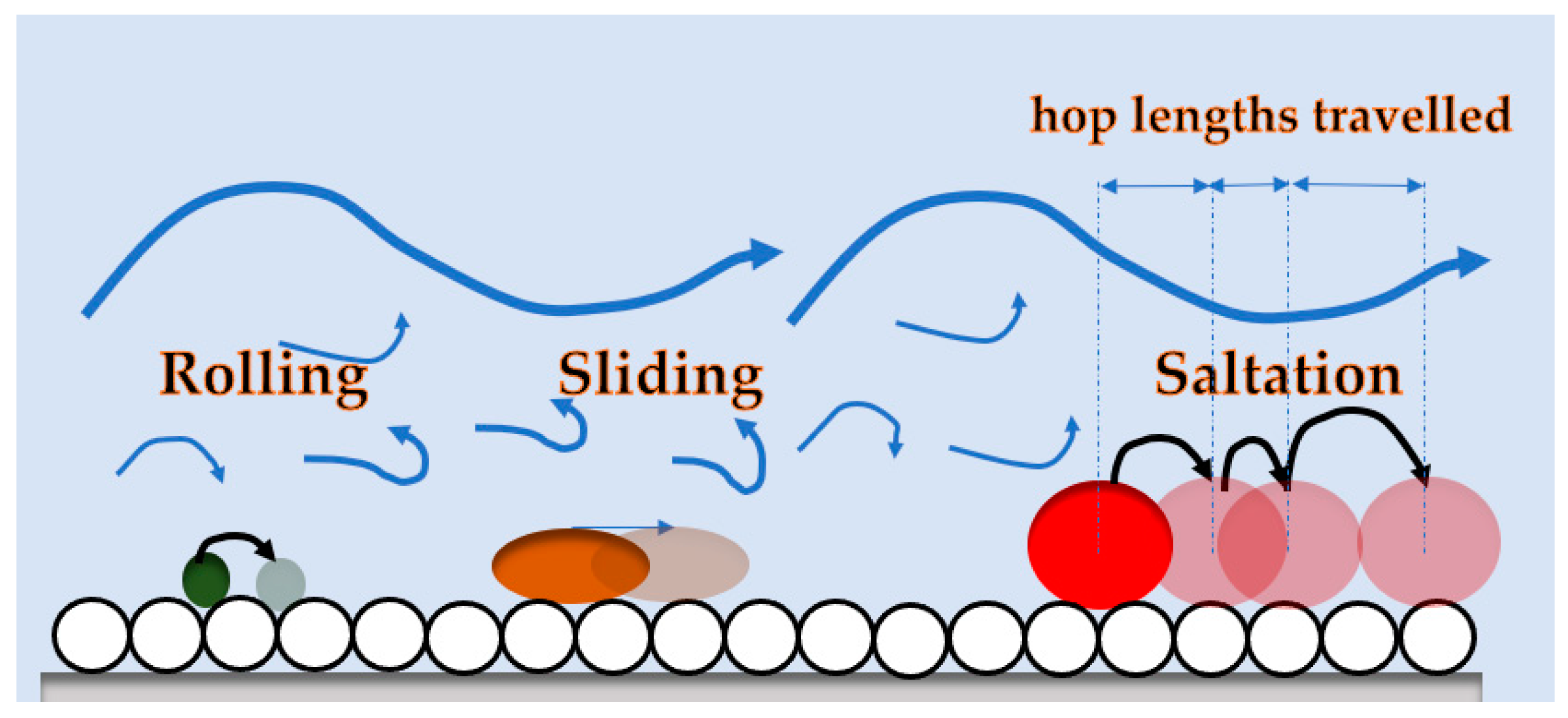
1.2. Conceptual Description of Transport Processes by Hopping
1.3. Lagrangian Observations of Transport Processes Facilitated via Novel Sensing Tools
1.4. Outlook for the Current Study
2. Experimental Methodology
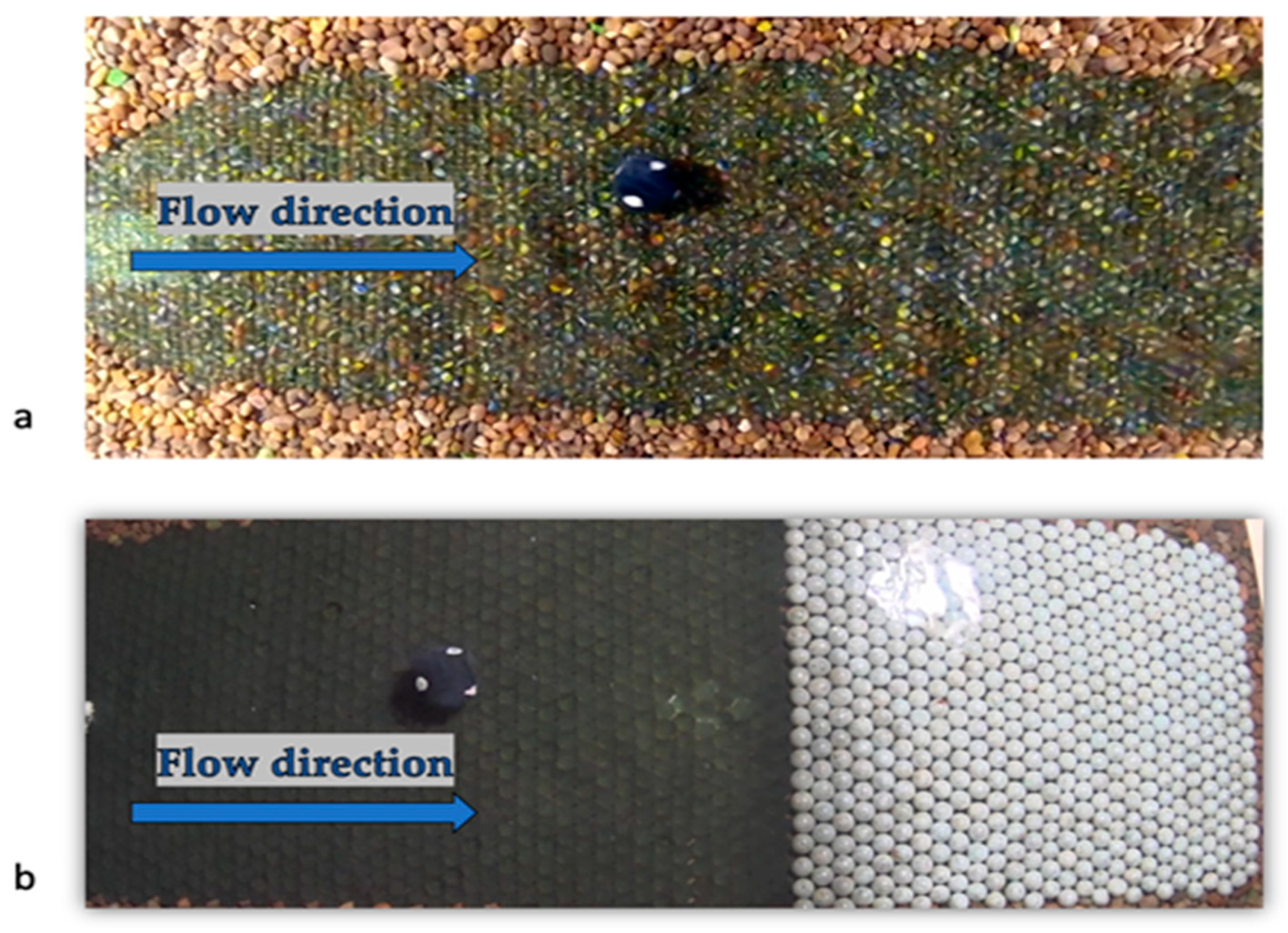
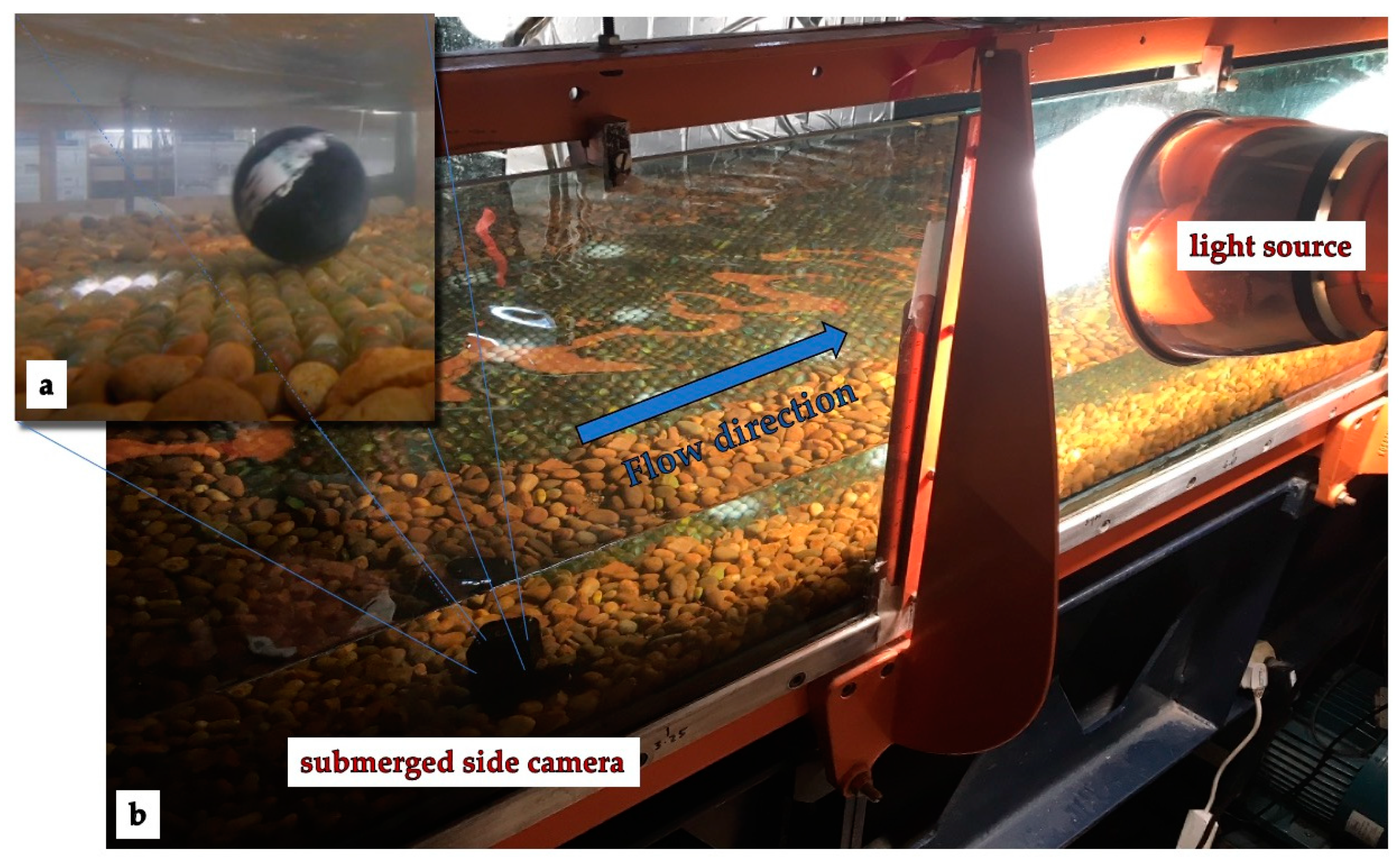
2.1. Experimental Set Up
2.2. Experimental Equipment and Instrumentation
2.2.1. Flow Velocimetry
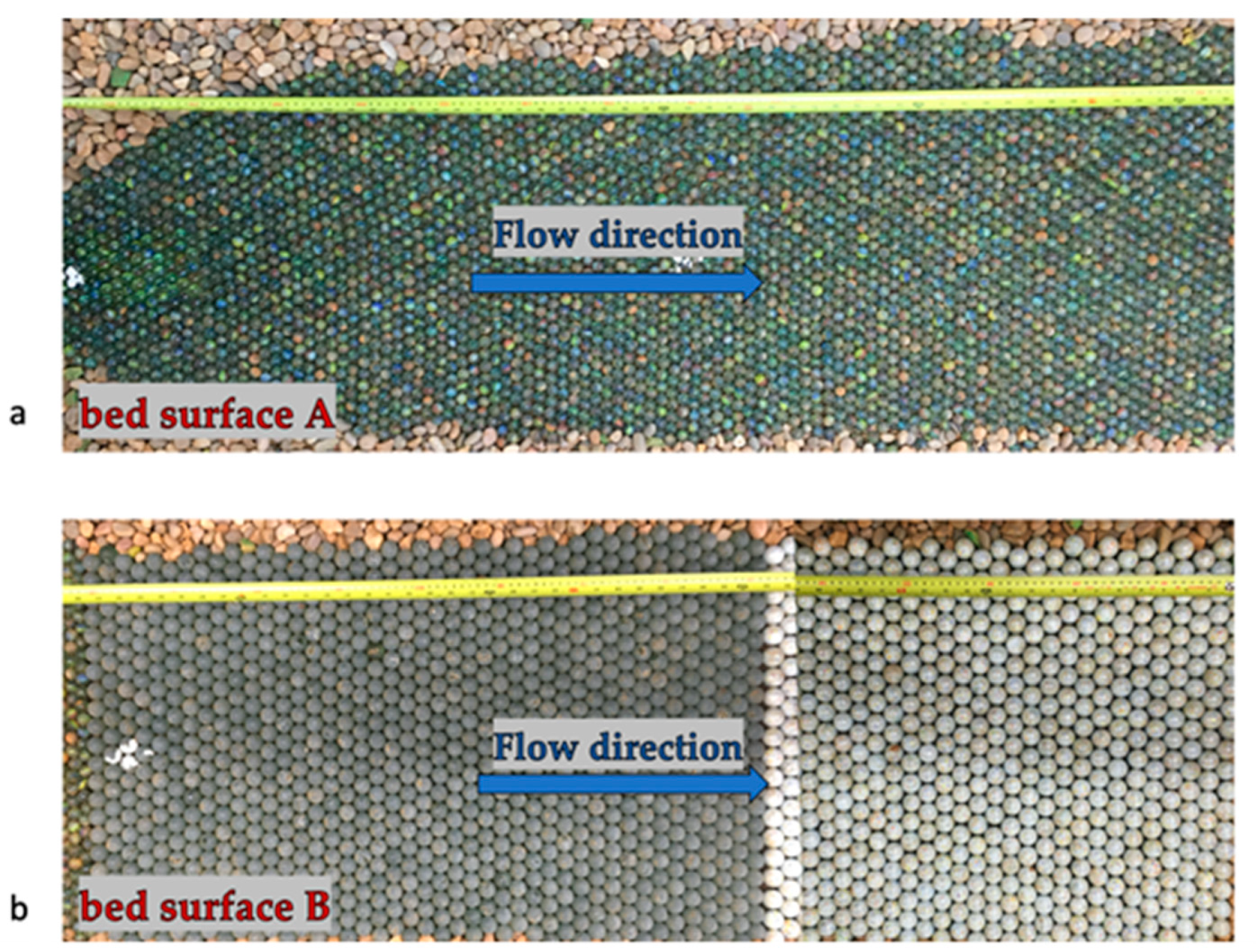
2.2.2. Particle Transport Tracking: Visual Methods
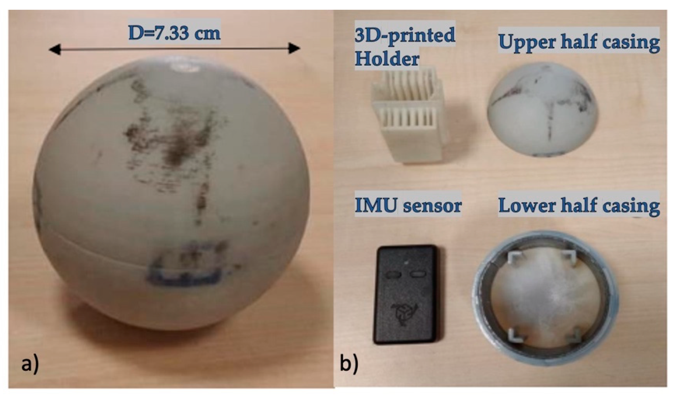
2.2.3. Particle Transport Tracking: IMU Embedded Instrumented Particle
2.3. Experimental Matrix and Protocol
3. Results
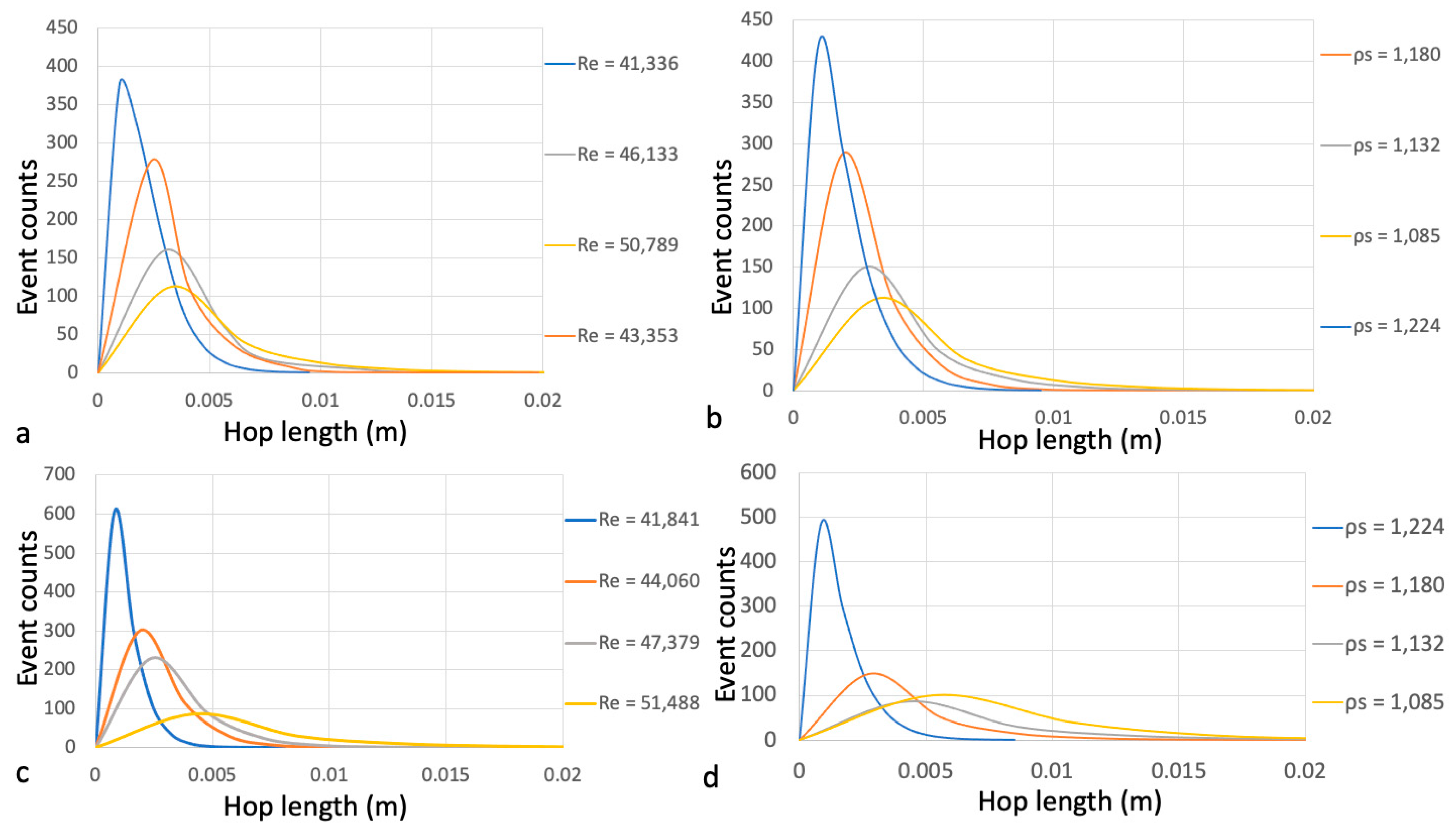
3.1. Hop Length
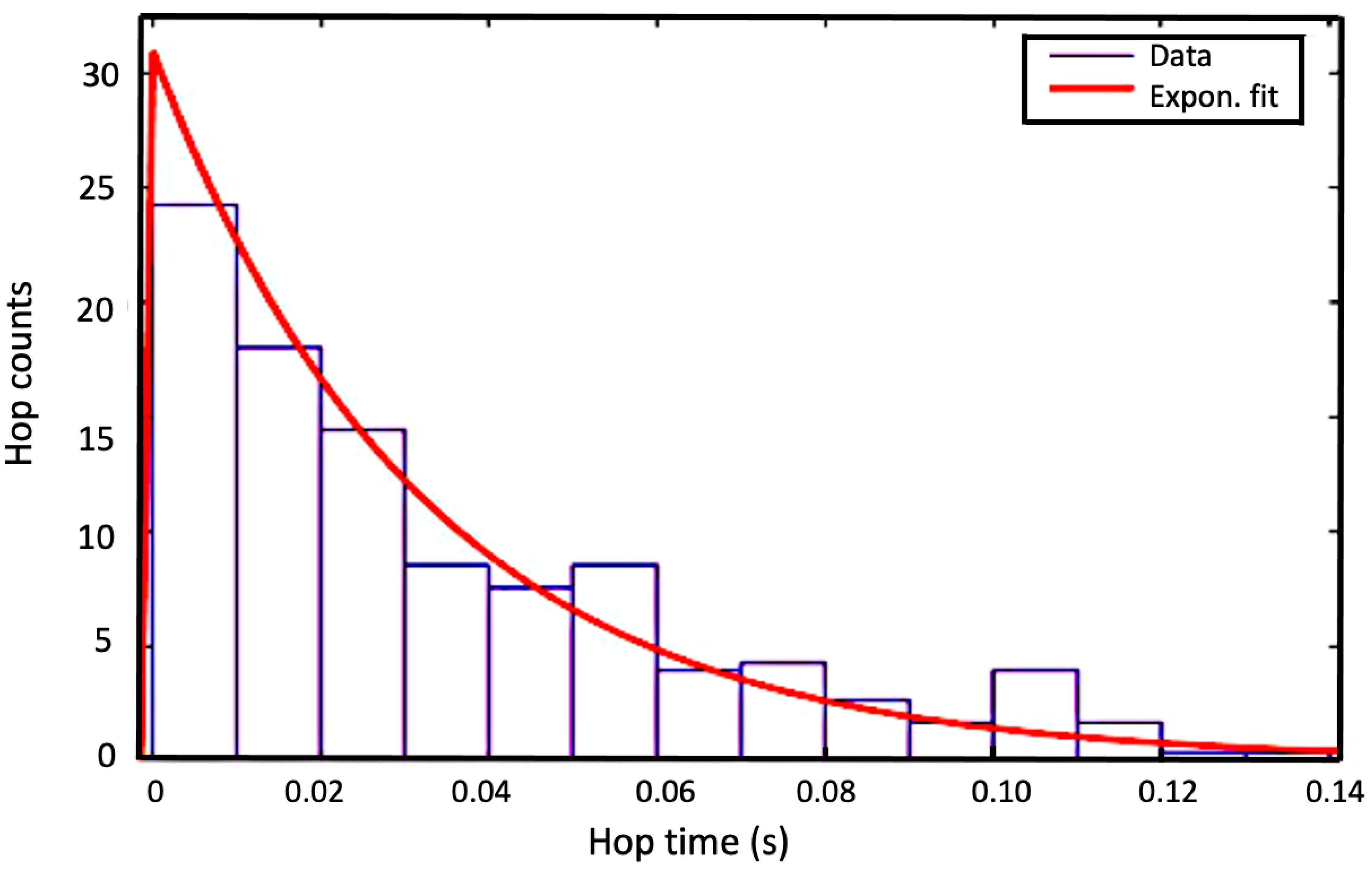
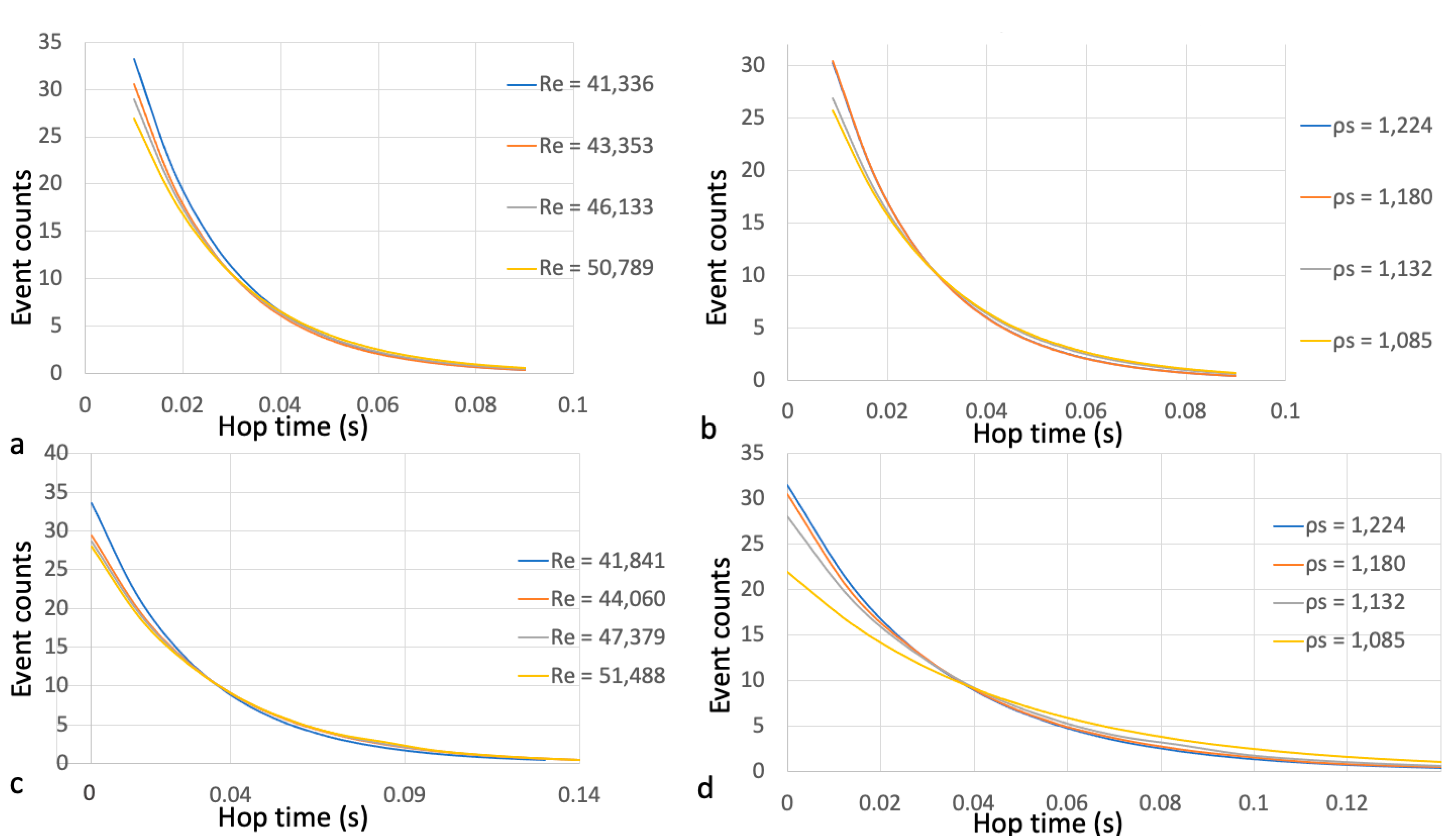
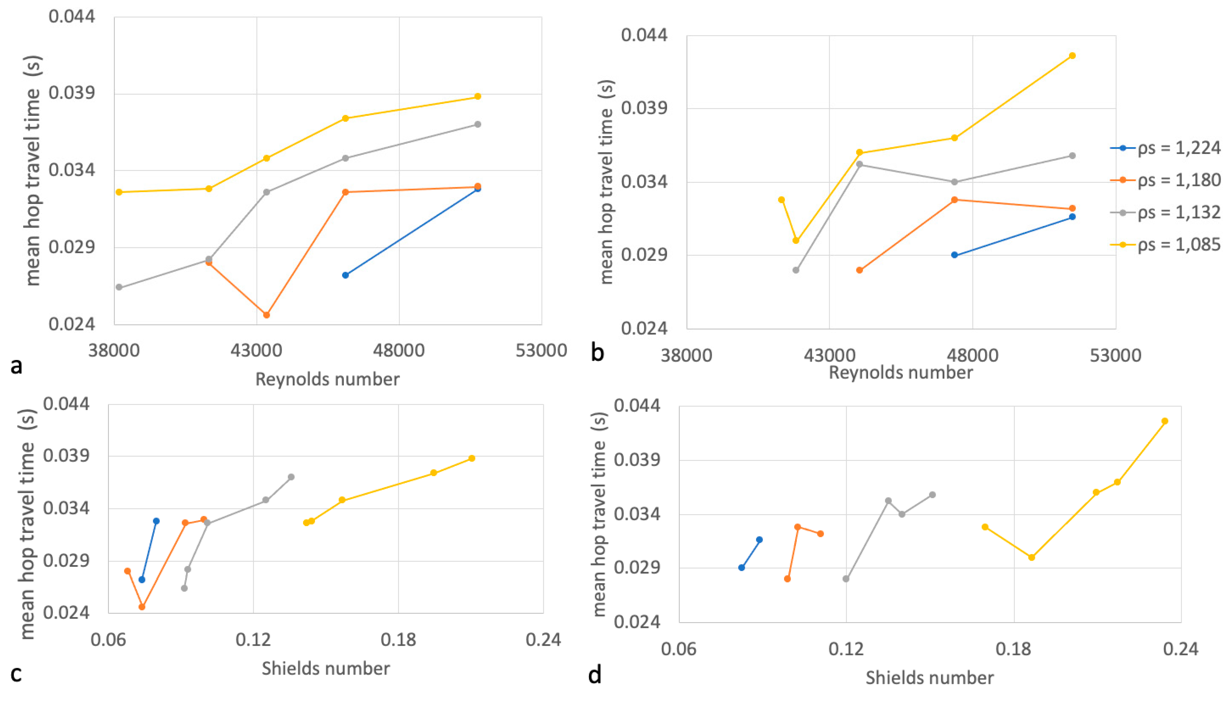
3.2. Hop Travel Time
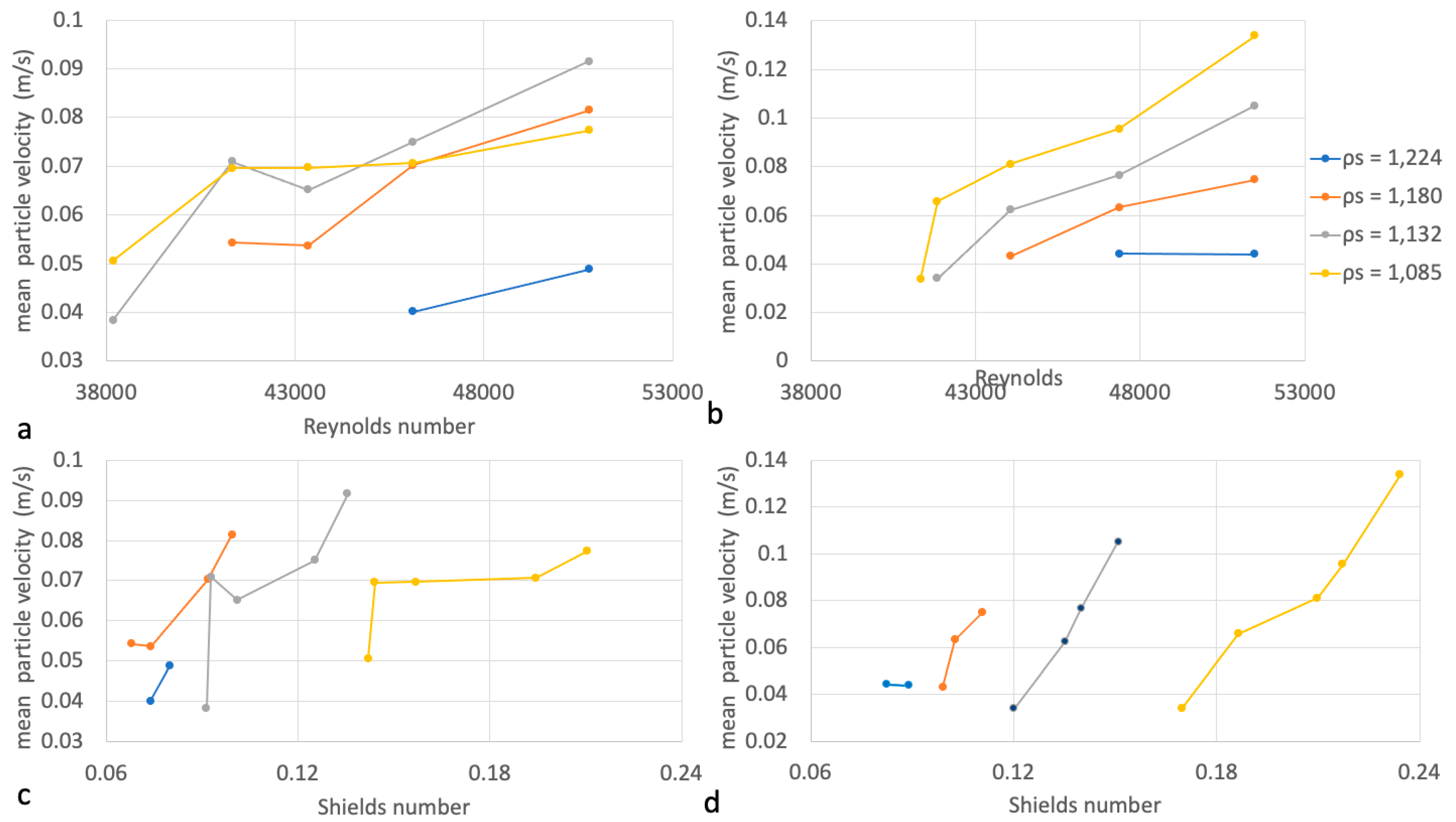
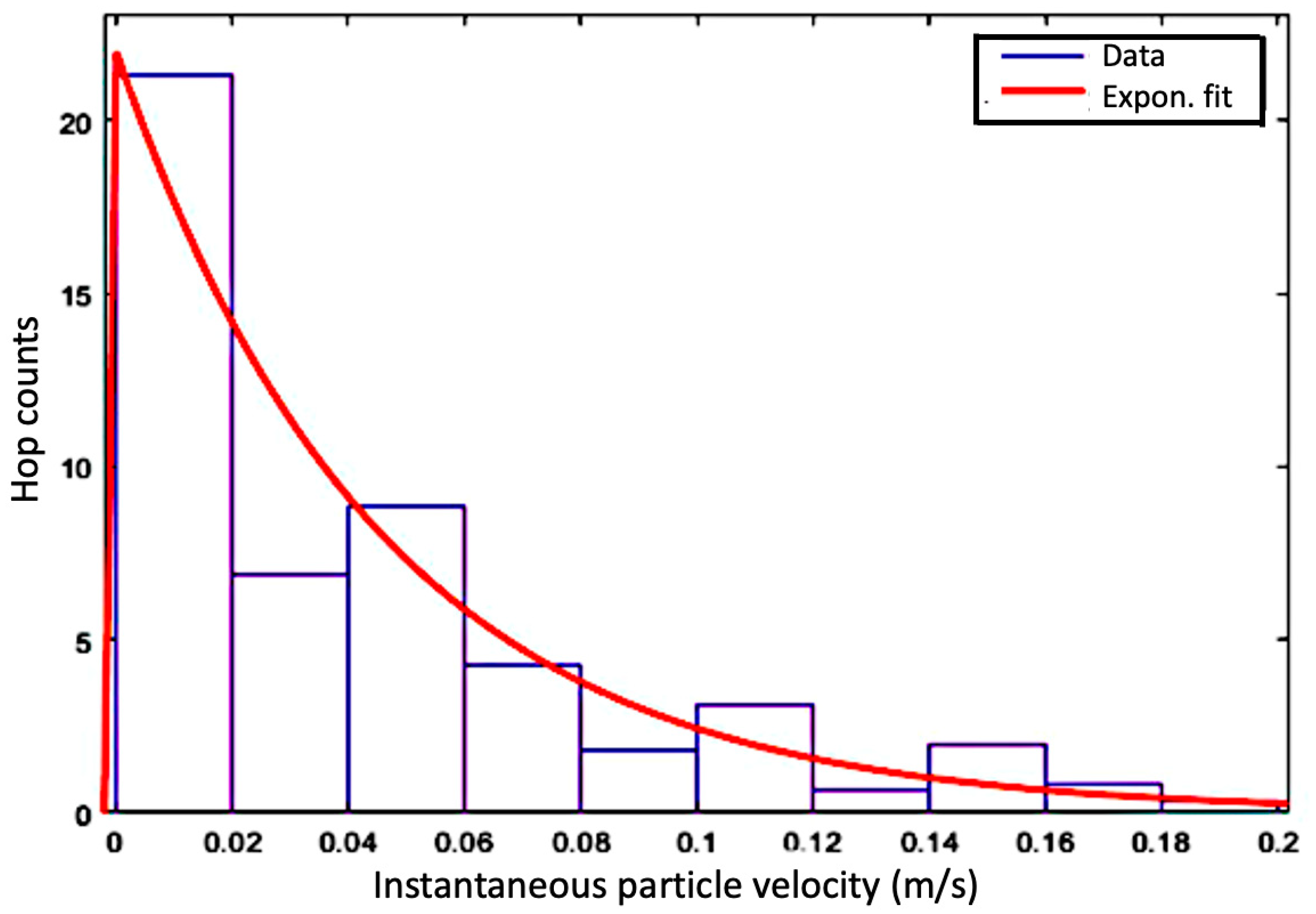
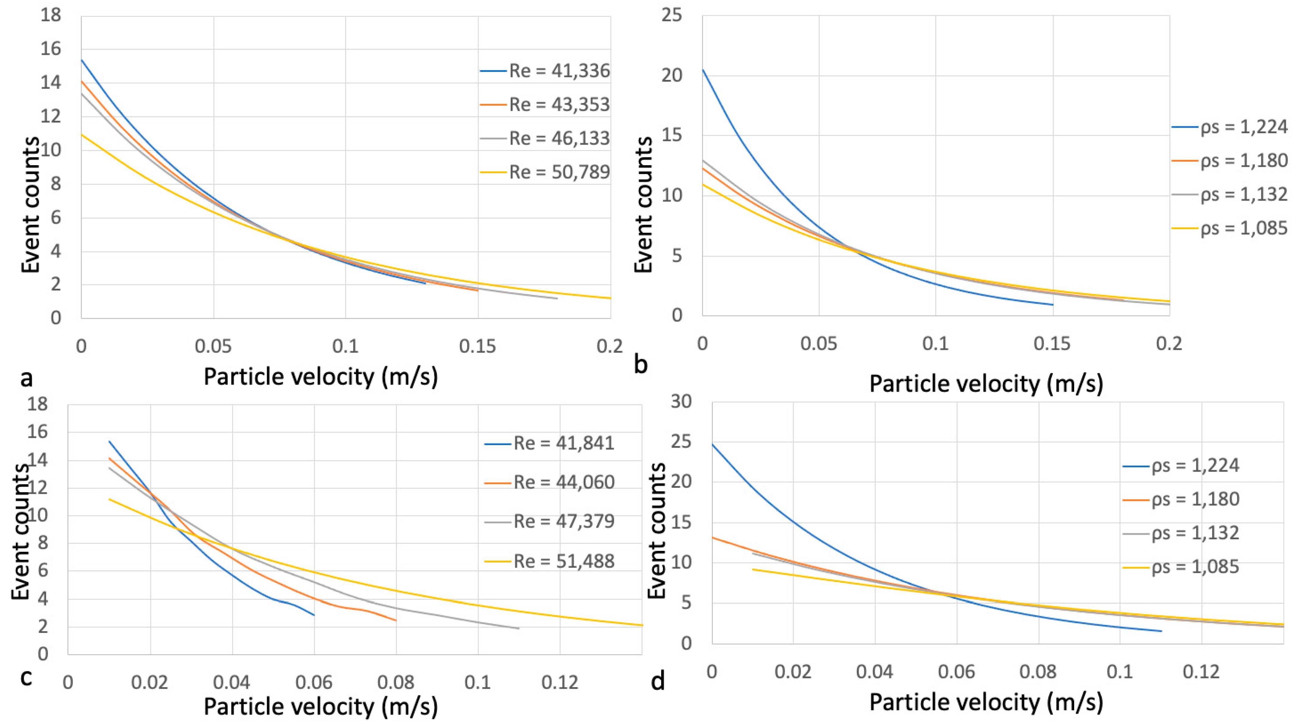
3.3. Particle Velocity
4. Discussion
4.1. Dependence of Hop Travel Distance on Particle and Flow Features
4.2. Dependence of Hop Travel Time on Particle and Flow Features
4.3. Dependence of Particle Velocity on Particle and Flow Features
4.4. Considerations around the Instrumented Particle’s Design
5. Conclusions
Author Contributions
Funding
Institutional Review Board Statement
Informed Consent Statement
Data Availability Statement
Acknowledgments
Conflicts of Interest
Appendix A
Appendix A.1. Dependence of Hop Distances on Particle and Flow Features

| Surface A | Surface B | |||||||
|---|---|---|---|---|---|---|---|---|
| Particle Density (kg/m3) | Particle Density (kg/m3) | |||||||
| 1085 | 1132 | 1180 | 1224 | 1085 | 1132 | 1180 | 1224 | |
| Hop Length (m) | Probability of Occurrence (%) | |||||||
| 0–0.0025 | 47.1 | 65.79 | 67.4 | 67.6 | 43.4 | 65.84 | 65.7 | 69.1 |
| 0.0025–0.005 | 28.8 | 22.55 | 22.6 | 23.4 | 30.1 | 22.56 | 25.4 | 21.9 |
| 0.005–0.0075 | 13.9 | 7.69 | 7.0 | 6.9 | 15.2 | 7.57 | 6.4 | 6.9 |
| 0.0075–0.01 | 6.1 | 2.62 | 2.1 | 1.6 | 6.7 | 2.60 | 1.8 | 1.6 |
| >0.01 | 4.1 | 1.34 | 0.9 | 0.4 | 4.5 | 1.32 | 0.7 | 0.4 |
| Surface A | Surface B | |||||||
|---|---|---|---|---|---|---|---|---|
| Flow Reynolds Number | Flow Reynolds Number | |||||||
| 41,337 | 43,353 | 46,133 | 50,789 | 41,841 | 44,060 | 47,379 | 51,488 | |
| Hop Length (m) | Probability of Occurrence (%) | |||||||
| 0–0.0025 | 66.6 | 66.3 | 65.8 | 57.4 | 64.8 | 65.3 | 65.8 | 37.0 |
| 0.0025–0.005 | 25.4 | 25.1 | 22.9 | 27.7 | 25.8 | 25.1 | 22.6 | 32.1 |
| 0.005–0.0075 | 6.4 | 6.7 | 7.5 | 10.1 | 7.6 | 7.3 | 7.7 | 17.6 |
| 0.0075–0.01 | 1.4 | 1.5 | 2.6 | 3.4 | 1.4 | 1.6 | 2.6 | 8.0 |
| >0.01 | 0.3 | 0.4 | 1.3 | 1.3 | 0.4 | 0.6 | 1.3 | 5.3 |
Appendix A.2. Dependence of Hop Travel Time on Particle and Flow Features
| Surface A | Surface B | |||||||
|---|---|---|---|---|---|---|---|---|
| Particle Density (kg/m3) | Particle Density (kg/m3) | |||||||
| 1085 | 1132 | 1180 | 1224 | 1085 | 1132 | 1180 | 1224 | |
| Hop Travel Time (s) | Probability of Occurrence (%) | |||||||
| 0–0.01 | 30.8 | 31.9 | 34.8 | 35.1 | 27.4 | 32.9 | 35.2 | 36.0 |
| 0.01–0.02 | 21.5 | 21.9 | 22.8 | 22.9 | 20.2 | 22.0 | 22.5 | 23.1 |
| 0.02–0.03 | 15.0 | 15.0 | 14.9 | 14.9 | 14.8 | 15.0 | 15.0 | 14.9 |
| 0.03–0.04 | 10.5 | 10.3 | 9.8 | 9.7 | 10.9 | 10.1 | 9.7 | 9.6 |
| 0.04–0.05 | 7.3 | 7.1 | 6.4 | 6.4 | 8.0 | 6.8 | 6.3 | 6.2 |
| 0.05–0.06 | 5.1 | 4.9 | 4.2 | 4.2 | 5.9 | 4.6 | 4.2 | 4.0 |
| 0.06–0.07 | 3.8 | 3.5 | 2.9 | 2.8 | 4.6 | 3.5 | 2.9 | 2.7 |
| 0.07–0.08 | 2.7 | 2.5 | 1.9 | 1.9 | 3.5 | 2.3 | 2.0 | 1.8 |
| 0.08–0.09 | 1.9 | 1.7 | 1.3 | 1.3 | 2.6 | 1.6 | 1.3 | 1.2 |
| 0.09–0.10 | 1.4 | 1.3 | 0.9 | 0.9 | 2.0 | 1.1 | 0.9 | 0.8 |
| Surface A | Surface B | |||||||
|---|---|---|---|---|---|---|---|---|
| Flow Reynolds Number | Flow Reynolds Number | |||||||
| 41,337 | 43,353 | 46,133 | 50,789 | 41,841 | 44,060 | 47,379 | 51,488 | |
| Hop Travel Time (s) | Probability of Occurrence (%) | |||||||
| 0–0.01 | 35.6 | 34.2 | 33.4 | 32.9 | 35.3 | 35.1 | 33.7 | 31.9 |
| 0.01–0.02 | 23.0 | 22.6 | 22.4 | 22.0 | 23.0 | 22.9 | 22.5 | 21.9 |
| 0.02–0.03 | 14.9 | 15.0 | 15.0 | 15.0 | 14.9 | 14.9 | 15.0 | 15.0 |
| 0.03–0.04 | 9.6 | 9.9 | 10.0 | 10.1 | 9.7 | 9.7 | 10.0 | 10.3 |
| 0.04–0.05 | 6.2 | 6.6 | 6.7 | 6.8 | 6.3 | 6.4 | 6.7 | 7.1 |
| 0.05–0.06 | 4.0 | 4.3 | 4.5 | 4.6 | 4.1 | 4.1 | 4.5 | 4.9 |
| 0.06–0.07 | 2.7 | 3.0 | 3.2 | 3.5 | 2.8 | 2.8 | 3.1 | 3.5 |
| 0.07–0.08 | 1.8 | 2.0 | 2.2 | 2.3 | 1.8 | 1.9 | 2.1 | 2.5 |
| 0.08–0.09 | 1.2 | 1.4 | 1.5 | 1.6 | 1.2 | 1.3 | 1.5 | 1.7 |
| 0.09–0.10 | 0.8 | 1.0 | 1.1 | 1.1 | 0.8 | 0.9 | 1.0 | 1.3 |
Appendix A.3. Dependence of Particle Velocity on Particle and Flow Features
| Surface A | Surface B | |||||||
|---|---|---|---|---|---|---|---|---|
| Particle Density (kg/m3) | Particle Density (kg/m3) | |||||||
| 1085 | 1132 | 1180 | 1224 | 1085 | 1132 | 1180 | 1224 | |
| Hop Velocity (m/s) | Probability of Occurrence (%) | |||||||
| 0–0.015 | 20.3 | 21.1 | 23.0 | 24.4 | 17.3 | 19.3 | 20.6 | 25.1 |
| 0.015–0.03 | 16.7 | 17.1 | 18.1 | 18.8 | 15.5 | 16.1 | 16.8 | 19.1 |
| 0.03–0.045 | 13.7 | 13.8 | 14.2 | 14.5 | 13.3 | 13.4 | 13.7 | 14.6 |
| 0.045–0.06 | 11.2 | 11.2 | 11.2 | 11.1 | 11.4 | 11.1 | 11.2 | 11.1 |
| 0.06–0.075 | 9.2 | 9.1 | 8.8 | 8.6 | 9.9 | 9.3 | 9.1 | 8.5 |
| 0.075–0.09 | 7.5 | 7.3 | 6.9 | 6.6 | 8.3 | 7.7 | 7.5 | 6.4 |
| 0.09–0.105 | 6.2 | 5.9 | 5.4 | 5.1 | 6.9 | 6.4 | 6.1 | 4.9 |
| 0.105–0.12 | 5.0 | 4.8 | 4.3 | 3.9 | 5.7 | 5.3 | 5.0 | 3.7 |
| 0.12–0.135 | 4.1 | 3.9 | 3.4 | 3.0 | 4.7 | 4.5 | 4.0 | 2.8 |
| 0.135–0.15 | 3.4 | 3.2 | 2.7 | 2.3 | 3.8 | 3.7 | 3.3 | 2.2 |
| 0.15–0.165 | 2.8 | 2.6 | 2.1 | 1.8 | 3.1 | 3.1 | 2.7 | 1.7 |
| Surface A | Surface B | |||||||
|---|---|---|---|---|---|---|---|---|
| Flow Reynolds Number | Flow Reynolds Number | |||||||
| 41,337 | 43,353 | 46,133 | 50,789 | 41,841 | 44,060 | 47,379 | 51,488 | |
| Hop Velocity (m/s) | Probability of Occurrence (%) | |||||||
| 0–0.015 | 27.6 | 27.4 | 24.4 | 21.7 | 20.6 | 19.8 | 18.3 | 17.9 |
| 0.015–0.03 | 20.2 | 20.1 | 18.8 | 17.4 | 16.8 | 16.6 | 16.0 | 15.7 |
| 0.03–0.045 | 14.8 | 14.8 | 14.5 | 14.0 | 13.7 | 13.8 | 13.7 | 13.6 |
| 0.045–0.06 | 10.9 | 10.9 | 11.1 | 11.2 | 11.2 | 11.2 | 11.1 | 11.1 |
| 0.06–0.075 | 8.0 | 8.0 | 8.6 | 9.0 | 9.1 | 9.3 | 9.4 | 9.5 |
| 0.075–0.09 | 5.8 | 5.9 | 6.6 | 7.2 | 7.5 | 7.7 | 7.8 | 7.9 |
| 0.09–0.105 | 4.3 | 4.3 | 5.1 | 5.8 | 6.1 | 6.1 | 6.5 | 6.6 |
| 0.105–0.12 | 3.1 | 3.2 | 3.9 | 4.6 | 5.0 | 5.0 | 5.4 | 5.5 |
| 0.12–0.135 | 2.3 | 2.3 | 3.0 | 3.7 | 4.0 | 4.2 | 4.5 | 4.6 |
| 0.135–0.15 | 1.7 | 1.7 | 2.3 | 3.0 | 3.3 | 3.5 | 4.1 | 4.2 |
| 0.15–0.165 | 1.2 | 1.3 | 1.8 | 2.4 | 2.7 | 2.8 | 3.2 | 3.3 |
| Surface A | Surface B | |||||||
|---|---|---|---|---|---|---|---|---|
| Flow Reynolds number (Re) | 41,337 | 43,353 | 46,133 | 50,789 | 41,841 | 44,060 | 47,379 | 51,488 |
| Particle Reynolds number (Re*) | 6149 | 6417 | 6337 | 7433 | 6995 | 7420 | 7552 | 7142 |
References
- Buffington, J.; Montgomery, D. A systematic analysis of eight decades of incipient motion studies, with special reference to gravel-bedded rivers. Water Resour. Res. 1997, 33, 1993–2029. [Google Scholar] [CrossRef] [Green Version]
- Pähtz, T.; Clark, A.H.; Valyrakis, M.; Durán, O. The Physics of Sediment Transport Initiation, Cessation, and Entrainment across Aeolian and Fluvial Environments. Rev. Geophys. 2020, 58, 1–58. [Google Scholar] [CrossRef]
- Bagnold, R.A. An approach to the sediment transport problem from general physics. Physiogr. Hydraul. Stud. Rivers Geol. Surv. Prof. Pap. 1966, 422-I, 1–37. [Google Scholar]
- Bagnold, R.A. Transport of solids by natural water flow: Evidence for a worldwide correlation. Proc. R. Soc. Lond. A Math. Phys. Sci. 1986, 405, 369–374. [Google Scholar]
- Gomez, B.; Church, M. An assessment of bed load sediment transport formulae for gravel bed rivers. Water Resour. Res. 1989, 25, 1161–1186. [Google Scholar] [CrossRef]
- Ancey, C.; Davison, A.C.; Böhm, T.; Jodeau, M.; Frey, P. Entrainment and motion of coarse particles in a shallow water stream down a steep slope. J. Fluid Mech. 2008, 595, 83–114. [Google Scholar] [CrossRef]
- Gimenez-Curto, L.A.; Corniero, M.A. Entrainment threshold of cohesionless sediment grains under steady flow of air and water. Sedimentology 2009, 56, 493–509. [Google Scholar] [CrossRef]
- Wilberg, P.L.; Smith, J.D. Model for calculating bed load transport of sediment. J. Hydraul. Eng. 1989, 115, 101–123. [Google Scholar] [CrossRef]
- Bose, S.T.; Dey, S. Sediment Entrainment Probability and Threshold of Sediment Suspension: Exponential-Based Approach. J. Hydraul. Eng. 2013, 139, 1099–1106. [Google Scholar] [CrossRef]
- Török, G.T.; Józsa, J.; Baranya, S. A Shear Reynolds Number-Based Classification Method of the Nonuniform Bed Load Transport. Water 2019, 11, 73. [Google Scholar] [CrossRef] [Green Version]
- Xiao-Hu, Z.; Valyrakis, M.; Zhen-Shan, L. Rock and roll: Incipient aeolian entrainment of coarse particles. Phys. Fluids 2021, 33, 075117. [Google Scholar] [CrossRef]
- Valyrakis, M.; Diplas, P.; Dancey, C.L.; Greer, K.; Celik, A.O. Role of instantaneous force magnitude and duration on particle entrainment. J. Geophys. Res. Earth Surf. 2010, 115, 1–18. [Google Scholar] [CrossRef]
- Valyrakis, M.; Diplas, P.; Dancey, C.L. Entrainment of coarse grains in turbulent flows: An extreme value theory approach. Water Resour. Res. 2011, 47, 1–17. [Google Scholar] [CrossRef]
- Valyrakis, M.; Diplas, P.; Dancey, C.L. Entrainment of coarse particles in turbulent flows: An energy approach. J. Geophys. Res. Earth Surf. 2013, 118, 42–53. [Google Scholar] [CrossRef] [Green Version]
- Ali, S.Z.; Dey, S. Hydrodynamic instability of meandering channels. Phys. Fluids 2017, 29, 125107. [Google Scholar] [CrossRef]
- Van Rijn, L.C. Sediment transport, part I: Bed load transport. J. Hydraul. Eng. 1984, 110, 1431–1456. [Google Scholar] [CrossRef] [Green Version]
- Garcia, C.; Cohen, H.; Reid, I.; Rovira, A.; Úbeda, X.; Laronne, J.B. Processes of initiation of motion leading to bed load transport in gravel-bed rivers. Geophys. Res. Lett. 2007, 34. [Google Scholar] [CrossRef]
- Drake, T.G.; Shreve, R.L.; Dietrich, W.E.; Whiting, P.J.; Leopold, L.B. Bed load transport of fine gravel observed by motion-picture photography. J. Fluid Mech. 1988, 192, 193–217. [Google Scholar] [CrossRef] [Green Version]
- Cecchetto, M.; Tregnaghi, M.; Bottacin-Busolin, A.; Tait, S.; Marion, A. Statistical description on the role of turbulence and grain interference on particle entrainment from gravel beds. J. Hydraul. Eng. 2017, 143, 06016021. [Google Scholar] [CrossRef] [Green Version]
- Coleman, N. A theoretical and experimental study of drag and lift forces acting on a sphere resting on a hypothetical streambed. In Proceedings of the 12th Congress of International Association for Hydraulic Research, Fort Collins, CO, USA, 11–14 September 1967. [Google Scholar]
- Schmeeckle, M.W.; Nelson, J.M.; Shreve, R.L. Forces on stationary particles in near-bed turbulent flows. J. Geophys. Res. Earth Surf. 2007, 112, 1–21. [Google Scholar] [CrossRef]
- Diplas, P.; Dancey, C.L.; Celik, A.O.; Valyrakis, M.; Greer, K.; Akar, T. The Role of Impulse on the Initiation of Particle Movement under Turbulent Flow Conditions. Science 2008, 322, 717–720. [Google Scholar] [CrossRef] [Green Version]
- Hofland, B.; Battjes, J.A.; Booij, R. Measurement of fluctuating pressures on coarse bed material. J. Hydraul. Eng. 2005, 131, 770–781. [Google Scholar] [CrossRef]
- Jeffreys, H. On the transport of sediments by streams. Math. Proc. Phil. Soc. 1929, 25, 272–276. [Google Scholar] [CrossRef]
- Iwagaki, Y. (I) Hydrodynamical study on critical tractive force. Trans. Jpn. Soc. Civ. Eng. 1956, 41, 1–21. [Google Scholar] [CrossRef] [Green Version]
- Wiberg, P.L.; Smith, J.D. Calculations of the critical shear stress for motion of uniform and heterogeneous sediments. Water Resour. Res. 1987, 23, 1471–1480. [Google Scholar] [CrossRef]
- Hofland, B.; Battjes, J. Probability density function of instantaneous drag forces and shear stresses on a bed. J. Hydraul. Eng. 2006, 132, 1169–1175. [Google Scholar] [CrossRef]
- Campagnol, J.; Radice, A.; Ballio, F.; Nikora, V. Particle motion and diffusion at weak bed load: Accounting for unsteadiness effects of entrainment and disentrainment. J. Hydraul. Res. 2015, 53, 633–648. [Google Scholar] [CrossRef]
- Fathel, S.L.; Furbish, D.J.; Schmeeckle, M.W. Experimental evidence of statistical ensemble behavior in bed load sediment transport. J. Geophys. Res. Earth Surf. 2015, 120, 2298–2317. [Google Scholar] [CrossRef] [Green Version]
- Furbish, D.J.; Schmeeckle, M.W.; Schumer, R.; Fathel, S.L. Probability distributions of bed load particle velocities, accelerations, hop distances, and travel times informed by Jaynes’s principle of maximum entropy. J. Geophys. Res. Earth Surf. 2016, 121, 1373–1390. [Google Scholar] [CrossRef]
- Lajeunesse, E.; Malverti, L.; Charru, F. Bed load transport in turbulent flow at the grain scale: Experiments and modeling. J. Geophys. Res. Earth Surf. 2010, 115. [Google Scholar] [CrossRef]
- Liu, D.; Valyrakis, M.; Williams, R. Flow Hydrodynamics across Open Channel Flows with Riparian Zones: Implications for Riverbank Stability. Water 2017, 9, 720. [Google Scholar] [CrossRef] [Green Version]
- Nasrollahi, A.; Ghodsian, M.; Neyshabouri, S. Local scour at permeable spur dikes. Appl. Sci. 2008, 8, 3398–3406. [Google Scholar] [CrossRef] [Green Version]
- Izadinia, E.; Heidarpour, M.; Schleiss, A. Investigation of turbulence flow and sediment entrainment around a bridge pier. Stoch. Environ. Res. Risk Assess. 2012, 27, 1303–1314. [Google Scholar] [CrossRef] [Green Version]
- Michalis, P.; Tarantino, A.; Tachtatzis, C.; Judd, D.M. Wireless Monitoring of Scour and Re-deposited Sediment Evolution at Bridge Foundations based on Soil Electromagnetic Properties. Smart Mater. Struct. 2015, 24, 1–15. [Google Scholar] [CrossRef] [Green Version]
- Pandey, M.; Valyrakis, M.; Qi, M.; Sharma, A.; Lodhi, A.S. Experimental assessment and prediction of temporal scour depth around a spur dike. Int. J. Sed. Res. 2020, 36, 17–28. [Google Scholar] [CrossRef]
- Papanicolaou, A.; Diplas, P.; Evaggelopoulos, N.; Fotopoulos, S. Stochastic incipient motion criterion for spheres under various bed packing conditions. J. Hydraul. Eng. 2002, 128, 369–380. [Google Scholar] [CrossRef]
- Hassan, M.A.; Voepel, H.; Schumer, R.; Parker, G.; Fraccarollo, L. Displacement characteristics of coarse fluvial bed sediment. J. Geophys. Res. Earth Surf. 2013, 118, 155–165. [Google Scholar] [CrossRef]
- Akeila, E.; Salcic, Z.; Kularatna, N.; Melville, B.; Dwivedi, A. Testing and calibration of smart pebble for river bed sediment transport monitoring. In Proceedings of the IEEE Sensors, Atlanta Georgia, GA, USA, 28–31 October 2007. [Google Scholar]
- Akeila, E.; Salcic, Z. Smart Pebble for Monitoring Riverbed Sediment Transport. IEEE Sens. 2010, 10, 1705–1717. [Google Scholar] [CrossRef]
- Kularatnal, N.; Kularatna-Abeywardana, D. Use of motion sensors for autonomous monitoring of hydraulic environments. In Proceedings of the IEEE Sensors, Lecce, Italy, 26–29 October 2008. [Google Scholar]
- Gronz, O.; Hiller, P.; Wirtz, S.; Becker, K.; Iserloh, T.; Seeger, M.; Brings, C.; Aberle, J.; Casper, M.; Ries, J. Smartstones: A small 9-axis sensor implanted in stones to track their movements. Catena 2016, 142, 245–251. [Google Scholar] [CrossRef] [Green Version]
- Frank, D.; Foster, D.; Sou, I.; Calantoni, J.; Chou, P. Lagrangian measurements of incipient motion in oscillatory flows. J. Geophys. Res. Ocean. 2014, 120, 244–256. [Google Scholar] [CrossRef]
- Maniatis, G.; Hoey, T.; Hassan, M.; Sventek, J.; Hodge, R.; Drysdale, T.; Valyrakis, M. Calculating the Explicit Probability of Entrainment Based on Inertial Acceleration Measurements. J. Hydraul. Eng. 2017, 143, 1–43. [Google Scholar] [CrossRef] [Green Version]
- Noss, C.; Koca, K.; Zinke, P.; Henry, P.H.; Navaratnam, C.U.; Aberle, J.; Lorke, A. A Lagrangian drifter for surveys of water surface roughness in streams. J. Hydraul. Res. 2019, 58, 471–488. [Google Scholar] [CrossRef]
- Valyrakis, M.; Alexakis, A. Development of a “smart-pebble” for tracking sediment transport. In Proceedings of the International Conference on Fluvial Hydraulics, St. Louis, MO, USA, 12–15 July 2016. [Google Scholar]
- Al-Obaidi, K.; Xu, Y.; Valyrakis, M. The Design and Calibration of Instrumented Particles for Assessing Water Infrastructure Hazards. J. Sens. Actuat. Netw. 2020, 9, 36. [Google Scholar] [CrossRef]
- Al-Obaidi, K.; Valyrakis, M. A sensory instrumented particle for environmental monitoring applications: Development and calibration. IEEE Sens. J. 2021, 21, 10153–10166. [Google Scholar] [CrossRef]
- AlObaidi, K.; Valyrakis, M. Explicit linking the probability of entrainment to the flow hydrodynamics. Earth Surface Process. Landf. 2021. [Google Scholar] [CrossRef]
- Bohorquez, P.; Ancey, C. Stochastic-deterministic modeling of bed load transport in shallow water flow over erodible slope: Linear stability analysis and numerical simulation. Adv. Water Resour. 2015, 83, 36–54. [Google Scholar] [CrossRef]
- Einstein, H.A. Bedload Transport as a Probability Problem. Ph.D. Thesis, ETH Zurich, Zurich, Switzerland, 1937. [Google Scholar]
- Yang, C.T.; Sayre, W.W. Stochastic model for sand dispersion. J. Hydraul. Div. ASCE 1971, 97, 265–288. [Google Scholar] [CrossRef]
- Bagnold, R.A. The nature of saltation and of ‘bed-load’transport in water. Proc. R. Soc. Lond. A Math. Phys. Sci. 1973, 332, 473–504. [Google Scholar]
- Shields, A. Application of Similarity Principles and Turbulence Research to Bed-Load Movement; California Institute of Technology: Pasadena, CA, USA, 1936. [Google Scholar]
- Towsend, A.A. The Structure of Turbulent Shear Flow, 2nd ed.; The Press Syndicate of the University of Cambridge: Cambridge, UK, 1980. [Google Scholar]
- Papanicolaou, T.; Knapp, D. A particle tracking technique for bedload motion. In Proceedings of the 7th International Conference on HydroScience and Engineering, Philadelphia, PA, USA, 10–13 September 2006. [Google Scholar]
- Ballio, F.; Pokrajac, D.; Radice, A.; Hosseini-Sadabadi, S.A. Lagrangian and Eulerian description of bed load transport. J. Geophys. Res. Earth Surf. 2018, 123, 384–408. [Google Scholar] [CrossRef]
- Roseberry, J.C.; Schmeeckle, M.W.; Furbish, D.J. A probabilistic description of the bed load sediment flux: 2. Particle activity and motions. J. Geophys. Res. Earth Surf. 2012, 117. [Google Scholar] [CrossRef] [Green Version]
- Schmidt, K.H.; Ergenzinger, P. Bed load entrainment, travel lengths, step lengths, rest periods—Studied with passive (iron, magnetic) and active (radio) tracer techniques. Earth Surf. Proc. Landf. 1992, 17, 147–165. [Google Scholar] [CrossRef]
- Lamarre, H.; Roy, A.G. A field experiment on the development of sedimentary structures in a gravel-bed river. Earth Surf. Proc. Landf. 2008, 33, 1064–1081. [Google Scholar] [CrossRef]
- Hassan, M.A.; Church, M.; Schick, A.P. Distance of movement of coarse particles in gravel bed streams. Water Resour. Res. 1991, 27, 503–511. [Google Scholar] [CrossRef]
- Habersack, H. Radio-tracking gravel particles in a large braided river in New Zealand: A field test of the stochastic theory of bed load transport proposed by Einstein. Hydrol. Proc. 2001, 15, 377–391. [Google Scholar] [CrossRef]
- Nakagawa, H.; Tsujimoto, T. Sand bed instability due to bed load motion. J. Hydraul. Div. ASCE 1980, 106, 2029–2051. [Google Scholar] [CrossRef]
- Martin, R.L.; Jerolmack, D.J.; Schumer, R. The physical basis for anomalous diffusion in bed load transport. J. Geophys. Res. Earth Surf. 2012, 117. [Google Scholar] [CrossRef] [Green Version]
- Ancey, C.; Heyman, J. A microstructural approach to bed load transport: Mean behaviour and fluctuations of particle transport rates. J. Fluid Mech. 2014, 744, 129–168. [Google Scholar] [CrossRef] [Green Version]
- Heays, K.; Friedrich, H.; Melville, B.; Nokes, R. Quantifying the dynamic evolution of graded gravel beds using particle tracking velocimetry. J. Hydraul. Eng. 2014, 140, 04014027. [Google Scholar] [CrossRef]
- Hosseini-Sadabadi, S.A. Langragian and Eulerian Study of Bed-Load Kinematics. Ph.D. Thesis, Politecnico di Milano, Milan, Italy, 2017. [Google Scholar]
- Curley, E.A.M.; Valyrakis, M.; Thomas, R.; Adams, C.E.; Stephen, A. Smart sensors to predict entrainment of freshwater mussels: A new tool in freshwater habitat assessment. Sci. Total Environ. 2021, 787, 1–11. [Google Scholar] [CrossRef]
- Nichols, M. A radio frequency identification system for monitoring coarse sediment particle displacement. Appl. Eng. Agric. 2004, 20. [Google Scholar] [CrossRef] [Green Version]
- MacVicar, B.J.; Piégay, H.; Henderson, A.; Comiti, F.; Oberlin, C.; Pecorari, E. Quantifying the temporal dynamics of wood in large rivers: Field trials of wood surveying, dating, tracking, and monitoring techniques. Earth Surf. Proc. Landf. 2009, 34, 2031–2046. [Google Scholar] [CrossRef]
- Liébault, F.; Hervé, B.; Chapuis, M.; Klotz, S.; Deschâtres, M. Bedload tracing in a high-sediment-load mountain stream. Earth Surf. Proc. Landf. 2011, 37, 385–399. [Google Scholar] [CrossRef]
- Miller, I.M.; Warrick, J.A. Measuring sediment transport and bed disturbance with tracers on a mixed beach. Mar. Geol. 2012, 299–302, 1–17. [Google Scholar] [CrossRef]
- Diplas, P.; Celik, A.O.; Valyrakis, M.; Dancey, C.L. Some Thoughts on Measurements of Marginal Bedload Transport Rates Based on Experience from Laboratory Flume Experiments. US Geol. Surv. Sci. Investig. Rep. 2010, 5091, 130–142. [Google Scholar]


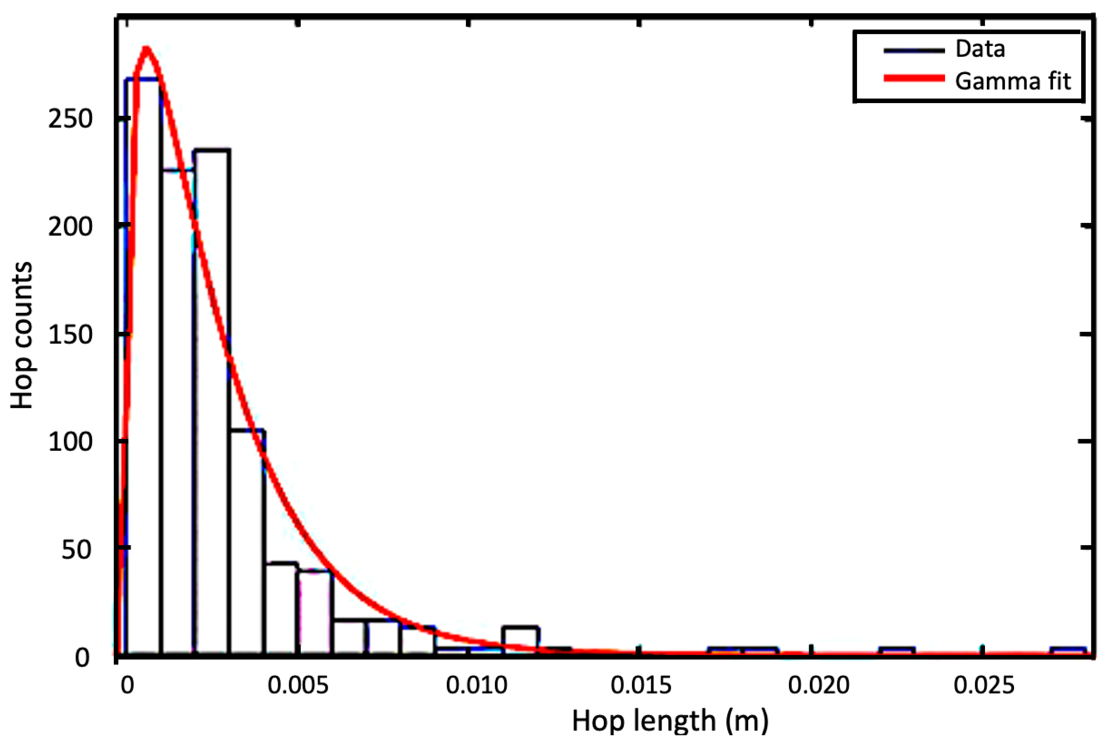


| Model Distribution for Travel Distances | Goodness of Fit (for Q = 56 L/s) | Goodness of Fit (for Q = 42 L/s) | Rank |
|---|---|---|---|
| Weibull | 1.28 | 1.64 | 2 |
| Beta | 3.54 | 1.92 | 3 |
| Gamma | 0.34 | 0.58 | 1 |
| Normal | 3.7 | 5.2 | 4 |
| Exponential | 6.4 | 7.1 | 5 |
| Model Distribution for Travel Times | Goodness of Fit (for Q = 56 L/s) | Goodness of Fit (for Q = 42 L/s) | Rank |
|---|---|---|---|
| Weibull | 4.1 | 4.6 | 4 |
| Beta | 3.2 | 2.8 | 3 |
| Gamma | 6.4 | 7.1 | 5 |
| Normal | 1.4 | 1.8 | 2 |
| Exponential | 0.4 | 0.6 | 1 |
| Model Distribution for Particle Velocities | Goodness of Fit (for Q = 56 L/s) | Goodness of Fit (for Q = 42 L/s) | Rank |
|---|---|---|---|
| Weibull | 4.4 | 4.7 | 4 |
| Beta | 2.9 | 3.1 | 3 |
| Gamma | 5.6 | 6.2 | 5 |
| Normal | 1.7 | 2.1 | 2 |
| Exponential | 0.6 | 0.7 | 1 |
Publisher’s Note: MDPI stays neutral with regard to jurisdictional claims in published maps and institutional affiliations. |
© 2021 by the authors. Licensee MDPI, Basel, Switzerland. This article is an open access article distributed under the terms and conditions of the Creative Commons Attribution (CC BY) license (https://creativecommons.org/licenses/by/4.0/).
Share and Cite
Alhusban, Z.; Valyrakis, M. Assessing and Modelling the Interactions of Instrumented Particles with Bed Surface at Low Transport Conditions. Appl. Sci. 2021, 11, 7306. https://doi.org/10.3390/app11167306
Alhusban Z, Valyrakis M. Assessing and Modelling the Interactions of Instrumented Particles with Bed Surface at Low Transport Conditions. Applied Sciences. 2021; 11(16):7306. https://doi.org/10.3390/app11167306
Chicago/Turabian StyleAlhusban, Zaid, and Manousos Valyrakis. 2021. "Assessing and Modelling the Interactions of Instrumented Particles with Bed Surface at Low Transport Conditions" Applied Sciences 11, no. 16: 7306. https://doi.org/10.3390/app11167306
APA StyleAlhusban, Z., & Valyrakis, M. (2021). Assessing and Modelling the Interactions of Instrumented Particles with Bed Surface at Low Transport Conditions. Applied Sciences, 11(16), 7306. https://doi.org/10.3390/app11167306