
Low Ionosphere under Influence of Strong Solar Radiation: Diagnostics and Modeling


Abstract
:Featured Application
Abstract
1. Introduction
2. Methods
2.1. VLF Technique for Monitoring Low Altitude Ionosphere
2.2. Simulated VLF Signals
2.3. Procedure for Determination of Electron Density: Two-Component Exponential Model
3. Results
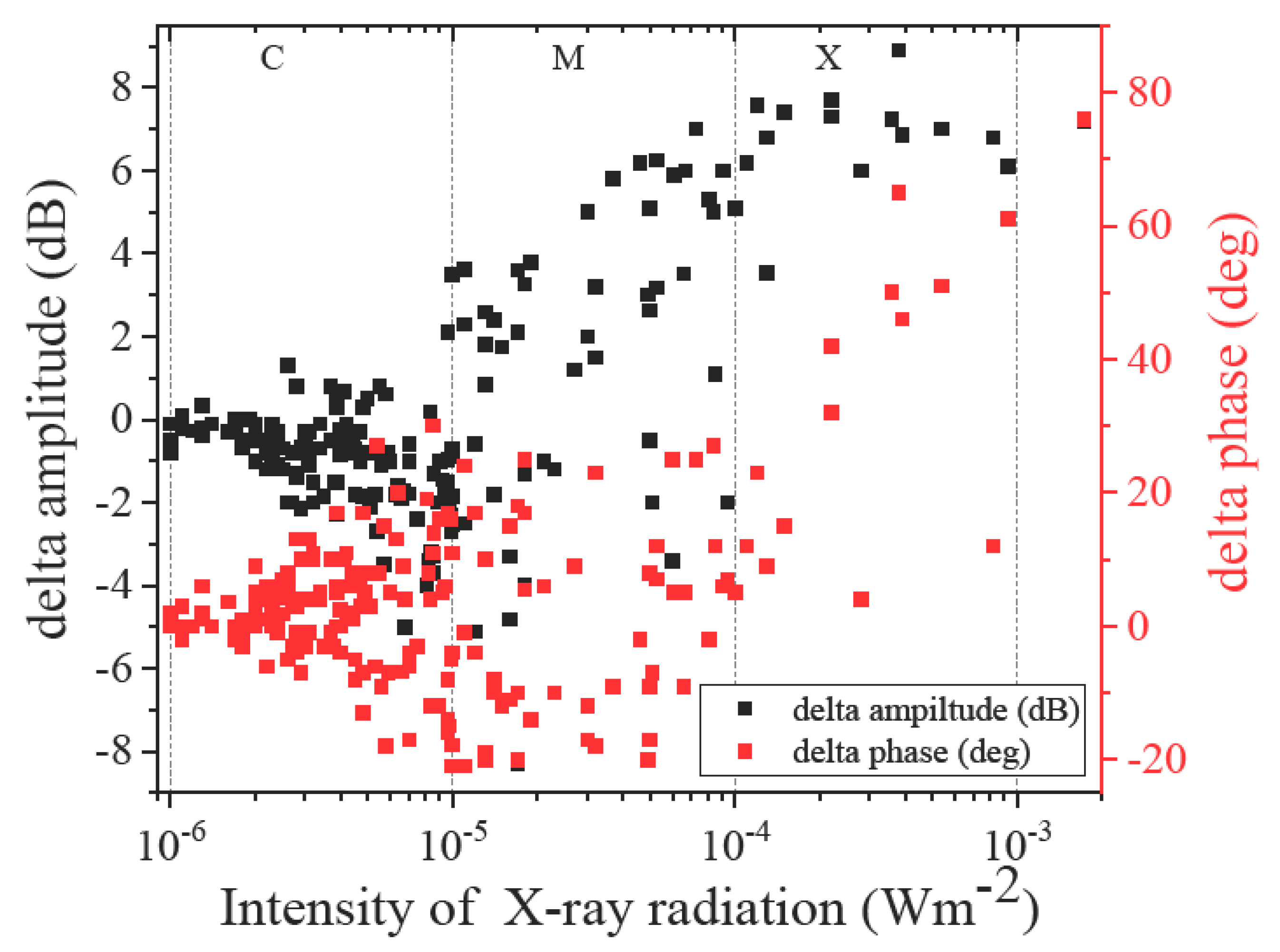
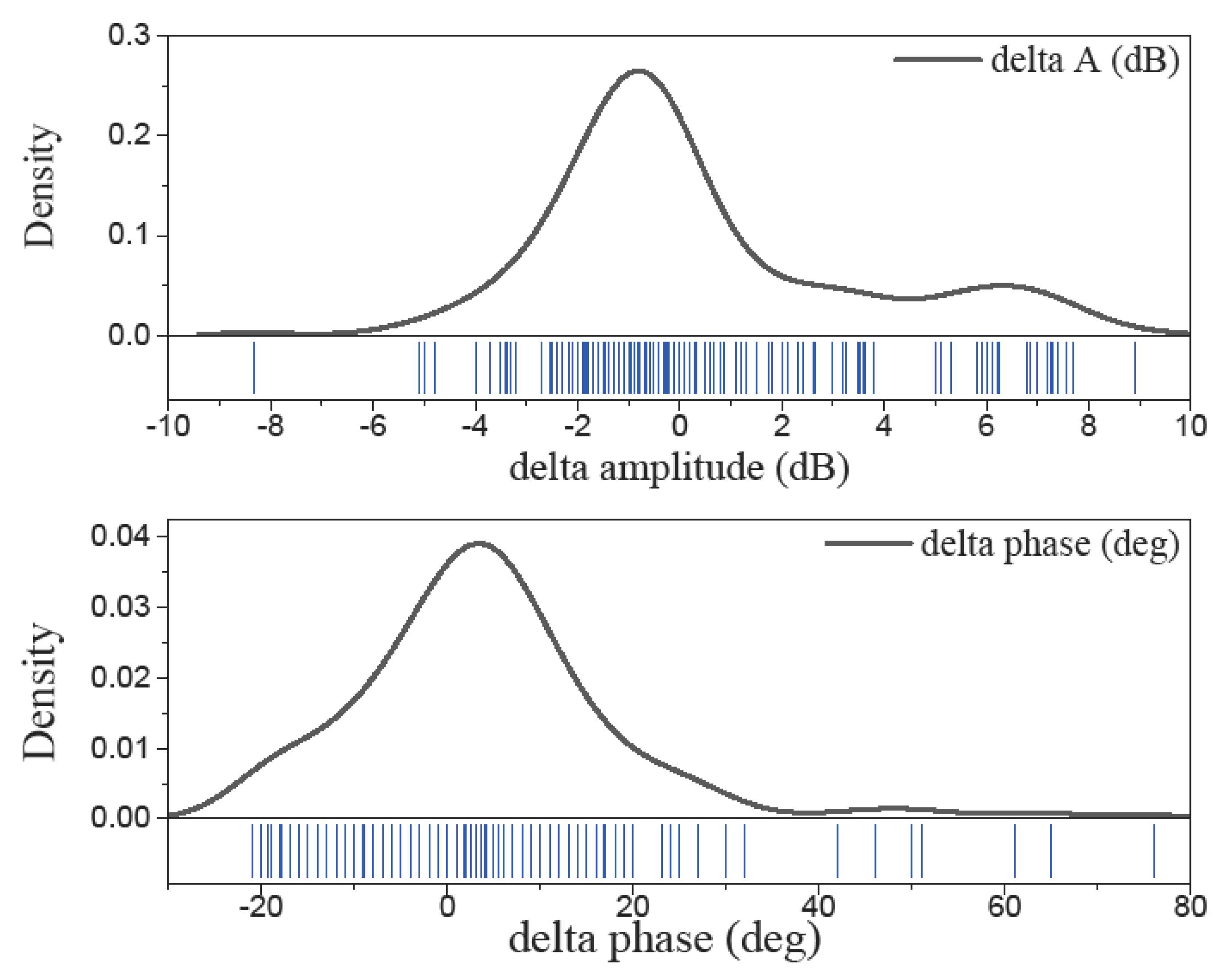
3.1. Recorded Variations of VLF Amplitude and Phase Data
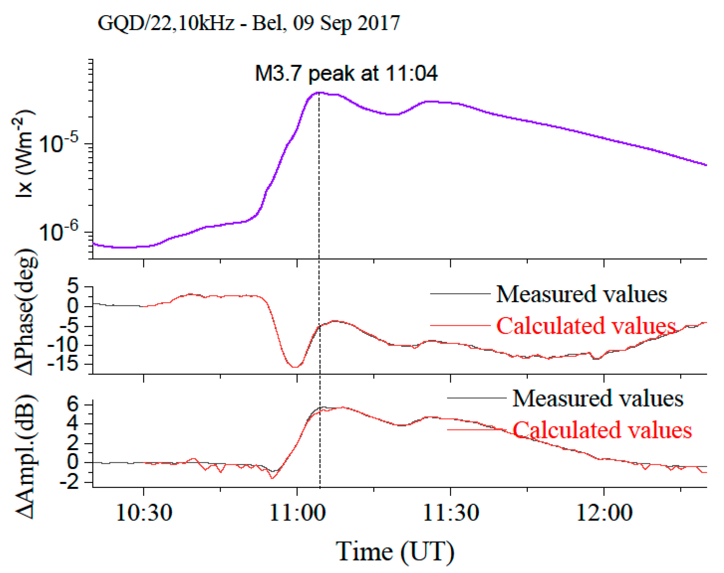
3.2. Long Lasting Intense Solar Radiation: An Analysis of Strong SF
3.3. Intense Solar Radiation: Consecutive Strong SF
3.4. Approximative Expressions
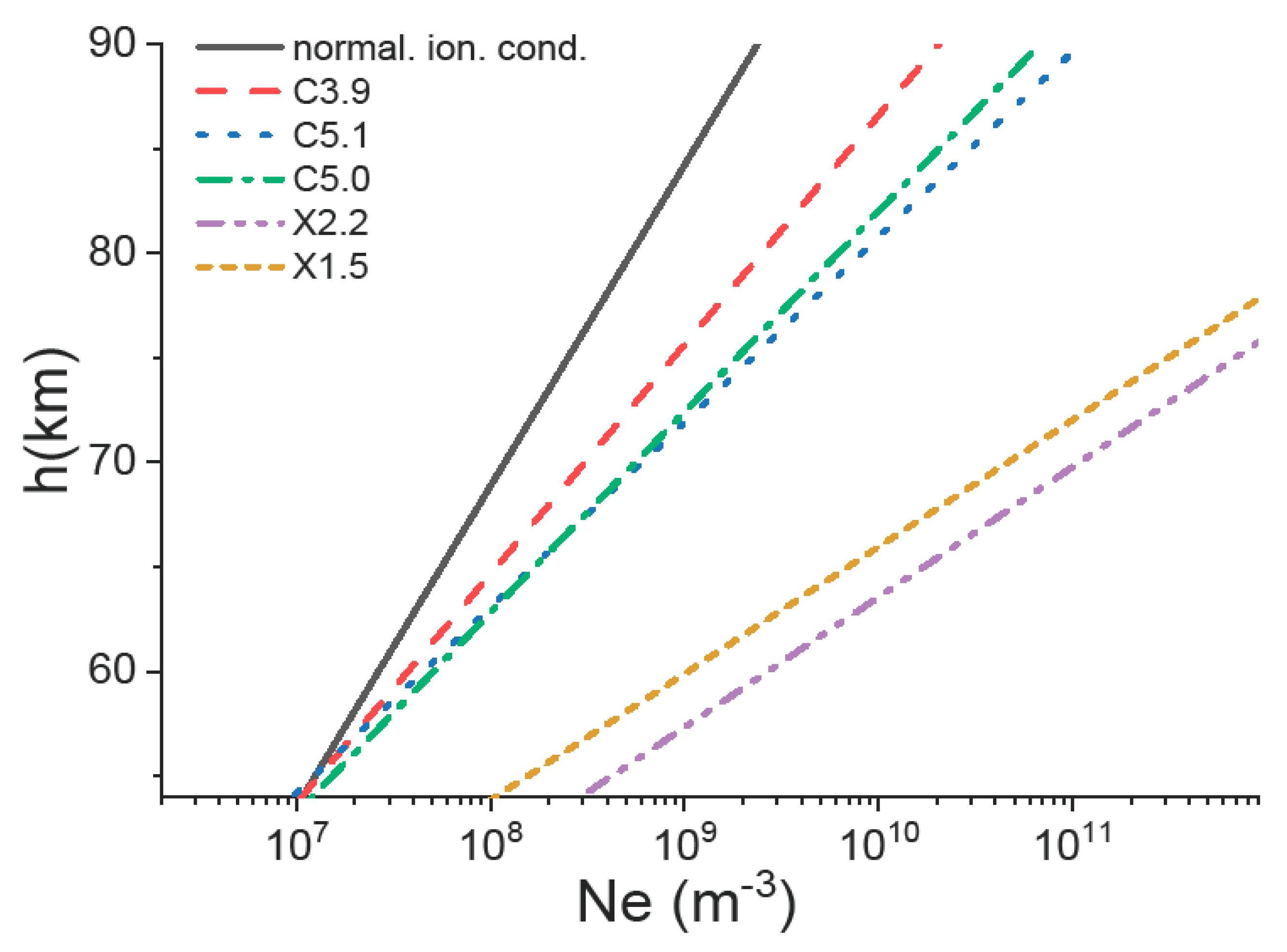
3.5. Comparison of Obtained Ionospheric Parameters
4. Discussion and Conclusions
Supplementary Materials
Author Contributions
Funding
Data Availability Statement
Acknowledgments
Conflicts of Interest
References
- Ravishankara, A.R.; Solomon, S.; Turnipseed, A.A.; Warren, R.F. Atmospheric lifetimes of long-lived halogenated species. Science 1993, 259, 194–199. [Google Scholar] [CrossRef] [Green Version]
- Reid, G.C. Ion Chemistry in the D Region; Academic Press: Cambridge, MA, USA, 1976; Volume 12, pp. 375–413. [Google Scholar]
- Torkar, K.M.; Friedrich, M. Tests of an ion-chemical model of the D-and lower E-region. J. Atmos. Sol. Terr. Phys. 1983, 45, 369–385. [Google Scholar] [CrossRef]
- Turunen, E.; Matveinen, H.; Tolvanen, J.; Ranta, H. D-Region ion Chemistry Model; Utah State University: Logan, UT, USA, 1996; pp. 1–25. [Google Scholar]
- Kelley, M.C. The Earth’s Ionosphere: Plasma Physics and Electrodynamics, Ser. International Geophysics, 2nd ed.; Academic press: San Diego, CA, USA, 2009. [Google Scholar]
- Prölss, G. Physics of the Earth’s Space Environment: An Introduction; Springer Science & Business Media: Berlin/Heidelberg, Germany, 2004. [Google Scholar]
- Barta, V.; Haldoupis, C.; Sátori, G.; Buresova, D.; Chum, J.; Pozoga, M.; Berényi, K.A.; Bór, J.; Popek, M.; Kis, Á. Searching for effects caused by thunderstorms in midlatitude sporadic E layers. J. Atmos. Sol. Terr. Phys. 2017, 161, 150–159. [Google Scholar] [CrossRef] [Green Version]
- Brasseur, G.P.; Solomon, S. Aeronomy of the Middle Atmosphere: Chemistry and Physics of the Stratosphere and Mesosphere, 3rd ed.; Springer Science & Business Media: Dordrecht, The Netherlands, 2005; Volume 32. [Google Scholar]
- Mitra, A.P. Ionospheric Effects of Solar Flares; Springer: Dordrecht, The Netherlands, 1974. [Google Scholar] [CrossRef]
- Nicolet, M.; Aikin, A.C. The formation of the D region of the ionosphere. J. Geophys. Res. 1960, 65, 1469–1483. [Google Scholar] [CrossRef]
- Nina, A.; Čadež, V.M.; Popović, L.Č.; Srećković, V.A. Diagnostics of plasma in the ionospheric D-region: Detection and study of different ionospheric disturbance types. Eur. Phys. J. D 2017, 71, 1–12. [Google Scholar] [CrossRef] [Green Version]
- Cannon, P.; Angling, M.; Barclay, L.; Curry, C.; Dyer, C.; Edwards, R.; Greene, G.; Hapgood, M.; Horne, R.; Jackson, D.; et al. Extreme Space Weather: Impacts on Engineered Systems and Infrastructure; Royal Academy of Engineering: London, UK, 2013. [Google Scholar]
- Kappenman, J.G. Geomagnetic Disturbances and Impacts upon Power System Operation, in Electric Power Generation, Transmission, and Distribution, 3rd ed.; CRC Press: Boca Raton, FL, USA, 2012; Volume 16, pp. 1–22. [Google Scholar]
- Mannucci, A.J.; Tsurutani, B.T.; Iijima, B.A.; Komjathy, A.; Saito, A.; Gonzalez, W.D.; Guarnieri, F.L.; Kozyra, J.U.; Skoug, R. Dayside global ionospheric response to the major interplanetary events of October 29–30, 2003 “Halloween Storms”. Geophys. Res. Lett. 2005, 32, L12S02. [Google Scholar] [CrossRef] [Green Version]
- McMorrow, D. Impacts of Severe Space Weather on the Electric Grid; JASON: Washington, VA, USA, 2011; pp. 22102–27508. [Google Scholar]
- Bondur, V.G.; Pulinets, S.A.; Kim, G.A. Role of variations in galactic cosmic rays in tropical cyclogenesis: Evidence of Hurricane Katrina. Dokl. Earth Sci. 2008, 422, 1124. [Google Scholar] [CrossRef]
- Radovanović, M.M.; Vyklyuk, Y.; Stevančević, M.T.; Milenković, M.Đ.; Jakovljević, D.M.; Petrović, M.D.; Malinović-Milićević, S.B.; Vuković, N.; Vujko, A.Đ.; Yamashkin, A. Forest fires in Portugal-case study, 18 June 2017. Therm. Sci. 2019, 23, 73–86. [Google Scholar] [CrossRef] [Green Version]
- Vyklyuk, Y.; Radovanović, M.M.; Stanojević, G.; Petrović, M.D.; Ćurčić, N.B.; Milenković, M.; Malinović, M.S.; Milovanović, B.; Yamashkin, A.A.; Milanović, P.A. Connection of Solar Activities and Forest Fires in 2018: Events in the USA (California), Portugal and Greece. Sustainability 2020, 12, 10261. [Google Scholar] [CrossRef]
- Barr, R. The propagation of ELF and VLF radio waves beneath an inhomogeneous anisotropic ionosphere. J. Atmos. Sol. Terr. Phys. 1971, 33, 343–353. [Google Scholar] [CrossRef]
- Vinkovic, D.; Gritsevich, M.; Srećković, V.; Pecnik, B.; Szabó, G.; Debattista, V.; Skoda, P.; Mahabal, A.; Peltoniemi, J.; Mönkölä, S. Big data era in meteor science. In Proceedings of the International Meteor Conference, Egmond, The Netherlands, 2–5 June 2016; pp. 319–329. [Google Scholar]
- Nina, A.; Čadež, V.; Srećković, V.; Šulić, D. The influence of solar spectral lines on electron concentration in terrestrial ionosphere. Open Astron. 2011, 20, 609–612. [Google Scholar] [CrossRef] [Green Version]
- Šulić, D.; Srećković, V. A comparative study of measured amplitude and phase perturbations of VLF and LF radio signals induced by solar flares. Serb. Astron. J. 2014, 188, 45–54. [Google Scholar] [CrossRef] [Green Version]
- AWESOME. Receiver. Available online: http://solar-center.stanford.edu/SID/AWESOME (accessed on 30 June 2021).
- Scherrer, D.; Cohen, M.; Hoeksema, T.; Inan, U.; Mitchell, R.; Scherrer, P. Distributing space weather monitoring instruments and educational materials worldwide for IHY 2007: The AWESOME and SID project. Adv. Space Res. 2008, 42, 1777–1785. [Google Scholar] [CrossRef]
- List of VLF Transmitters. Available online: https://en.wikipedia.org/wiki/List_of_VLF-transmitters (accessed on 30 June 2021).
- Šulić, D.; Srećković, V.; Mihajlov, A. A study of VLF signals variations associated with the changes of ionization level in the D-region in consequence of solar conditions. Adv. Space Res. 2016, 57, 1029–1043. [Google Scholar] [CrossRef] [Green Version]
- Ferguson, A.J. Computer Programs for Assessment of Long-Wavelength Radio Communications, Version 2.0: User’s Guide and Source Files; Space and Naval Warfare System Center: San Diego, CA, USA, 1998. [Google Scholar]
- Cohen, M.B.; Inan, U.S.; Paschal, E.W. Sensitive broadband ELF/VLF radio reception with the AWESOME instrument. IEEE Trans. Geosci. Remote. Sens. 2009, 48, 3–17. [Google Scholar] [CrossRef]
- Nina, A.; Čadež, V.; Srećković, V.; Šulić, D. Altitude distribution of electron concentration in ionospheric D-region in presence of time-varying solar radiation flux. Nucl. Instrum. Methods Phys. Res. B 2012, 279, 110–113. [Google Scholar] [CrossRef] [Green Version]
- LWPC. Computer Programs for Assessment of Long-Wavelength Radio Communications, V2.1. Available online: https://github.com/space-physics/LWPC (accessed on 30 June 2021).
- Morfitt, D.G.; Shellman, C.H. ‘MODESRCH’, An Improved Computer Program for Obtaining ELF/VLF/LF Mode Constants in an Earth-Ionosphere Waveguide; Naval Electronics lab Center: San Diego CA, USA, 1976. [Google Scholar]
- Marshall, R.A.; Wallace, T.; Turbe, M. Finite-difference modeling of very-low-frequency propagation in the earth-ionosphere waveguide. IEEE Trans. Antennas Propag. 2017, 65, 7185–7197. [Google Scholar] [CrossRef]
- Thomson, N.R.; Clilverd, M.A. Solar flare induced ionospheric D-region enhancements from VLF amplitude observations. J. Atmos. Solar Terr. Phys. 2001, 63, 1729–1737. [Google Scholar] [CrossRef]
- Wait, J.R.; Spies, K.P. Characteristics of the Earth-Ionosphere Waveguide for VLF Radio Waves, Technical Note 300; US Department of Commerce, National Bureau of Standards: Boulder, CO, USA, 1964. [Google Scholar]
- Lay, E.H.; Shao, X.M.; Jacobson, A.R. D region electron profiles observed with substantial spatial and temporal change near thunderstorms. J. Geophys. Res. 2014, 119, 4916–4928. [Google Scholar] [CrossRef]
- Garcia, H.A. Temperature and emission measure from GOES soft X-ray measurements. Sol. Phys. 1994, 154, 275–308. [Google Scholar] [CrossRef]
- GOES. Satellite. Available online: https://satdat.ngdc.noaa.gov/sem/goes/data/ (accessed on 30 January 2021).
- GOES-15. X-ray Flux. Available online: https://www.swpc.noaa.gov/products/goes-x-ray-flux (accessed on 30 June 2021).
- Nina, A.; Čadež, V.; Šulić, D.; Srećković, V.; Žigman, V. Effective electron recombination coefficient in ionospheric D-region during the relaxation regime after solar flare from 18 February 2011. Nucl. Instrum. Methods Phys. Res. B 2012, 279, 106–109. [Google Scholar] [CrossRef] [Green Version]
- Ratcliffe, J.A. An Introduction to Ionosphere and Magnetosphere; CUP Archive: Cambridge, UK, 1972. [Google Scholar]
- Pandey, U.; Singh, B.; Singh, O.; Saraswat, V. Solar flare induced ionospheric D-region perturbation as observed at a low latitude station Agra, India. Astrophys. Space Sci. 2015, 357, 1–11. [Google Scholar] [CrossRef]
- Grubor, D.; Šulić, D.; Žigman, V. Classification of X-ray solar flares regarding their effects on the lower ionosphere electron density profile. Ann. Geophys. 2008, 26, 1731–1740. [Google Scholar] [CrossRef] [Green Version]
- Thomson, N.R.; Rodger, C.J.; Clilverd, M.A. Large solar flares and their ionospheric D region enhancements. J. Geophys. Res. 2005, 110, A6. [Google Scholar] [CrossRef] [Green Version]
- Gavrilov, B.; Ermak, V.; Lyakhov, A.; Poklad, Y.V.; Rybakov, V.; Ryakhovsky, I. Reconstruction of the Parameters of the Lower Midlatitude Ionosphere in M-and X-Class Solar Flares. Geomagn. Aeron. 2020, 60, 747–753. [Google Scholar] [CrossRef]
- Jokar Arsanjani, J.; Vaz, E. Special Issue Editorial: Earth Observation and Geoinformation Technologies for Sustainable Development. Sustainability 2017, 9, 760. [Google Scholar] [CrossRef] [Green Version]
- Zhima, Z.; Hu, Y.; Shen, X.; Chu, W.; Piersanti, M.; Parmentier, A.; Zhang, Z.; Wang, Q.; Huang, J.; Zhao, S.; et al. Storm-Time Features of the Ionospheric ELF/VLF Waves and Energetic Electron Fluxes Revealed by the China Seismo-Electromagnetic Satellite. Appl. Sci. 2021, 11, 2617. [Google Scholar] [CrossRef]


| Time [UT] | SID VLF Data at Peak Time | ||||||
|---|---|---|---|---|---|---|---|
| SF | Start | Peak | End | ΔA [dB] | ΔP [deg] | Ix max XL [Wm−2] | Active Region |
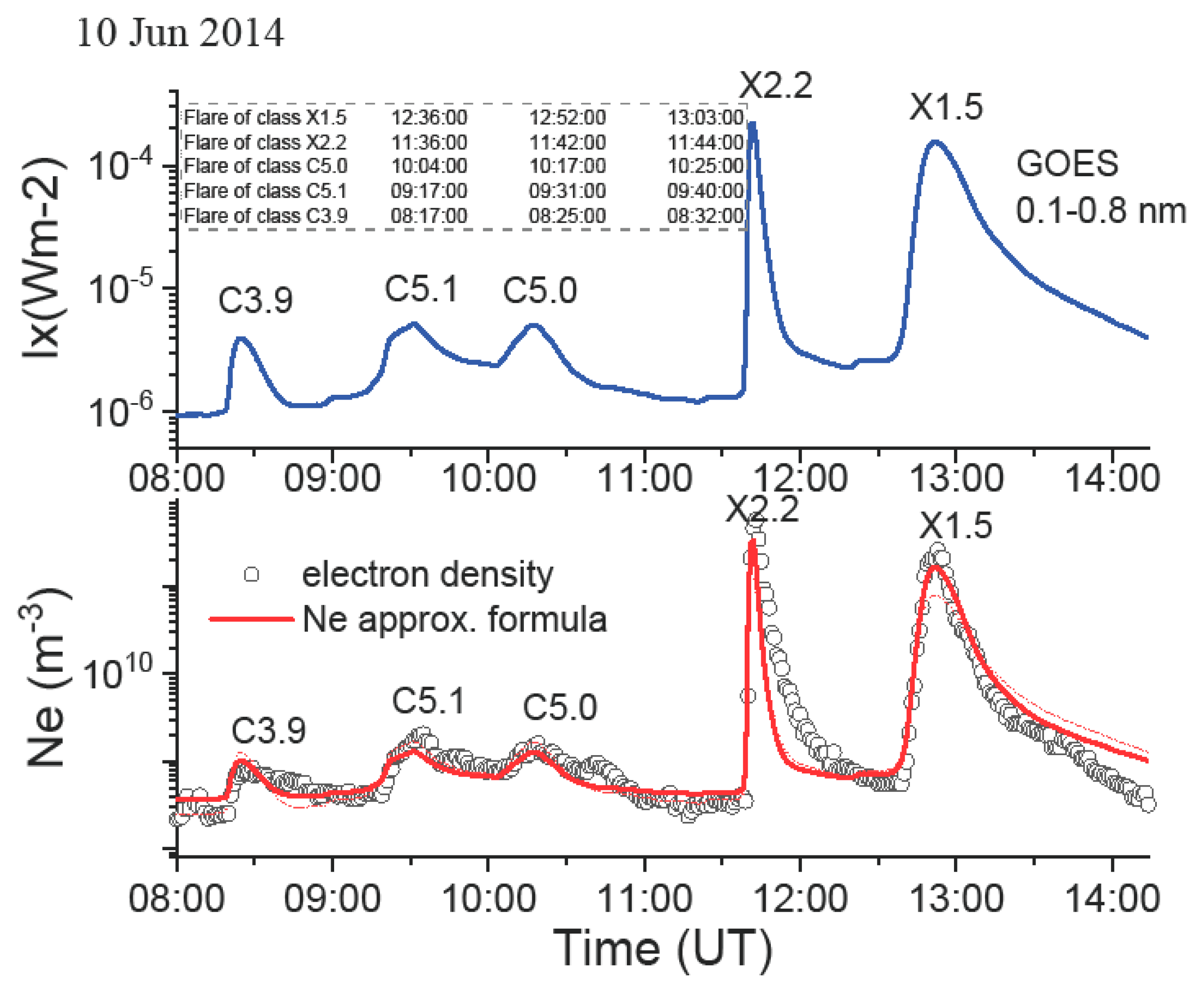
| C3.9 | 08:17 | 08:25 | 08:32 | −1.5 | 0.1 | 3.97 × 10⁻⁶ | 2087 |
| C5.1 | 09:17 | 09:31 | 09:40 | −2 | −7 | 5.18 × 10⁻⁶ | 2087 |
| C5.0 | 10:04 | 10:17 | 10:25 | −0.5 | −9 | 5.06 × 10⁻⁶ | 2087 |
| X2.2 | 11:36 | 11:42 | 11:44 | 7.3 | 32 | 2.22 × 10⁻⁴ | 2087 |
| X1.5 | 12:36 | 12:52 | 13:03 | 7.4 | 15 | 1.55 × 10⁻⁴ | 2087 |
| Height (km) | a1(h) | a2(h) | a3(h) |
|---|---|---|---|
| 50 | 10.3249 | 0.97123 | 0.06168 |
| 55 | 12.94731 | 1.65399 | 0.11341 |
| 60 | 15.56972 | 2.33674 | 0.16513 |
| 65 | 18.19213 | 3.0195 | 0.21686 |
| 70 | 20.81454 | 3.70226 | 0.26858 |
| 75 | 23.43695 | 4.38501 | 0.32031 |
| 80 | 26.05936 | 5.06777 | 0.37203 |
Publisher’s Note: MDPI stays neutral with regard to jurisdictional claims in published maps and institutional affiliations. |
© 2021 by the authors. Licensee MDPI, Basel, Switzerland. This article is an open access article distributed under the terms and conditions of the Creative Commons Attribution (CC BY) license (https://creativecommons.org/licenses/by/4.0/).
Share and Cite
Srećković, V.A.; Šulić, D.M.; Ignjatović, L.; Vujčić, V. Low Ionosphere under Influence of Strong Solar Radiation: Diagnostics and Modeling. Appl. Sci. 2021, 11, 7194. https://doi.org/10.3390/app11167194
Srećković VA, Šulić DM, Ignjatović L, Vujčić V. Low Ionosphere under Influence of Strong Solar Radiation: Diagnostics and Modeling. Applied Sciences. 2021; 11(16):7194. https://doi.org/10.3390/app11167194
Chicago/Turabian StyleSrećković, Vladimir A., Desanka M. Šulić, Ljubinko Ignjatović, and Veljko Vujčić. 2021. "Low Ionosphere under Influence of Strong Solar Radiation: Diagnostics and Modeling" Applied Sciences 11, no. 16: 7194. https://doi.org/10.3390/app11167194
APA StyleSrećković, V. A., Šulić, D. M., Ignjatović, L., & Vujčić, V. (2021). Low Ionosphere under Influence of Strong Solar Radiation: Diagnostics and Modeling. Applied Sciences, 11(16), 7194. https://doi.org/10.3390/app11167194