
Experimental Validation of Non-Marker Simple Image Displacement Measurements for Railway Bridges


Abstract
:1. Introduction
2. Related Contributions
3. Processing and Test Methods
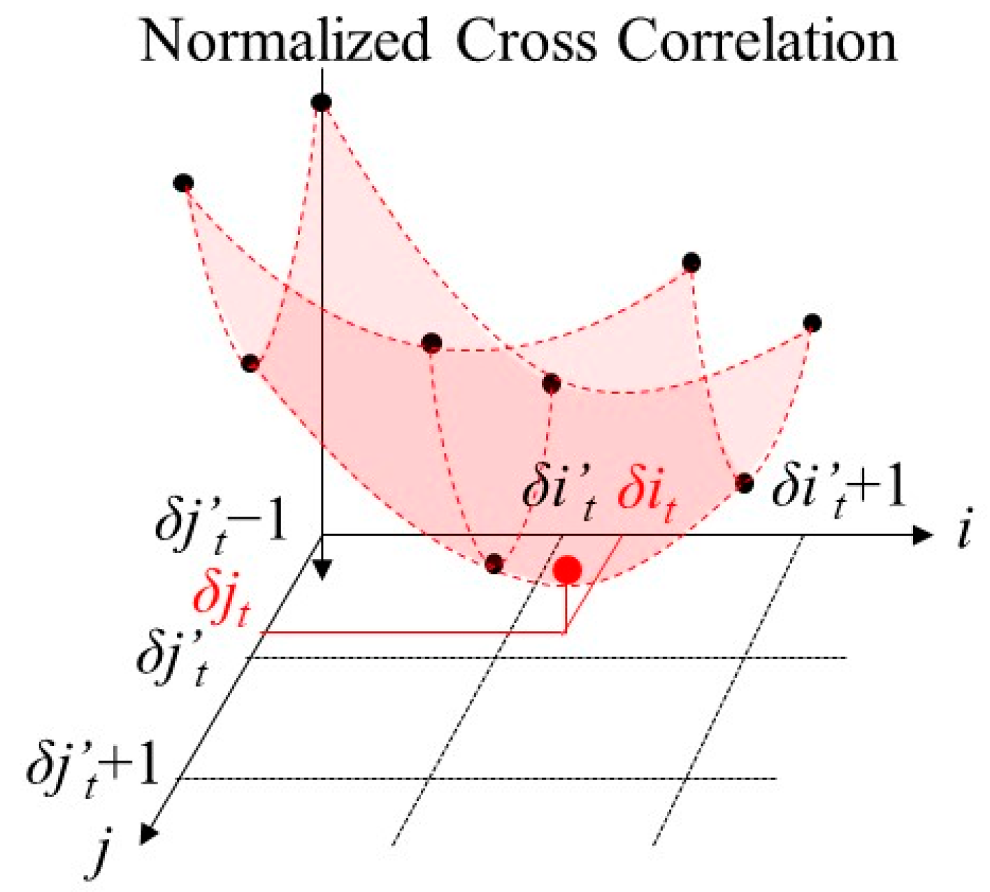
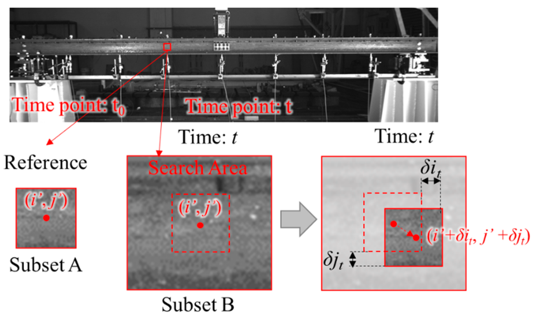
3.1. Image Processing Method
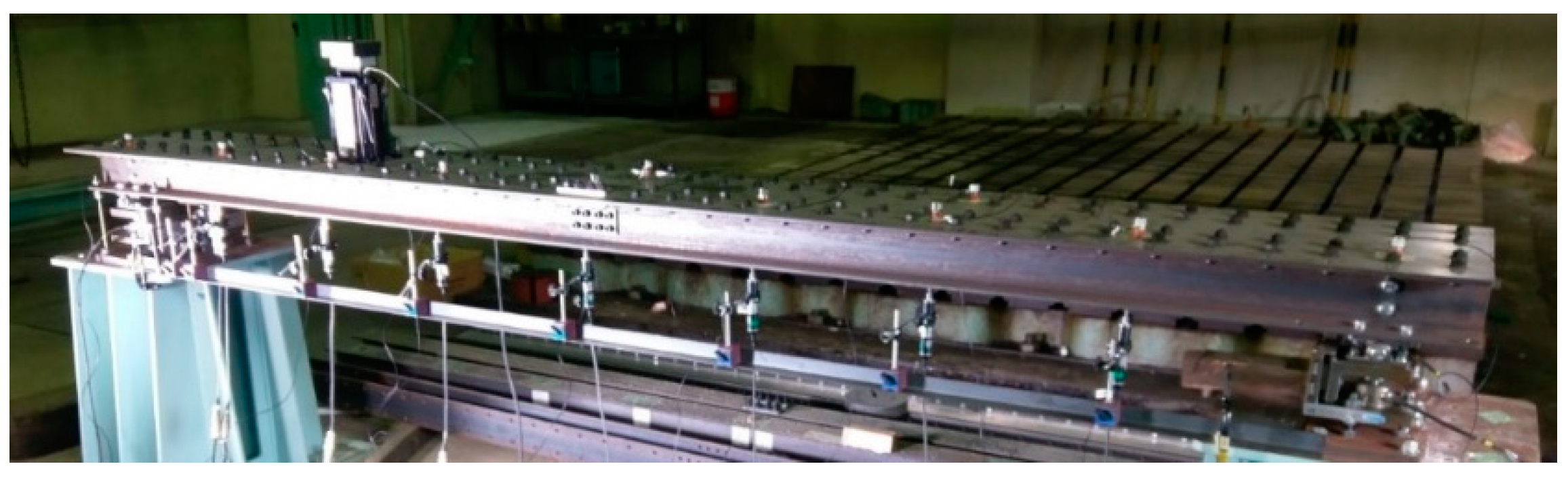
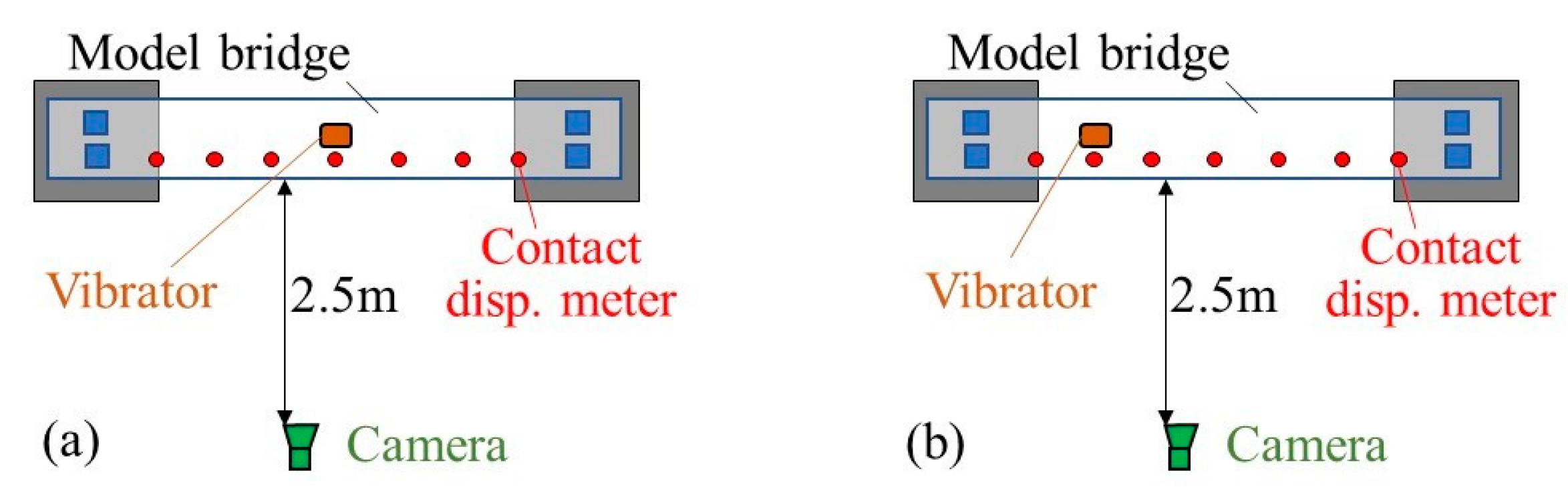
3.2. Model Experiment Method
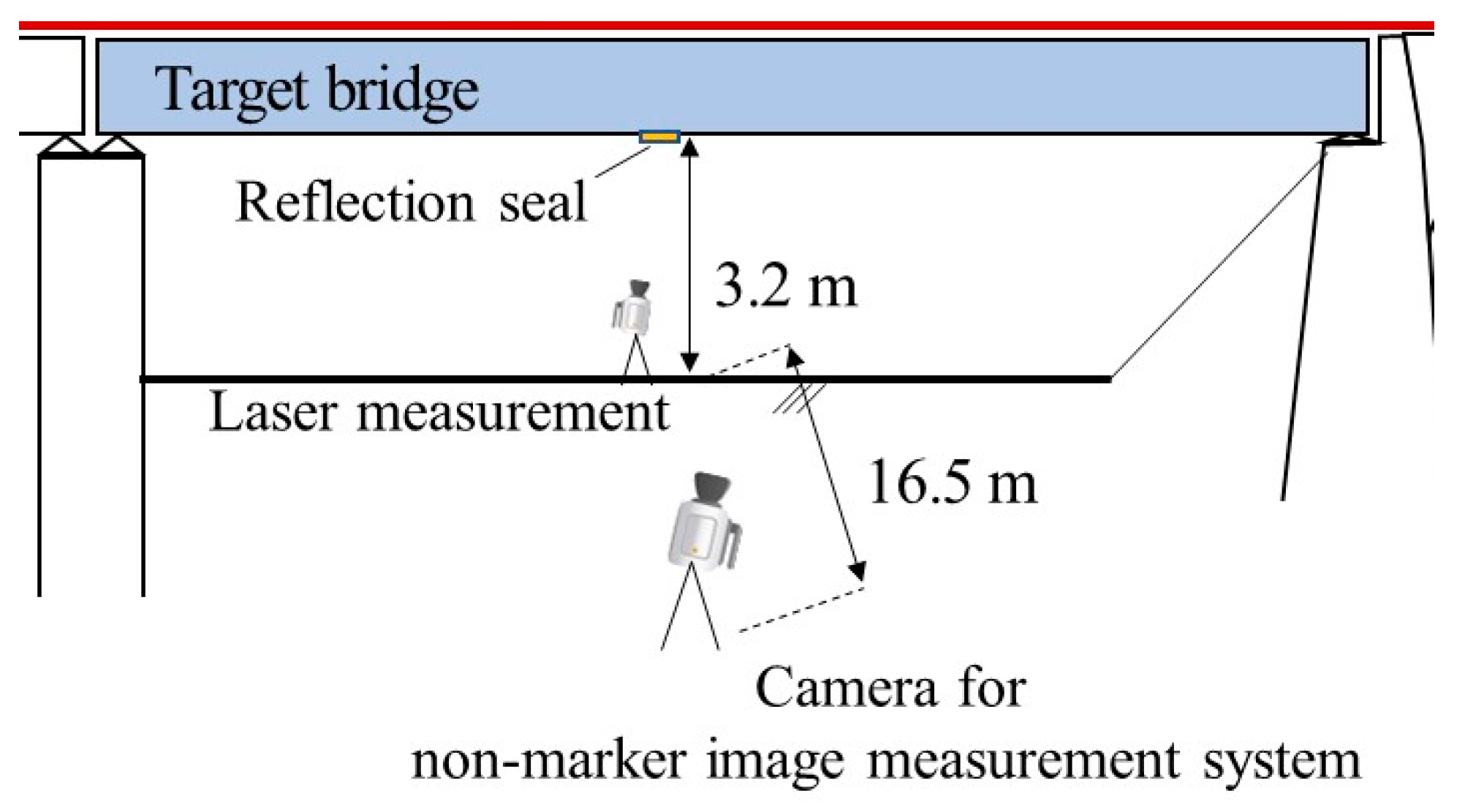
3.3. Field Measurements Method
4. Verification Results by Model Bridge
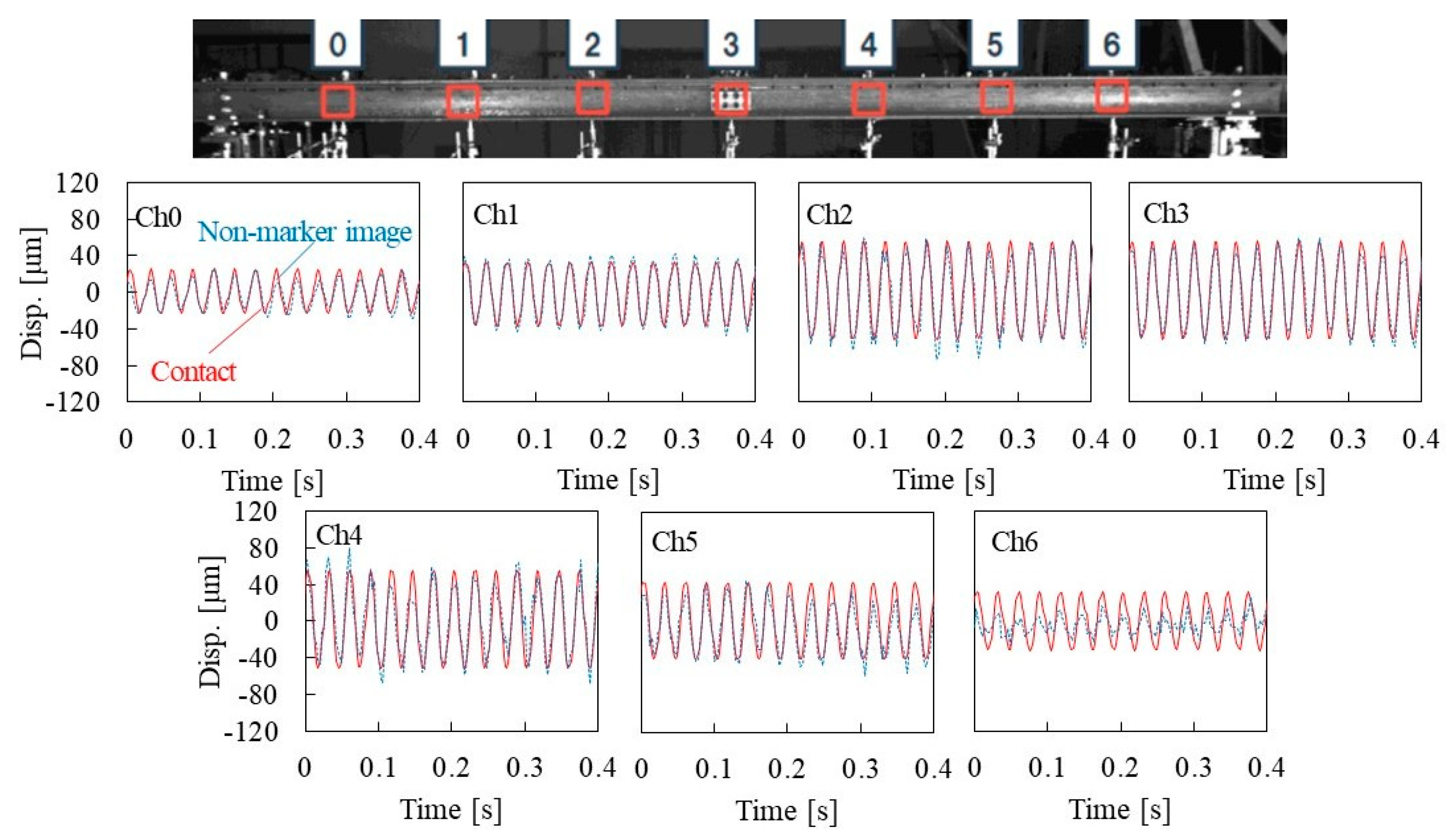
4.1. Measurement Results
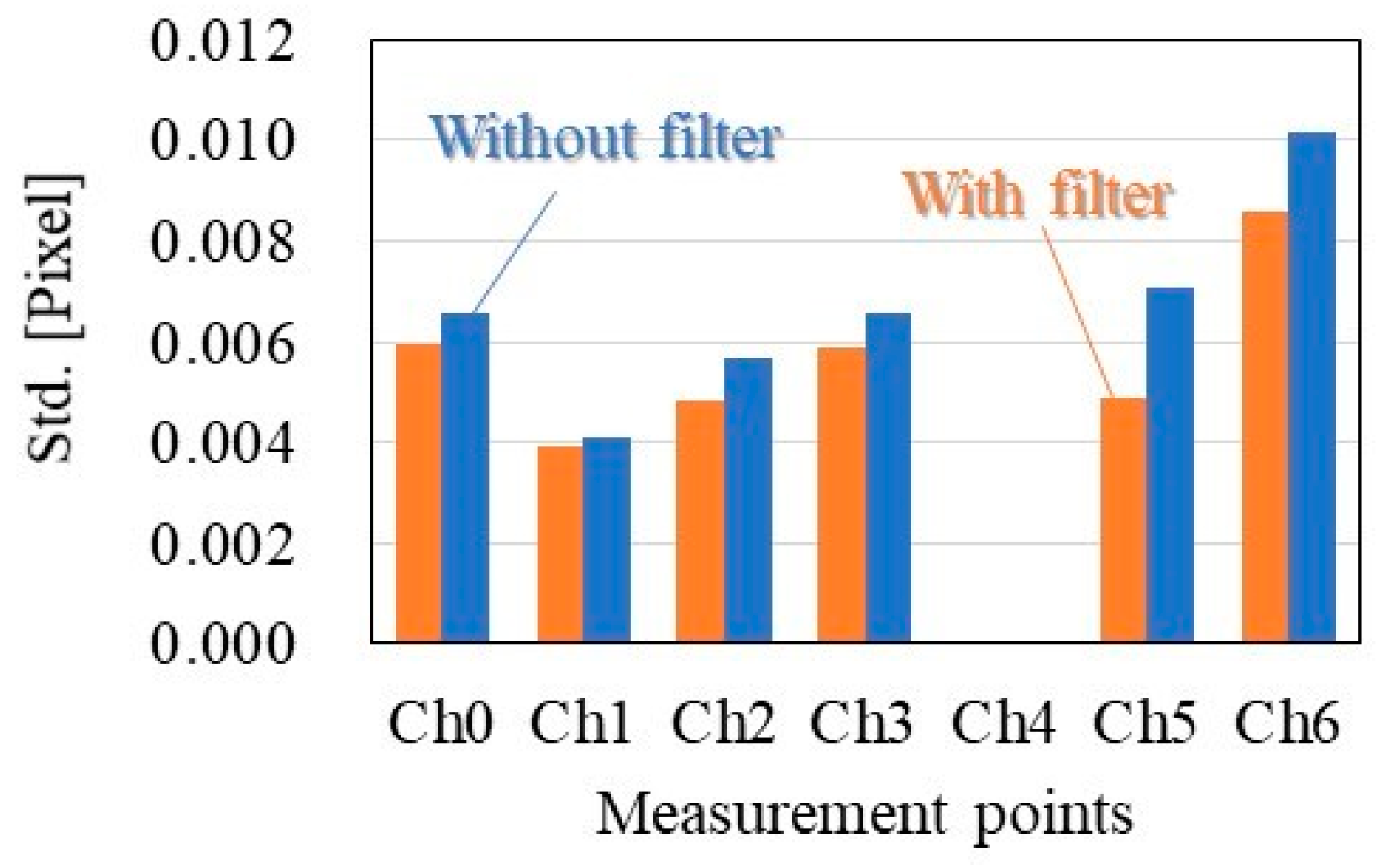
4.2. Measurement Accuracy
4.3. Measurement Results with Minute Amplitude
4.4. Discussion for Practical Application I: Camera Distance
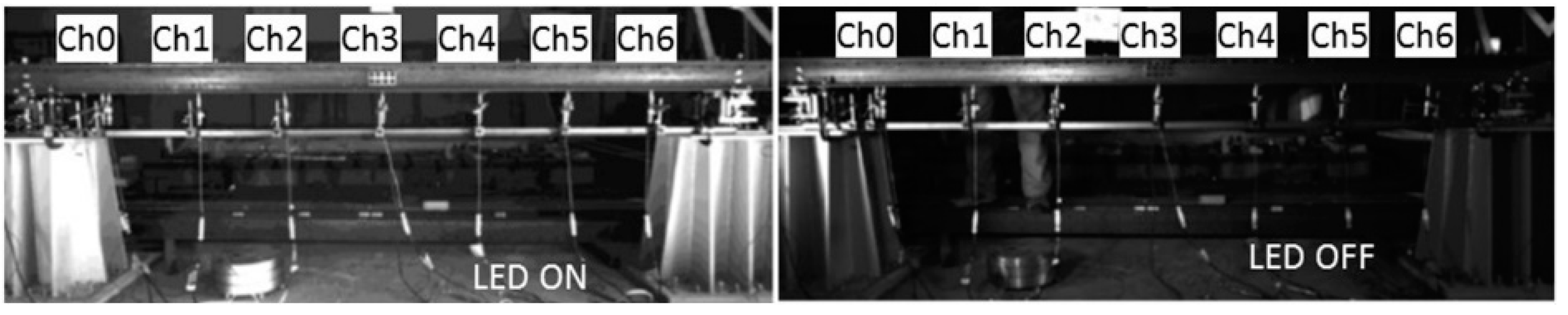
4.5. Discussion for Practical Application II: Effect of Weather (Illuminance)
5. Verification Results of Field Tests
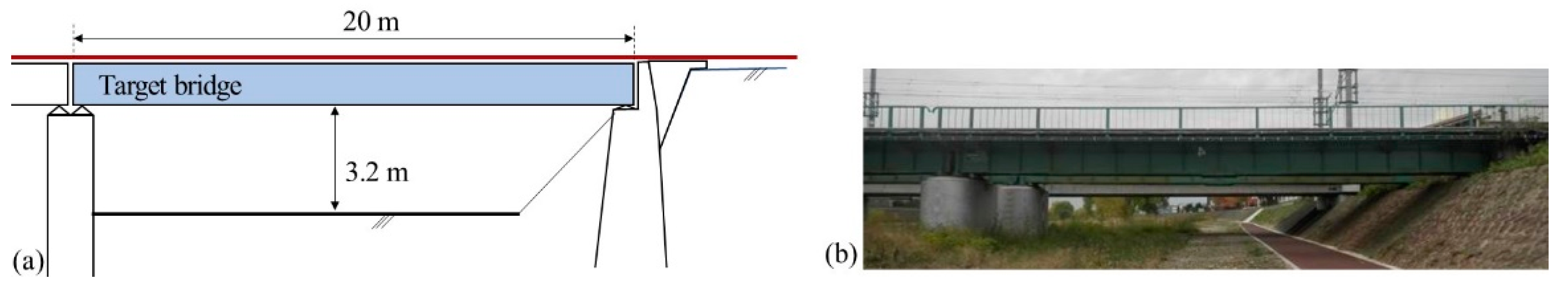
5.1. Measurement Results of Bridge A
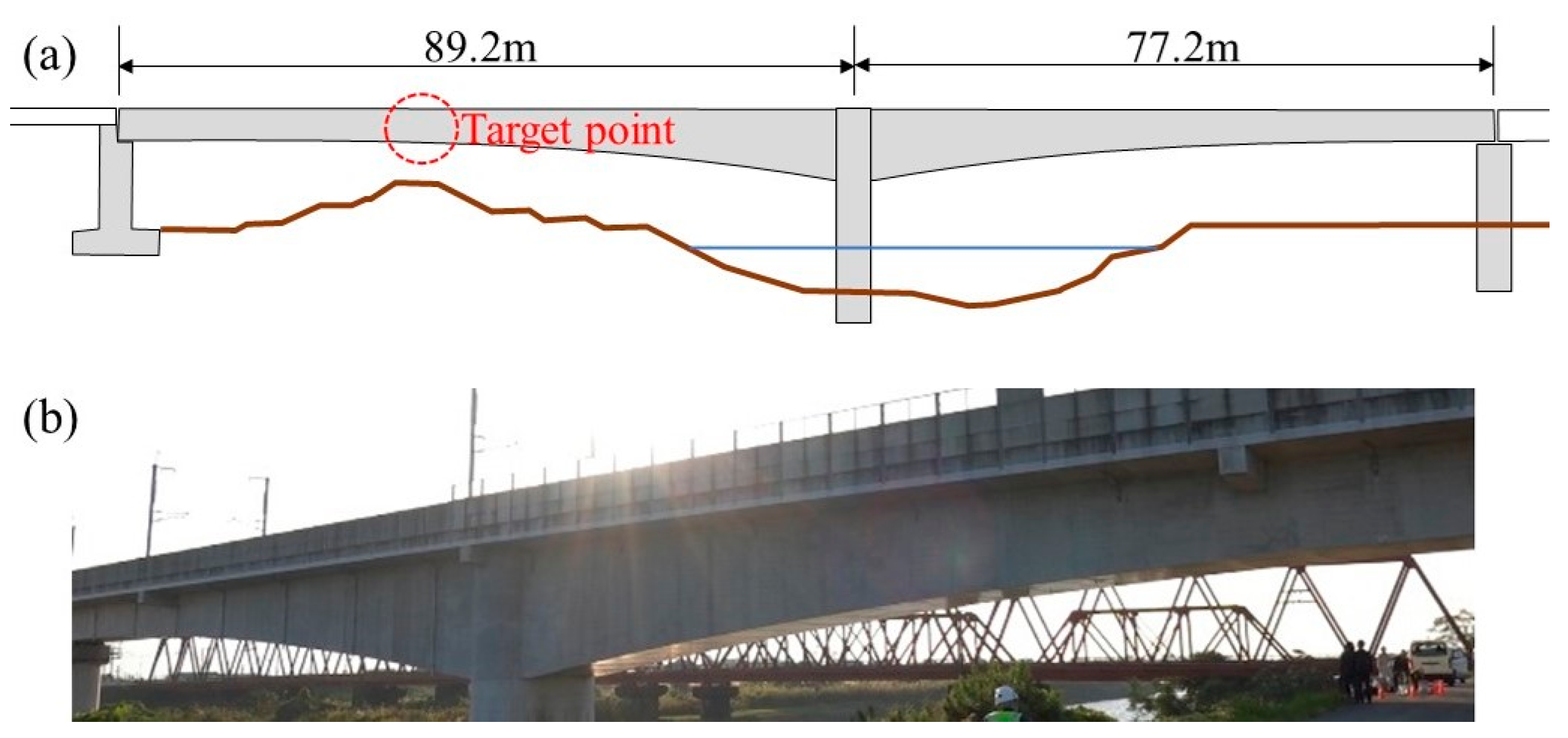
5.2. Measurement Results of Bridge B
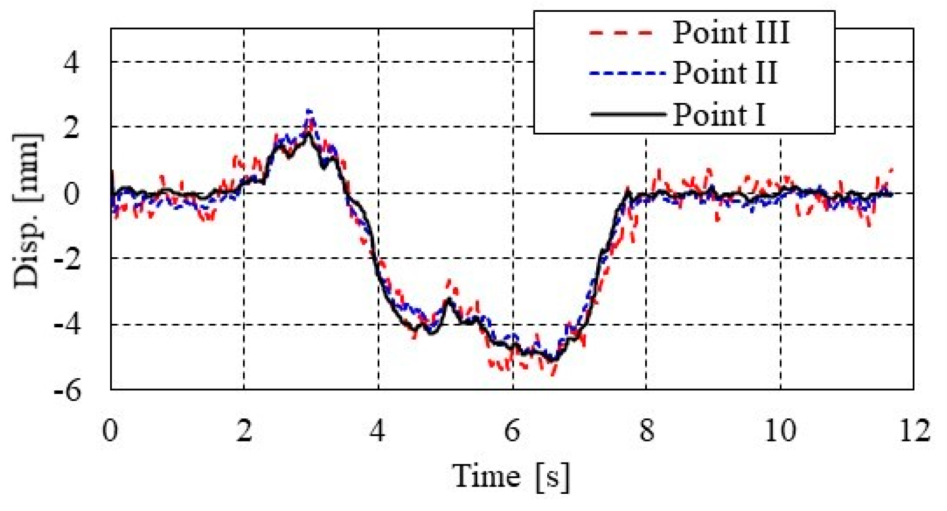
5.3. Discussion of Displacement Measurement of Bridge B (Concrete Bridge)
6. Conclusions
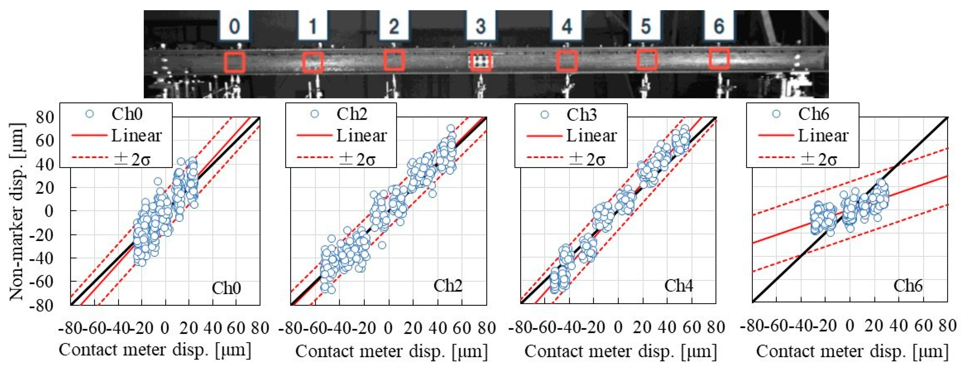
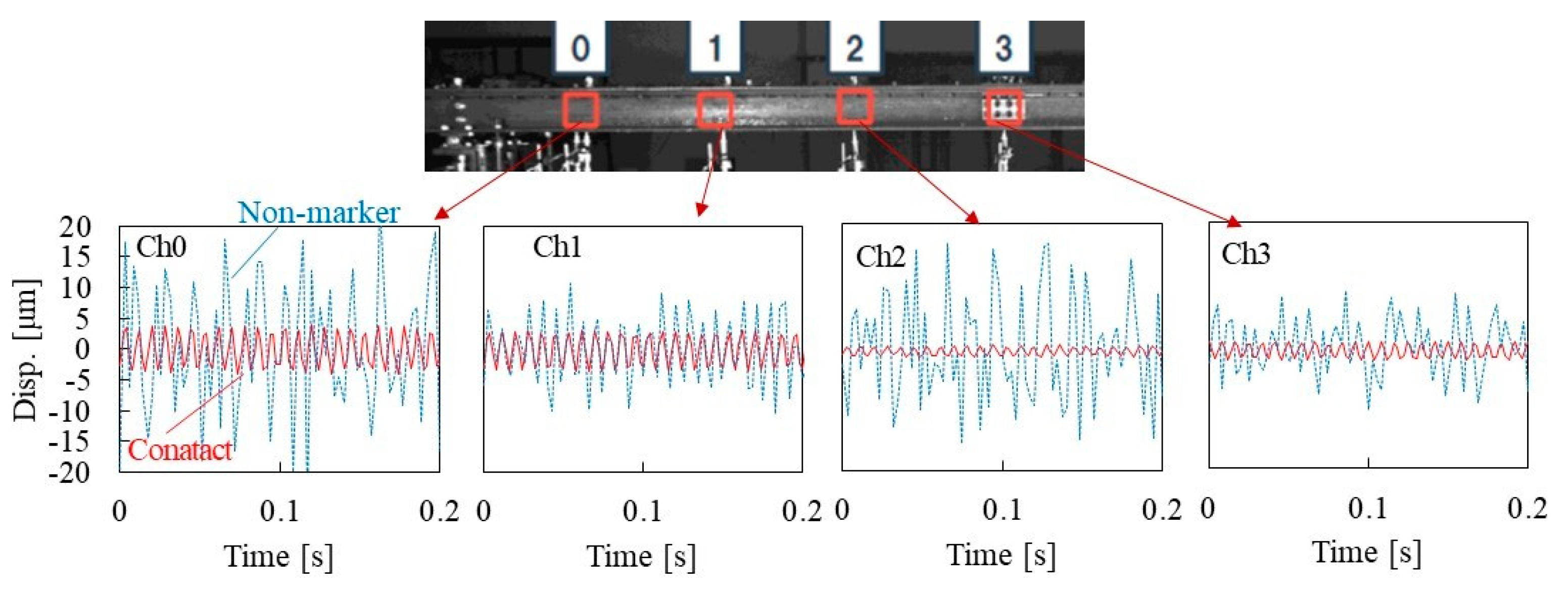
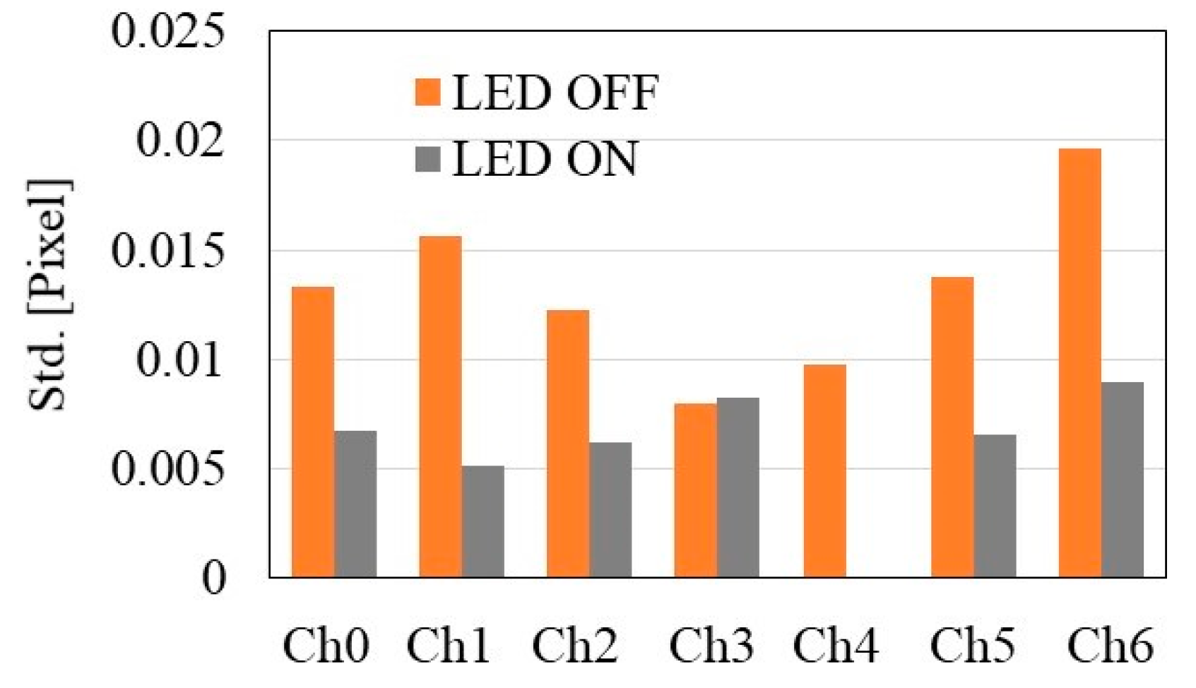
- The multipoint displacement measurement accuracy of non-marker image measurement was verified by exciting a model bridge at seven measurement points and exciting minute displacements with a vertical amplitude of ±25 to 50 μm (±0.017 to 0.035 pixels). Consequently, it was established that displacements greater than 0.03 pixels can be quantified using the non-marker image measurement by avoiding the overexposed areas.
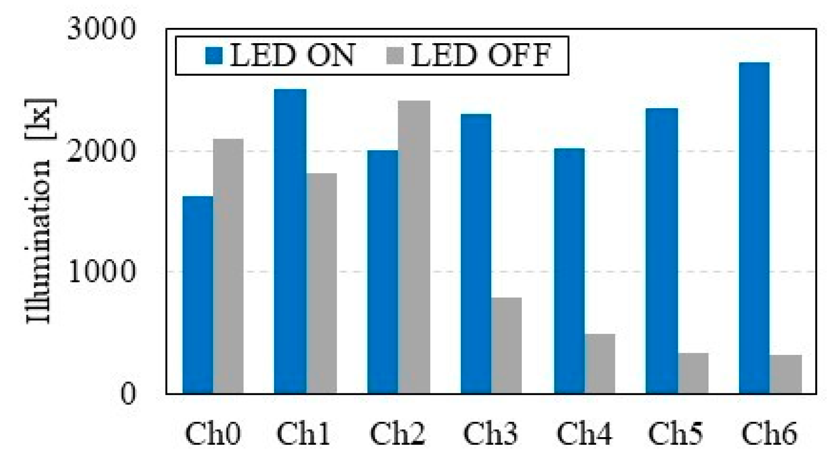
- From the measurement results with varying illuminance, it was estimated that the illuminance required to apply the non-marker image measurement is ~500 lx, and the proposed method can be applied during the daytime.
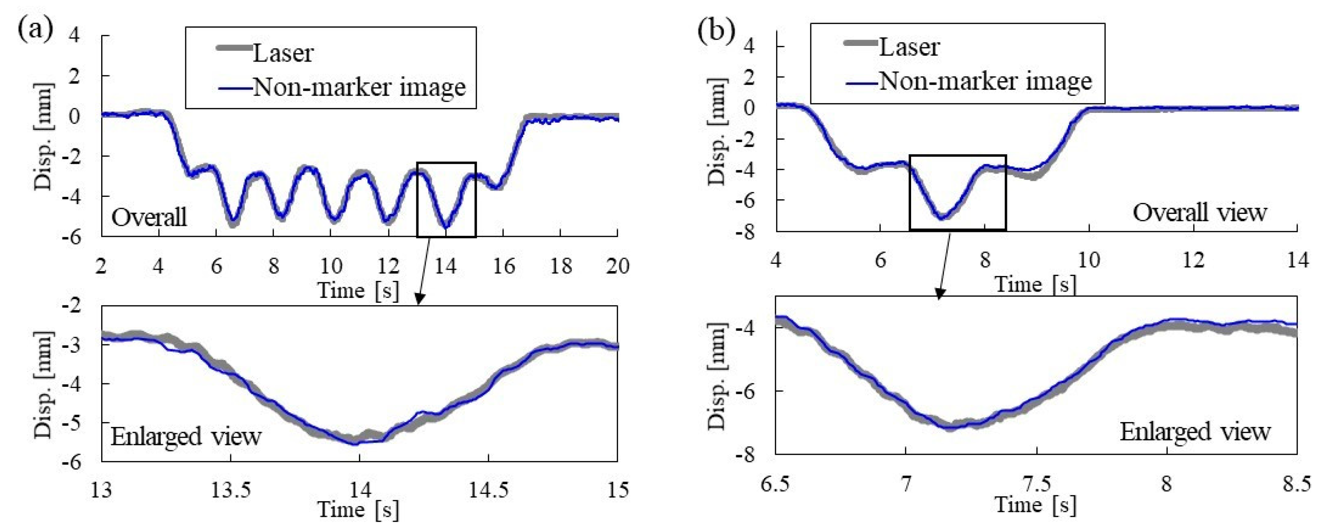
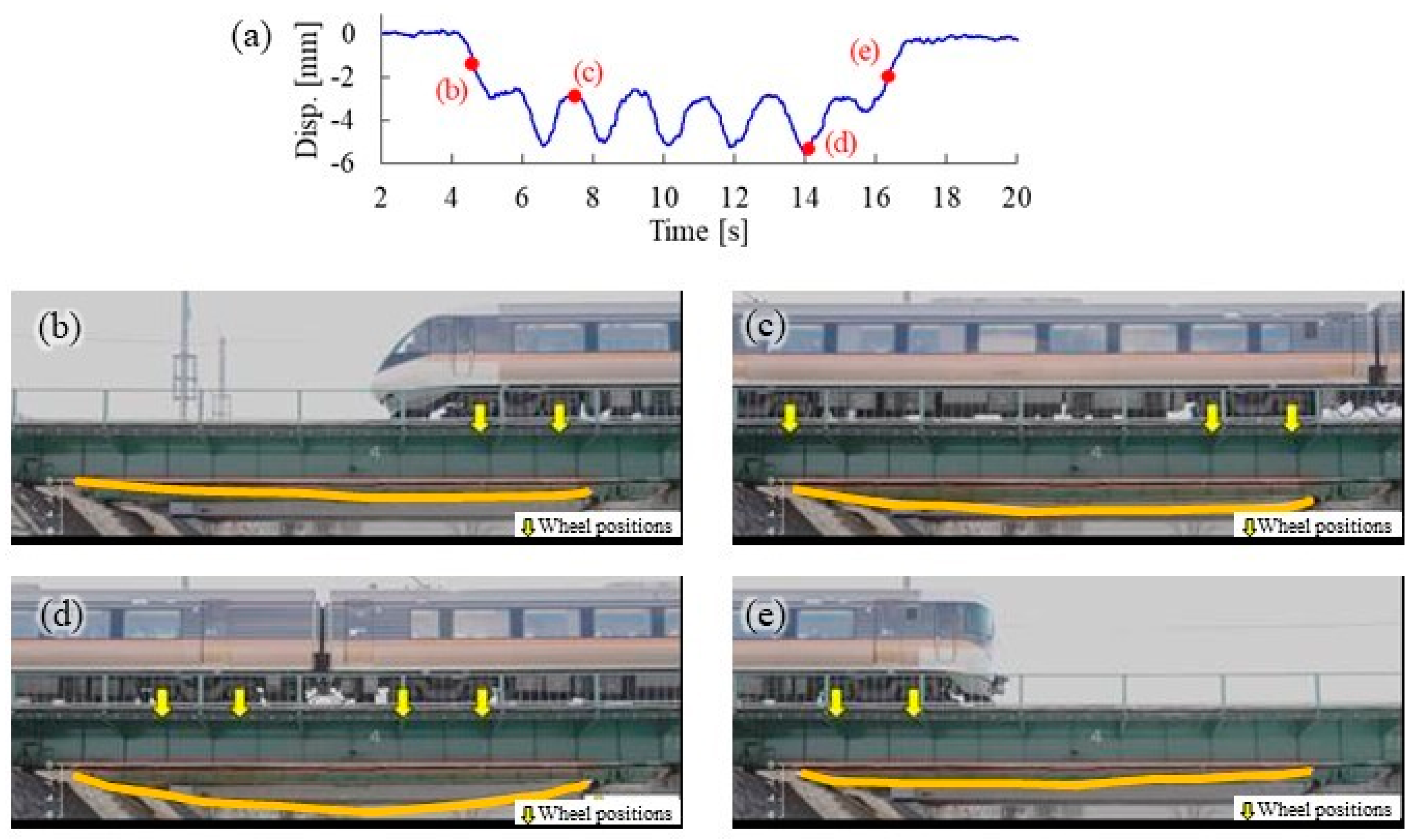
- The displacements during train passages of the steel bridge A (span length 20 m), which had a clear contrast at the image measurement point, were measured using non-marker image measurement and compared with the result of laser measurement. It was confirmed that the non-marker image measurement can be used to estimate the displacement response at the bridge midspan with the same accuracy as that of other measurement approaches.
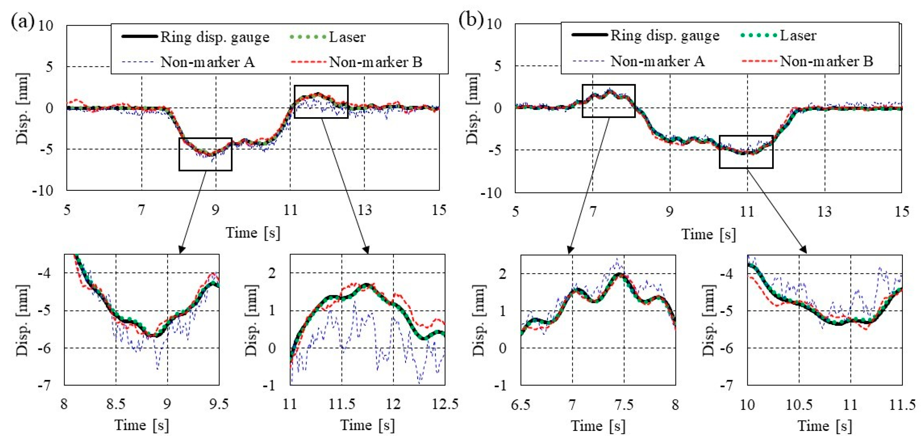
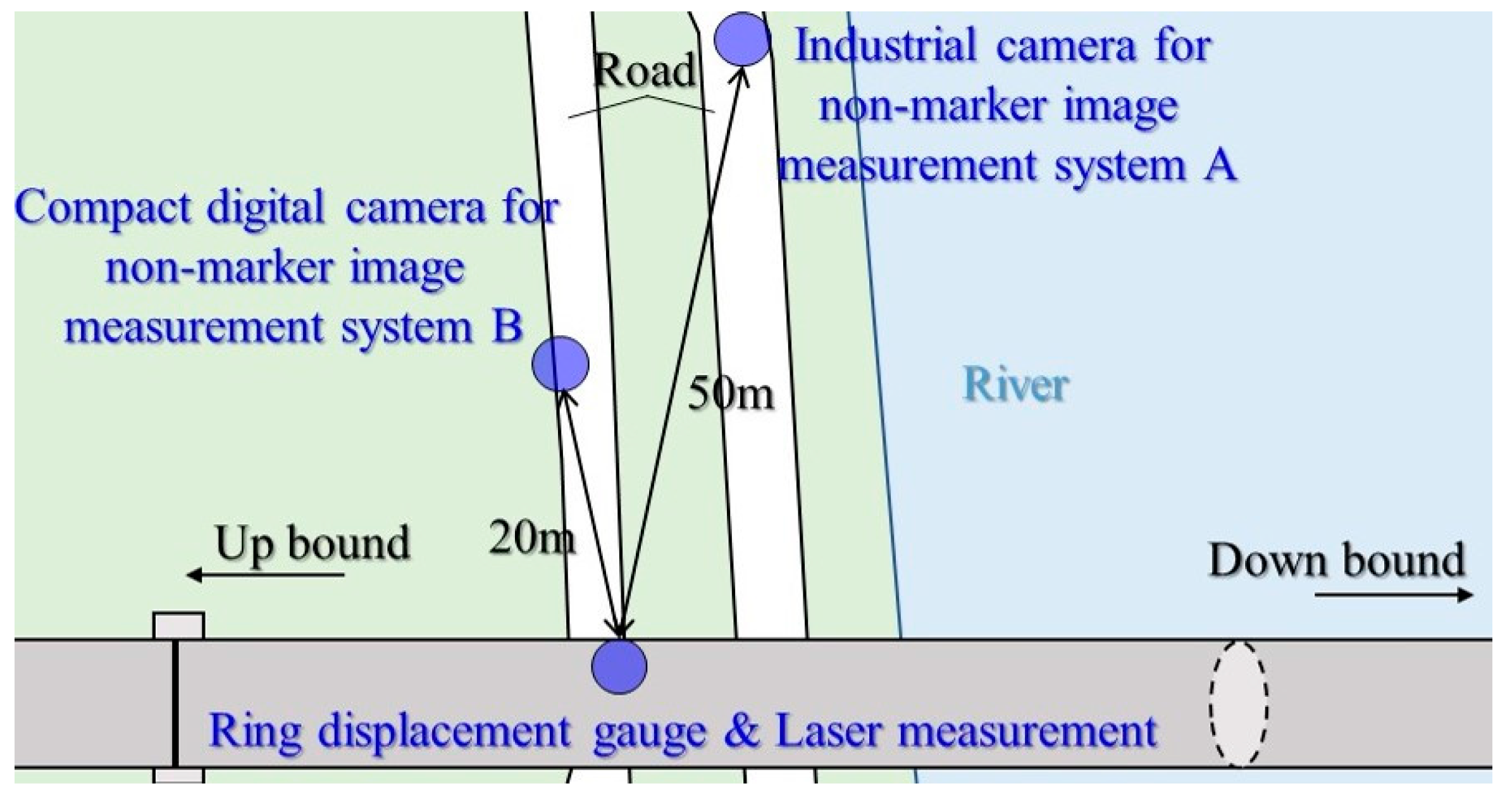
- The displacements during train passages of the high-speed railway bridge B (continuous concrete bridge), which had an unclear contrast, were measured using two types of non-marker image measurement and compared with the results obtained from the ring-type gauge and laser measurement. Consequently, the measurement error of the maximum displacement was ~0.3 mm at a camera distance of ~20 m from the bridge.
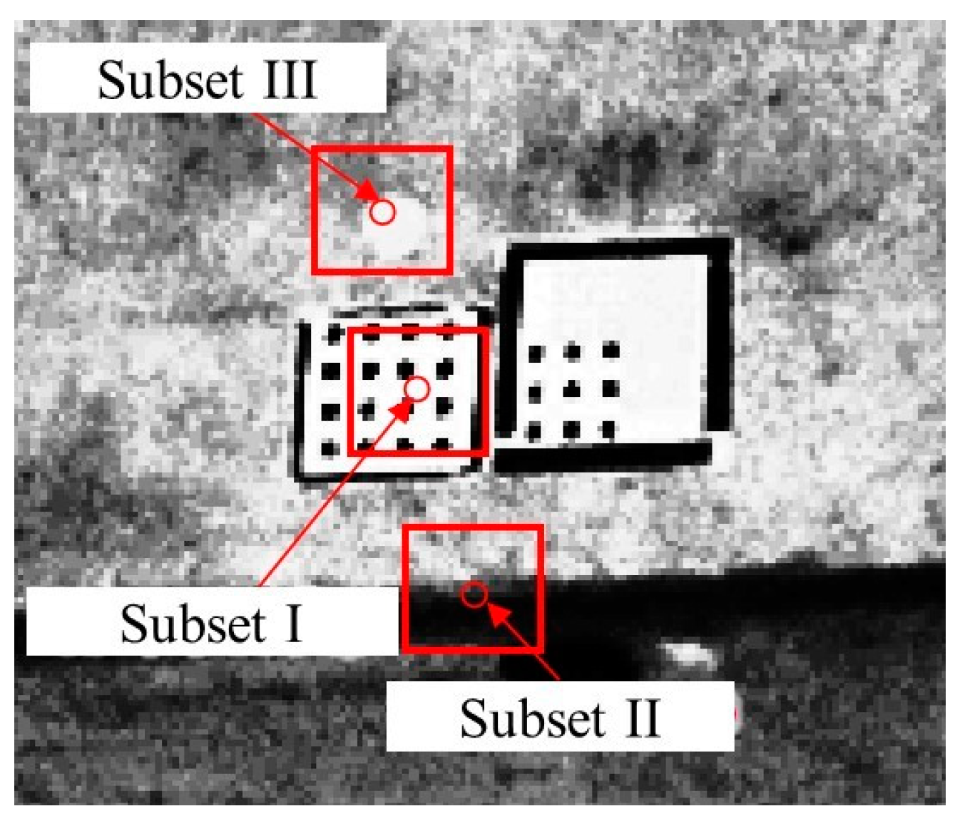
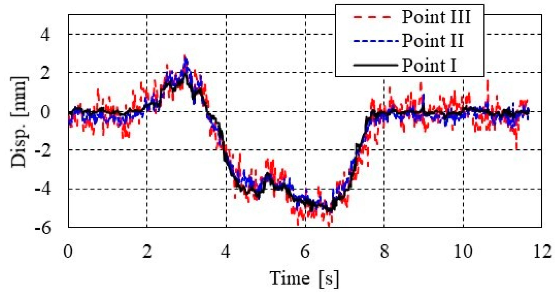
- By examining the error reduction effect of the subset position and moving average processing when the contrast of the image measurement point was not clear, the error was halved by setting the subset on the side of the bottom boundary with a clear texture and using 0.1 s moving average processing.
Author Contributions
Funding
Institutional Review Board Statement
Informed Consent Statement
Acknowledgments
Conflicts of Interest
References
- Matsuoka, K.; Kiyoyuki, K. Vibration Properties of 24 Old Railway Bridges of Same Structure. In IABSE Congress Report; International Association for Bridge and Structural Engineering (IABSE): Zurich, Switzerland, 2012; Volume 18, pp. 1702–1709. [Google Scholar]
- Sofi, A.; Regita, J.J.; Rane, B.; Lau, H.H. Structural health monitoring using wireless smart sensor network—An overview. Mech. Syst. Signal Process. 2022, 163, 108113. [Google Scholar] [CrossRef]
- Qing, X.P.; Beard, S.J.; Ikegami, R.; Chang, F.K.; Boller, C. Encyclopedia of structural health monitoring. In Encyclopedia of Structural Health Monitoring; John Wiley & Sons Ltd.: Hoboken, NJ, USA, 2009. [Google Scholar]
- Fujino, Y.; Siringoringo, D.M. Bridge monitoring in Japan: The needs and strategies. Struct. Infrastruct. Eng. 2011, 7, 597–611. [Google Scholar] [CrossRef]
- Sogabe, M.; Furukawa, A.; Shimomura, T.; Iida, T.; Matsumoto, N.; Wakui, H. Deflection limits of structures for train speed-up. Q. Rep. RTRI 2005, 46, 130–136. [Google Scholar] [CrossRef] [Green Version]
- Uehan, F. Development of the U-Doppler non-contact vibration measuring system for diagnosis of railway structures. Q. Rep. RTRI 2008, 49, 178–183. [Google Scholar] [CrossRef] [Green Version]
- Acikgoz, S.; DeJong, M.J.; Soga, K. Sensing dynamic displacements in masonry rail bridges using 2D digital image correlation. Struct. Control Health Monit. 2018, 25, e2187. [Google Scholar] [CrossRef] [Green Version]
- Malesa, M.; Szczepanek, D.; Kujawińska, M.; Świercz, A.; Kołakowski, P. Monitoring of Civil Engineering Structures using Digital Image Correlation technique. EPJ Web Conf. 2010, 6, 31014. [Google Scholar] [CrossRef] [Green Version]
- Matsuoka, K.; Uehan, F.; Kusaka, H.; Imagawa, T.; Noda, A. Accuracy verification of girder deflection shape measurement by non-target optical measurement and its applicability. J. Jpn. Soc. Civ. Eng. 2018, 74, I_715–I_726. [Google Scholar] [CrossRef]
- Lee, J.J.; Shinozuka, M. A vision-based system for remote sensing of bridge displacement. NDT E Int. 2006, 39, 425–431. [Google Scholar]
- Choi, H.S.; Cheung, J.H.; Kim, S.H.; Ahn, J.H. Structural dynamic displacement vision system using digital image processing. NDT E Int. 2011, 44, 597–608. [Google Scholar]
- Ribeiro, D.; Calçada, R.; Ferreira, J.; Martins, T. Non-contact measurement of the dynamic displacement of railway bridges using an advanced video-based system. Eng. Struct. 2014, 75, 164–180. [Google Scholar] [CrossRef]
- Cigada, A.; Mazzoleni, P.; Zappa, E. Vibration monitoring of multiple bridge points by means of a unique vision-based measuring system. Exp. Mech. 2014, 54, 255–271. [Google Scholar]
- Feng, D.; Feng, M.Q.; Ozer, E.; Fukuda, Y. A vision-based sensor for noncontact structural displacement measurement. Sensors 2015, 15, 16557–16575. [Google Scholar] [CrossRef] [PubMed]
- Fukuda, Y.; Feng, M.Q.; Narita, Y.; Kaneko, S.I.; Tanaka, T. Vision-based displacement sensor for monitoring dynamic response using robust object search algorithm. IEEE Sens. J. 2013, 13, 4725–4732. [Google Scholar] [CrossRef] [Green Version]
- Feng, M.Q.; Fukuda, Y.; Feng, D.; Mizuta, M. Nontarget vision sensor for remote measurement of bridge dynamic response. J. Bridge Eng. 2015, 20, 04015023. [Google Scholar] [CrossRef]
- Pan, B.; Tian, L.; Song, X. Real-time, non-contact and targetless measurement of vertical deflection of bridges using off-axis digital image correlation. NDT E Int. 2016, 79, 73–80. [Google Scholar] [CrossRef]
- Feng, D.; Feng, M.Q. Computer vision for SHM of civil infrastructure: From dynamic response measurement to damage detection—A review. Eng. Struct. 2018, 156, 105–117. [Google Scholar] [CrossRef]
- Xu, Y.; Brownjohn, J.M. Review of machine-vision based methodologies for displacement measurement in civil structures. J. Civ. Struct. Health Monit. 2018, 8, 91–110. [Google Scholar] [CrossRef] [Green Version]
- Ribeiro, D.; Santos, R.; Cabral, R.; Saramago, G.; Montenegro, P.; Carvalho, H.; Correia, J.; Calçada, R. Non-contact structural displacement measurement using unmanned aerial vehicles and video-based systems. Mech. Syst. Signal Proces. 2021, 160, 107869. [Google Scholar] [CrossRef]
- Yoneyama, S.; Kitagawa, A.; Iwata, S.; Tani, K.; Kitamura, K.; Kikuta, H. Noncontact deflection distribution measurement of bridges using digital image correlation. Hihakai Kensa (J. NDI) 2006, 55, 119–125. [Google Scholar]
- Shimizu, M.; Okutomi, M. Precise subpixel estimation on area-based matching. Syst. Comput. Jpn. 2002, 33, 1–10. [Google Scholar] [CrossRef]
- Keren, D.; Peleg, S.; Brada, R. Image sequence enhancement using sub-pixel displacements. CVPR 1988, 88, 5–9. [Google Scholar]
- Wu, S.; Ren, J.; Chen, Z.; Jin, W.; Liu, X.; Li, H.; Pan, H.; Guo, W. Influence of reconstruction scale, spatial resolution and pixel spatial relationships on the sub-pixel mapping accuracy of a double-calculated spatial attraction model. Remote Sens. Environ. 2018, 210, 345–361. [Google Scholar] [CrossRef]
- Shimizu, M.; Okutomi, M. Significance and attributes of subpixel estimation on area-based matching. Syst. Comput. Jpn. 2003, 34, 1–10. [Google Scholar] [CrossRef]
- Matsuoka, K.; Collina, A.; Somaschini, C.; Sogabe, M. Influence of local deck vibrations on the evaluation of the maximum acceleration of a steel-concrete composite bridge for a high-speed railway. Eng. Struct. 2019, 200, 109736. [Google Scholar] [CrossRef]
- Matsuoka, K.; Tanaka, H.; Kawasaki, K.; Somaschini, C.; Collina, A. Drive-by methodology to identify resonant bridges using track irregularity measured by high-speed trains. Mech. Syst. Signal Process. 2021, 158, 107667. [Google Scholar] [CrossRef]
- Matsuoka, K.; Tokunaga, M.; Kaito, K. Bayesian estimation of instantaneous frequency reduction on cracked concrete railway bridges under high-speed train passage. Mech. Syst. Signal Process. 2021, 161, 107944. [Google Scholar] [CrossRef]
- Koyomi Handbook Editorial Board. Koyomi Handbook; Osaka Science Museum: Osaka, Japan, 2020. [Google Scholar]
- Matsuoka, K.; Kawasaki, K.; Tanaka, H.; Tsunemoto, M. On-board resonant bridge detection method using carbody vertical accelerations of a high-speed train. J. Jpn. Soc. Civ. Eng. 2021, 77, 146–164. [Google Scholar]
- Matsuoka, K.; Munemasa, T.; Tsunemoto, M.; Ikura, K. A study of pole vibration built on the railway bridges under train passage. In Proceedings of the Transportation and Logistics Conference, Tokyo, Japan, 7 December 2018; Volume 27, p. 1513. [Google Scholar]


| Specifications | Values |
|---|---|
| Bridge length | 3048 mm |
| Bridge span | 2800 mm |
| Mass (without noise barrier) | 230 kg/197 kg |
| Girder | 2 × H-100 |
| Deck | 3048 × 400 × 9 mm |
| Calculated frequency | 37 Hz |
| Equipment | Product Models | Companies | Specifications |
|---|---|---|---|
| Contact displacement gauge | CFP-10 | Tokyo Sokki (Shinagawa, Tokyo, Japan) | Range: 10 mm Output:5 mV/V Sensitivity: 0.001 ε/mm |
| Data recording | Ni cDAQ-9172 | National Instruments Japan (Minato, Tokyo, Japan) | Sampling rate: 2000 Hz |
| Ni9220 | |||
| LabVIEW | |||
| Camera | Flare 4M180-MCX | IO industries (Hamamatsu, Shizuoka, Japan) | Resolution: 2048 × 800 pixel |
| Recorder | DVR Express CORE2 | IO industries (Hamamatsu, Shizuoka, Japan) | Sampling rate: 350 Hz |
| Lens | LM8XC2 | Kowa Company. Ltd. (Nagoya, Aichi, Japan) | Focal length: 8.5 mm |
| Types | Simply Supported Bridge |
|---|---|
| Maximum speed | 100 km/h |
| Span length | 20 m |
| Girder height | 1.4 m |
| Girder type | I type steel girder × 2 |
| Track | Wooden sleeper single track (without slab) |
| Moment of inertia of area | 0.062 m4 |
| Frequency | 13.03 Hz |
| Types | Simply Supported Bridge |
|---|---|
| Maximum speed | 260 km/h |
| Span length | 89.2 m + 77.2 m |
| Girder height | 1.5–3.2 m |
| Girder type | Concrete box |
| Track | Ballastless double track |
| Measurement Methods | Measurement Principles | Specifications |
|---|---|---|
| Self-vibration correction laser Doppler velocimeter (Laser measurement)  | Displacement is calculated by integrating the vibration velocity measured with a laser Doppler velocimeter | Non-contact With reflective marker Sampling rate: 500 Hz |
Non-marker image measurement | Displacement is calculated from the image by DIC (Section 3.1) | Resolution: 1920 × 600 pixel Sampling rate: 120 fps Camera: GS3-U3-23S6M-C Lens: LM8XC2 |
| Measurement Methods | Measurement Principles | Specifications |
|---|---|---|
Ring type gauge  Wire fixing jig, gauge | Displacement is converted from the strain of the ring gauge installed on a piano wire connecting the girder to the ground. | Sampling rate: 1000 Hz |
| Self-vibration correction laser Doppler velocimeter (laser measurement)  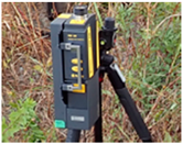 Reflective marker, Doppler meter | Displacement is calculated by integrating the vibration velocity measured with a laser Doppler velocimeter | Non-contact With reflective marker Sampling rate: 500 Hz Measurement distance: 0.1–100 m |
Non-marker image measurement A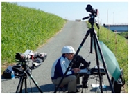 PC-controlled industrial camera | Displacement is calculated from images by DIC (Section 3.1) | Resolution: 4096 × 2160 pixels Camera: Flare 4M180-MCX Sampling rate: 200 fps Lens: wide-angle or standard |
Non-marker image measurement B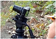 Compact digital camera | Displacement is calculated from images by DIC (Section 3.1) | Resolution: 2048 × 1088 pixel Camera: DSC-RX1004M Sampling rate: 60 Hz |
| Bridge Spans | Bridge Number | Bridge Spans | Bridge Number |
|---|---|---|---|
| Less than 10 m | 4 | 30–40 m | 66 |
| 10–20 m | 13 | 40–50 m | 54 |
| 20–30 m | 44 | Over 50 m | 65 |
| Situation | Time | Illuminance (klx) | Applicability |
|---|---|---|---|
| Outdoor/Sunny | Noon | 100 | ○ |
| 10 AM | 65 | ○ | |
| 3 PM | 35 | ○ | |
| 1 h before sunset | 1 | ○ | |
| Outdoor/Cloudy | Noon | 32 | ○ |
| 10 AM | 25 | ○ | |
| 1 h after sunrise | 2 | ○ | |
| Sunrise/sunset | 0.3 | × | |
| Under the street light | Night | 0.05–0.1 | × |
| Moonlight | Night | 0.0005–0.001 | × |
| Methods | Tests | Maximum Displacements (mm) | Errors (%) |
|---|---|---|---|
| Laser measurement | Six-car train | 5.47 | - |
| non-marker image measurement | 5.64 | 3.1 | |
| Laser measurement | Two-car train | 7.16 | - |
| non-marker image measurement | 7.06 | 1.4 |
| Subset Position | I | II (Reference) | III |
|---|---|---|---|
| Contrasts | high | - | low |
| 2σ values | 0.23 mm | 0.46 mm | 1.16 mm |
| Variations to the reference II | 49% | 100% | 252% |
| Smoothing (0.1 s moving average) | 0.18 mm | 0.27 mm | 0.79 mm |
Publisher’s Note: MDPI stays neutral with regard to jurisdictional claims in published maps and institutional affiliations. |
© 2021 by the authors. Licensee MDPI, Basel, Switzerland. This article is an open access article distributed under the terms and conditions of the Creative Commons Attribution (CC BY) license (https://creativecommons.org/licenses/by/4.0/).
Share and Cite
Matsuoka, K.; Uehan, F.; Kusaka, H.; Tomonaga, H. Experimental Validation of Non-Marker Simple Image Displacement Measurements for Railway Bridges. Appl. Sci. 2021, 11, 7032. https://doi.org/10.3390/app11157032
Matsuoka K, Uehan F, Kusaka H, Tomonaga H. Experimental Validation of Non-Marker Simple Image Displacement Measurements for Railway Bridges. Applied Sciences. 2021; 11(15):7032. https://doi.org/10.3390/app11157032
Chicago/Turabian StyleMatsuoka, Kodai, Fumiaki Uehan, Hiroya Kusaka, and Hikaru Tomonaga. 2021. "Experimental Validation of Non-Marker Simple Image Displacement Measurements for Railway Bridges" Applied Sciences 11, no. 15: 7032. https://doi.org/10.3390/app11157032
APA StyleMatsuoka, K., Uehan, F., Kusaka, H., & Tomonaga, H. (2021). Experimental Validation of Non-Marker Simple Image Displacement Measurements for Railway Bridges. Applied Sciences, 11(15), 7032. https://doi.org/10.3390/app11157032