Optimization of Relief Well Design Using Artificial Neural Network during Geological CO₂ Storage in Pohang Basin, South Korea

Abstract

This study aims at the development of an artificial neural network (ANN) model to optimize relief well design in Pohang Basin, South Korea. Relief well design in carbon capture and geological storage (CCS) requires complex processes and excessive iterative procedures to obtain optimal operating parameters, such as CO₂ injection rate, water production rate, distance between the wells, and pressure at the wells. To generate training and testing datasets for ANN model development, optimization processes for a relief well with various injection scenarios were performed. Training and testing were conducted, where the best iteration and regression were considered based on the calculated coefficient of determination (R²) and root mean square error (RMSE) values. According to validation with a 20-year injection scenario, which was not included in the training datasets, the model showed great performance with R² values of 0.96 or higher for all the output parameters. In addition, the RMSE values for the BHP and the trapping mechanisms were lower than 0.04. Moreover, the location of the relief well was reliably predicted with a distance difference of only 20.1 m. The ANN model can be robust tool to optimize relief well design without a time-consuming reservoir simulations.

1. Introduction

Carbon capture and geological storage (CCS) has been considered a promising method of greenhouse gas reduction [1]. To develop cost-effective and stable CCS technology, experimental studies have been performed to identify potential rock property alterations due to injected CO₂ with experimental approaches, such as core analysis and X-ray diffraction (XRD) [2,3]. There are related numerical studies focusing on CO₂ plume migration and stability analysis to analyze potential CO₂ migration pathways and the maximum sustainable injection pressure during geological storage of CO₂ [4,5]. In addition, a few studies have also been performed to monitor field-scale behavior, such as seabed deformation [6,7]. In 2019, globally, there were 51 field-scale CCS facilities under operation, construction, or under serious consideration [8].

According to the Paris Agreement in 2015, South Korea, which is the eighth largest CO₂-emitting country in the world, needs to reduce its greenhouse gas emission by 37% of the business-as-usual (BAU) value by 2030 (850.6 MtCO₂e), aiming at 536 MtCO₂e [9]. In an attempt to achieve the goal, Korea’s national R&D programs have been focusing on practical designs of CCS [10]. Although CCS is generally aimed at depleted hydrocarbon reservoirs, saline aquifers, and salt caverns, South Korea is primarily targeting deep saline aquifers as the country has quite restricted geological alternatives [11,12,13].

For the successful application of a CCS project, the first step is to find a secured geological structure with sufficient storage capacity and CO₂ injectivity [14], which strongly depend on reservoir properties, such as porosity, permeability, and geological boundaries [15,16]. As the injection process is performed under restricted capacity and injectivity, pore pressure build-up occurs, which may lead to caprock instability, fault reactivation, and possible facility damages [14,17]. Although multiple methods have been proposed to improve CO₂ injectivity, such as acidizing, fracturing, clay fixation, and thermal treatment, no significant enhancement has been reported yet [18,19,20].

Installing a “relief well” may solve problems related to pore pressure build-up by relieving it by producing formation fluid during CO₂ injection [21,22,23]. There are studies using numerical approaches focusing on operating a relief well in a deep saline aquifer to improve both the CO₂ injectivity and the total storage capacity. Buscheck et al. [24] proposed the active CO₂ reservoir management (ACRM) strategy, which combines water production with CO₂ injection to mitigate pore pressure build-up and enhance the CO₂ injection rate. The authors insisted that producing formation water can provide safer CO₂ storage by relieving pore pressure. Buscheck et al. [25] proposed that a produced water well can be repurposed for CO₂ injection after CO₂ breakthrough. Cihan et al. [26] developed the constrained differential evolution (CDE) algorithm to solve global optimization problems related to pressure management in geological CO₂ storage, targeting a sandstone reservoir in the Southern San Joaquin Basin in California. Hwang et al. [27] analyzed CO₂ storage capacity using a water production well from a saline aquifer. Kim et al. [28] proposed dual-tubing, which combines a CO₂ injection well and a horizontal water production well, to improve CO₂ storage capacity.

Although adopting numerical approaches may be a reliable method for a relief well design, it requires complex processes and excessive iterative procedures to obtain the optimal operation variables, such as CO₂ injection rate, water production rate, the distance between the wells, and pressure at the relief well. Numerous case studies need to be performed once a relief well location is taken into account for optimization. These challenges can be solved by implementing an artificial neural network (ANN), which is one of the most frequently used artificial intelligence methods for geo-scientific problems, by identifying the non-linear relationship between parameters by learning patterns [29]. The ANN has been incorporated into problems related to reservoir characterization, multiphase fluid flow, hydrodynamic modeling, hydraulic fracturing fluid leak-off prediction, fluid production, and injection design [30,31,32,33,34,35,36]. For CCS designs, Sipocz et al. [37] developed an ANN model for a CO₂ chemical absorption capture plant and Song et al. [38] constructed an ANN-GCS model to predict the effectiveness of trap mechanisms for CO₂ sequestration in a saline aquifer. Wen et al. [39] developed a neural network model to predict CO₂ plume migration in heterogeneous reservoirs from an injection well.

Despite its strength and applicability, ANNs have not been implemented for optimal relief well design during CO₂ storage. Therefore, in this study, we propose an ANN model for optimal relief well design, targeting the Pohang Basin in South Korea, to determine optimum well location and operating conditions. An ANN model for relief well optimization was developed to identify the relationship between selected parameters, including geological properties, operating conditions, total storage capacity, and storage efficiency, and to predict the optimal location of the relief well. In order to generate the training and testing datasets, the optimization process for various injection scenarios using a relief well was performed in an actual field model. The training and testing procedures were executed using a model fitted in Python with Keras, based on the calculated coefficient of determination (R²) and root mean squared error (RMSE) values. In addition, the validity of the developed ANN model was investigated with the results of a certain injection scenario, which were not included in the training datasets.

2. Study Area

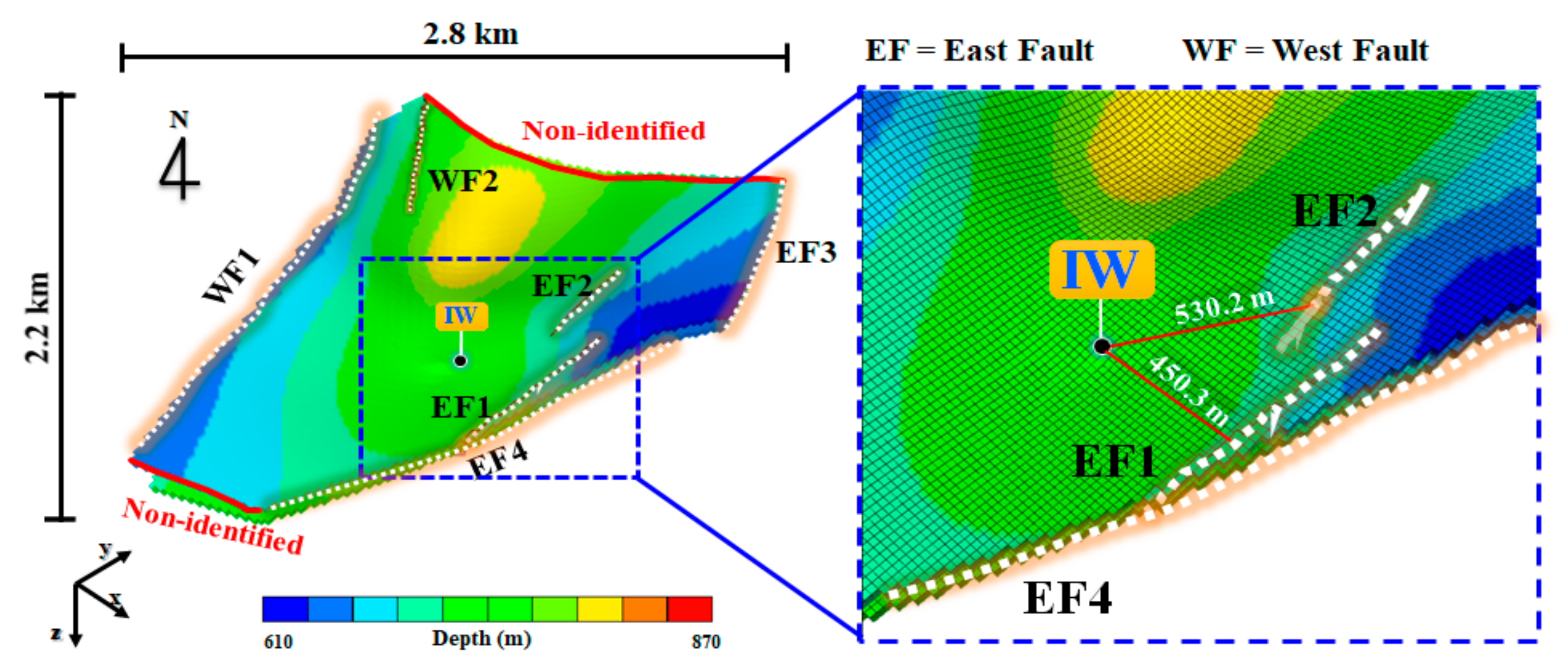
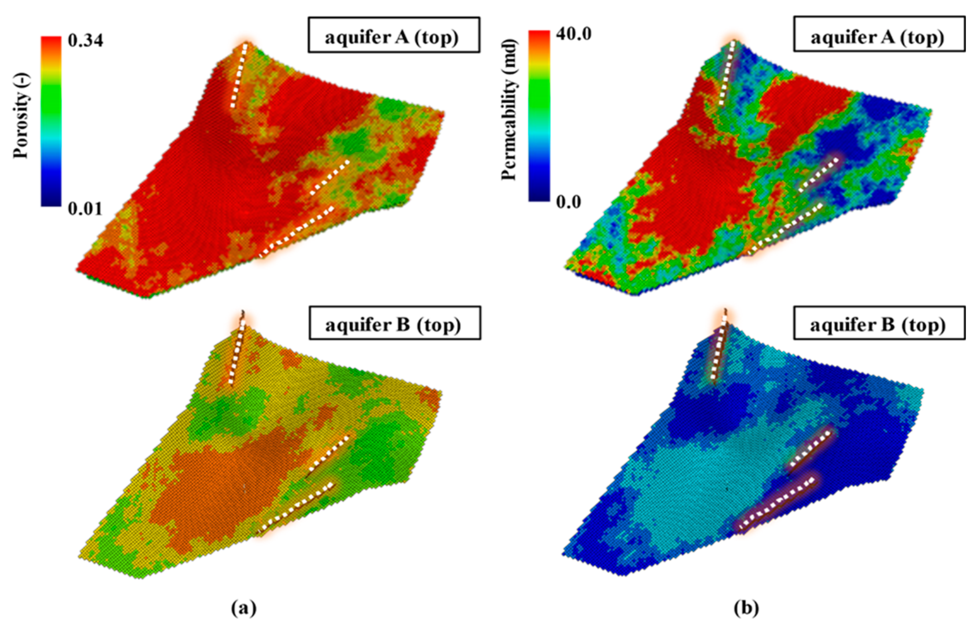
2.1. Geological Settings

The target area of this study is located at the Pohang Basin on the southeastern coast of South Korea (Figure 1). A CO₂ injection well was drilled, and about 100 tons of CO₂ were injected in 2017 as a field scale pilot test [40]. The average water depth of the target area is 15.0 m, and the depth at the injection well is 15.9 m [41]. Based on geological studies, it was found that the target formation contains coarse-grained conglomerate and sandstone at depths deeper than 740.0 m from the sea level. In addition, potential leakage of the injected CO₂ in the upper direction can be prevented with an overlying caprock of 700.0 m or thicker [42] (Figure 2a). It was found that the target formation contains two aquifer layers that were technically available for CO₂ injection and storage, aquifer A and B (Figure 2b). Aquifer A, which consists of alternating sandstone layers, has a thickness of 11.0 m, and an average permeability of 30 md. On the other hand, aquifer B contains commingled layers of sandstone, mudstone, and conglomerate. The thickness of aquifer B is 14.0 m with an average permeability of 11 md.

2.2. Three-Dimensional Geological Model Construction

A 3D geological model of the target aquifer was constructed based on seismic survey and exploration well data obtained by the Korea Institute of Geoscience and Mineral Resources (KIGAM) in 2005 [43,44] (Figure 3). The modeled area is 2.8 km by 2.2 km in the east–west and the south–north direction, respectively. As shown in Figure 3, the target aquifers become shallower as the distance from the injection well increases to the eastern and western boundaries. The number of grids is, respectively, 95 × 152 × 56 in the x-, y-, and z-(vertical) directions, including the overlying caprock and the intervening intra seal layer. The target aquifers have 24 grid-layers with a vertical length of 1 m. To improve the simulation computing speed, 32 grid-layers for the intra seal were treated as null-blocks with a permeability of 0.001 md.

According to the fault information interpreted from the seismic data, there are 6 normal faults in the target aquifers [45]. The faults are located west and east from the injection well, and were named WF1 and WF2, and EF1, EF2, EF3, and EF4, respectively. Faults WF1, EF3, and EF4 are closed boundaries that limit the crossing fluid flow. For the southern and northern boundaries of the model, no fluid flow boundary conditions were assumed for a conservative analysis in terms of CO₂ storage capacity and injectivity. The additional 3 normal faults (WF2, EF1, and EF2) are located closer to the injection well, intersecting aquifers A and B, the caprock, and the intra seal layer. In the western direction of the injection well, WF2 developed in the SE direction, and its closest point is 945.3 m away from the injection well. In the east direction, EF1 developed in the NNE-SSW direction, and its closest point is 450.3 m from the injection well. Fault EF2 is horizontally shorter than EF1, and is 530.2 m away from the injection well.

The porosity and permeability distributions used in this model are as shown in Figure 4. The porosity distribution was obtained from well logs at the injection well. The permeability distribution was obtained from the porosity distribution, determined using the Kozeny-Carman equation, which correlates the relationship between porosity and permeability. Consequently, the average porosity and permeability of the aquifer A were obtained as 32% and 30 md, respectively; aquifer B had a lower porosity and permeability of 24% and 11 md. Relative permeabilities of CO₂ and water for drainage and imbibition processes were used in the simulations with the model from [46,47], respectively.

The pore pressure and temperature conditions in the target aquifer were determined by the hydrostatic pressure (10.0 kPa/m) and local geothermal gradients (46.5 °C/km), respectively [48]. As listed in

Table 1. Properties of target layers in Pohang Basin, South Korea.

Parameter		Value	Parameter		Value
Pore pressure at 750.0 m		7.5 MPa	Temperature at 750.0 m		55.0 °C
Well bottomhole pressure (BHP)		14.0 MPa	Salinity		100,000 ppm
Fault reactivation pressure (Safety factor 80%)		14.6 MPa (11.7 MPa)	Average permeability	aquifer A	30 md
				aquifer B	11 md
Thickness	aquifer A	11.0 m	Average porosity	aquifer A	0.32
	aquifer B	14.0 m		aquifer B	0.24

, the pore pressure and temperature at the top of the model were 7.5 MPa and 55.0 °C at 750.0 m, respectively. The salinity of the aquifer was assumed as 100,000 ppm based on the reported value from the target aquifer [49].

According to a previous study, the fracture pressure at the top of the target formation is 18.2 MPa, which is expected to generate a hydraulically induced fracture [40]. However, 14.0 MPa was chosen for the operating bottomhole pressure (BHP) during the injection process, which was the maximum capacity of the compressor installed at the surface treating facility [41]. The minimum operating BHP at the relief well of 7.5 MPa was adopted, based on the hydrostatic pressure at the top of the target aquifer. In order to investigate potential fault reactivation phenomenon, the maximum pore pressure at the fault was constrained at 11.7 MPa, which was calculated from the estimated fault reactivation pressure of 14.6 MPa with a safety factor of 80% [45,50]. Another constraint implemented was injected CO₂ breakthrough, i.e., both the injection and relief wells stop operating when injected CO₂ is produced at the relief well.

3. Methodology

This section introduces methods to generate datasets for training and testing an ANN model. To develop a reliable ANN model, sufficient training datasets need to be prepared. Therefore, optimization processes were performed to generate training and testing datasets using the commercial software, CMOST. For given injection periods, the location of the relief well, and the operating conditions of both the injection and relief wells were optimized to achieve the maximum cumulative mass of injected CO₂. After the injection period, pore pressure distributions and trapping mechanisms were monitored. The total period of both the injection and monitoring processes was 300 years so as to investigate the long-term storage stability and storage efficiency. Injection scenarios of 10- and 30-years were chosen to generate the training datasets. An additional optimization process was also performed with a 20-year injection period to validate the developed model.

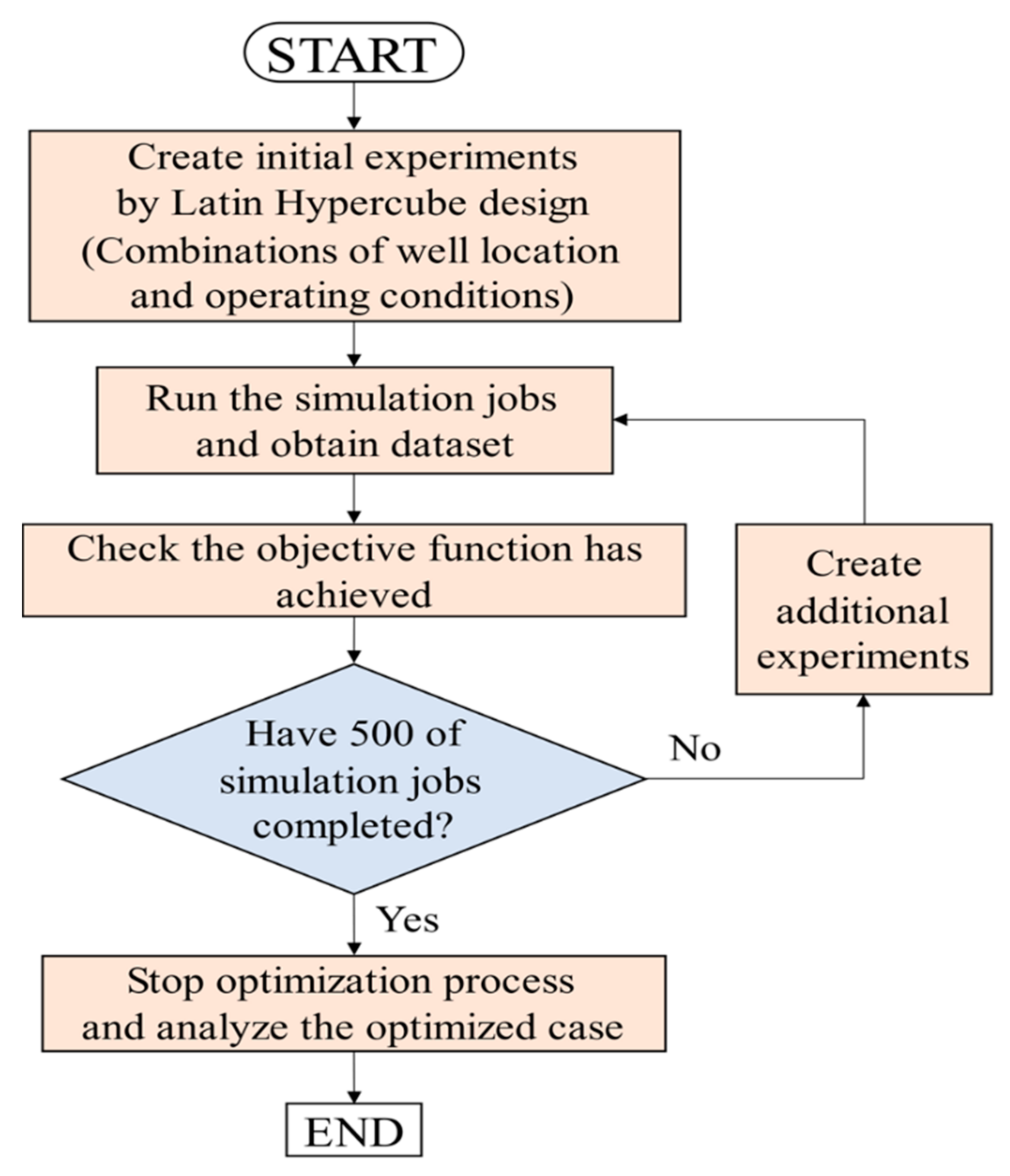
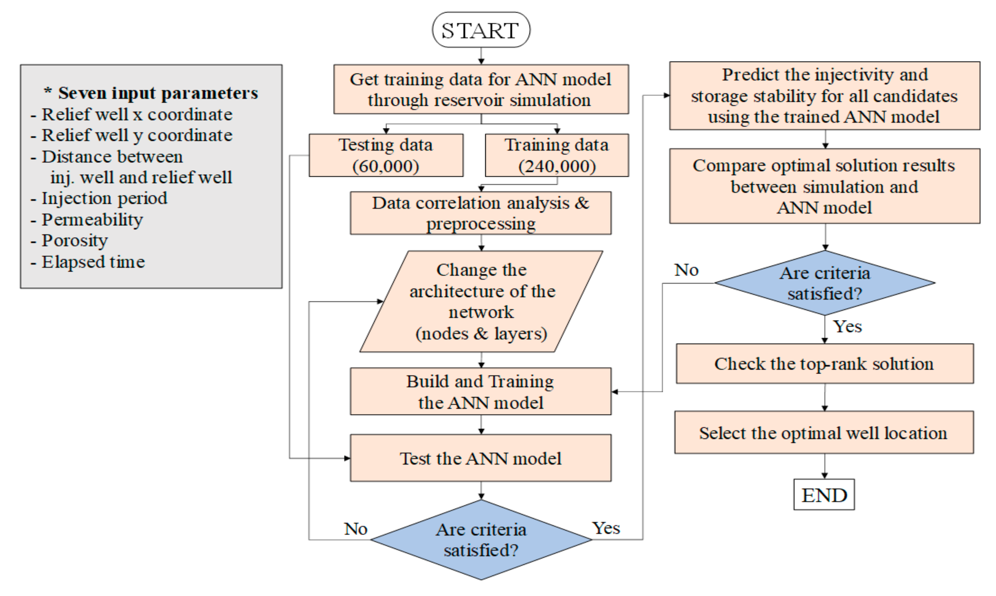
3.1. Optimization Process

The geological characteristics of the Pohang Basin are represented by multi-layered aquifers and heterogeneous reservoir properties. Moreover, the basin contains faults, which need to be taken into account for safe injection and storage design to achieve the maximum storage capacity. For example, the increased pore pressure during a CO₂ injection process may cause pre-existing fault reactivation. In addition, induced tensile fractures may occur in the vicinity of the injection well if the operating BHP exceeds the fracture pressure. Therefore, the operating conditions and the relief well location should be carefully determined, both for safe storage and storage capacity.

The relief well location and the CO₂ injection rate were chosen as the optimization parameters in an attempt to achieve maximum storage capacity. It was assumed that the relief well produces formation fluid with a constant BHP (=7.5 MPa), determined by the hydrostatic pressure, which implies that any increment in the pore pressure induced by the injection process will be removed. Once the location of the relief well was properly optimized, safe injection and storage design could be achieved with the maximum injected CO₂ mass.

The optimization process was performed with CMG CMOST and the DECE (Designed Exploration and Controlled Evolution) optimizer for three injection scenarios, a total of 300 years, i.e., 10-, 20-, and 30-year-injection period and rest was a monitoring period. In the DE stage, the optimizer generates simulation experiments through the experimental design and the Tabu search techniques, as shown in Figure 5. The experiments employ a Latin Hypercube design to generate the initial experiments, prior to the simulation run. Based on the simulation results, the optimizer determines if the objective function is achieved. During the simulation, the optimizer repeats the creation of additional experiment cases as the Tabu search technique reduces the search area. Once the targeted number of simulation jobs was reached, 500 in this study, the optimization process is completed and the optimized case was analyzed. In the CE stage, the optimizer improves the quality of the solution with a statistical analysis that tests all candidate values. While the process is being performed, the DECE algorithm checks the rejected candidate values to determine if previous decisions are still valid, and prevents the process from being trapped in a local optimal solution [51]. The steps allow the DECE to handle both continuous and discrete parameters, which is suitable for finding the optimal location of a relief well and the CO₂ injection rate in a target aquifer. In relief well optimization, the points in the two candidate sectors, A and B, contributed to the range of optimization parameters for the well location (Figure 6), with the injection rates ranging from 10 tons/day to 200 tons/day.

3.2. Storage Efficiency

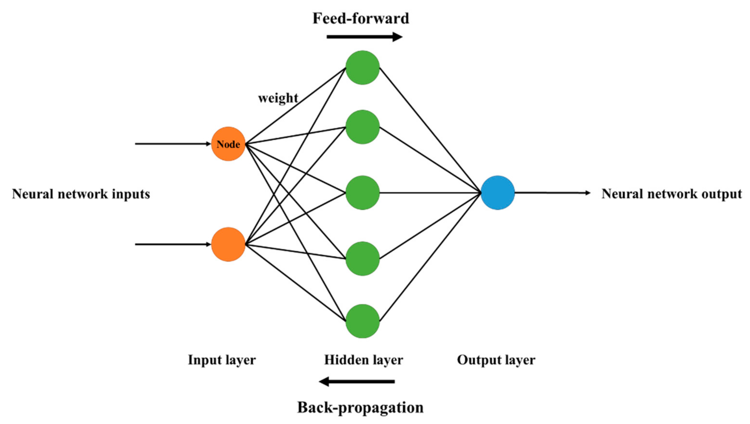
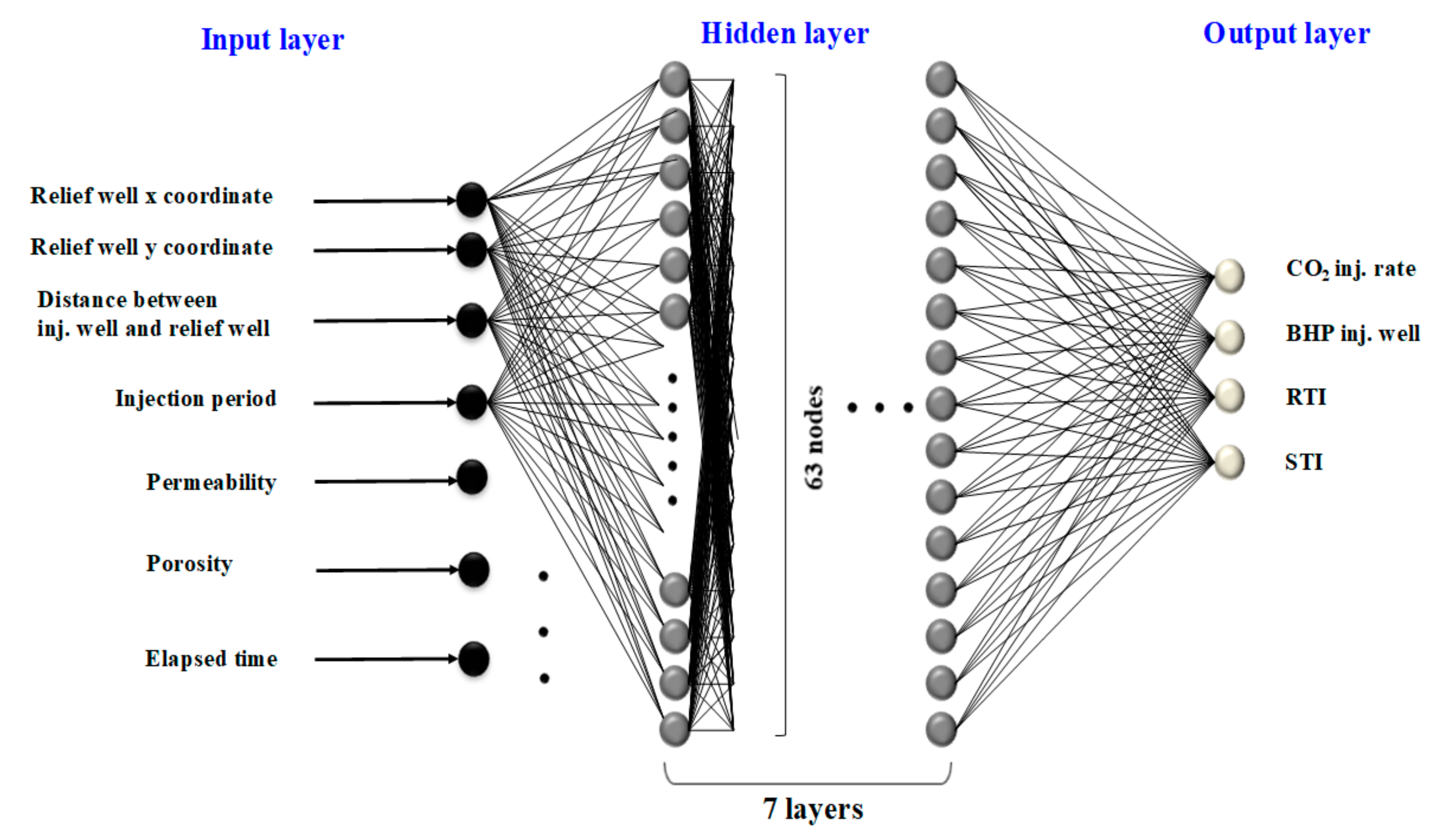
The storage efficiency in a saline aquifer depends on the CO₂ trapping mechanisms [12], i.e., the structural trapping, residual trapping, solubility trapping, and mineral trapping. Figure 7 shows the CO₂ trapping mechanisms and their contribution to the total storage efficiency. Structural trapping is characterized by the existence of a geological structure, a geometric arrangement of impermeable sealing rocks, and reservoir rocks. The contribution of structural trapping is the greatest as soon as the injection process is finished. However, it decreases over time as the other trapping mechanisms take over as the structurally trapped CO₂ is mobile and, thus, less secured. The injected CO₂ sequestrated by the residual trapping, defined by the CO₂ trapped by the capillary force, and the solubility trapping, defined by the CO₂ dissolved in the formation fluid, are considered almost permanent. The mineral trapping mechanism, which is the CO₂ conversion to carbonate minerals, such as calcite, dolomite, and siderite, is the safest in terms of stable storage of CO₂ and most permanent, its contribution is insignificant for a time period shorter than 1000 years. Therefore, in this study, residual and solubility trapping mechanisms were taken into account for the storage efficiency analysis. In order to quantify the storage efficiency, two indices—residual trapping index (RTI) and solubility trapping index (STI)—were adopted [52]. The indices were calculated as follows,

$$Residual gas trapping index \left(RTI\right) = \frac{Total mass of C{O}_2 trapped as residual gas \left(ton\right)}{Total mass of C{O}_2 injected \left(ton\right)}$$

(1)

$$Solubility gas trapping index \left(STI\right) = \frac{Total mass of C{O}_2 soluble into brine \left(ton\right)}{Total mass of C{O}_2 injected \left(ton\right)}$$

(2)

4. ANN Modeling

This section chronologically describes how to develop the ANN model for relief well optimization. In general, an ANN models consist of input, hidden, and output layers, based on a perceptron algorithm, which resembles human neurons [53]. Each layer consists of nodes, which are basic units of computation in a neural network. Each node is connected to each other using feed forward methodology that considers links for node computation. Figure 8 shows an example of a feed forward back propagation neural network with one input layer, one hidden layer, and one output layer. Each node in all layers is fully connected with weights. When the datasets of inputs and outputs are provided to the ANN with a supervised learning algorithm, it learns in a way that repeats the output from the inputs by tuning the weights: this process is referred to as training [38]. In order to train the neural network model, multi-layer feed forward back propagation methodology was adopted with a non-linear relationship between inputs and outputs. The ANN model for relief well optimization was developed using Keras with Tensor Flow [54], which is an open source machine learning framework provided by Google [55]. We created a learning neural network and developed deep learning in a sequential model as the ANN model is defined in Python with Keras as a sequence of layers.

For a better performance, it is very important to design the appropriate structure of the model, i.e., input layer, optimal number of hidden layers, optimal number of nodes in each hidden layer, appropriate activation functions, and the output layer. The ANN modeling process used in this study is schematically described in Figure 9. The seven parameters that have a significant effect on the optimal relief well design were determined for the input parameter of the model. Using the determined parameters, 1000 datasets were generated from the 10- and 30-year injection scenarios (500 datasets for each). A total of 300,000 samples with elapsed times of 300 years were extracted from the 1000 generated datasets. The generated samples were categorized into two groups, i.e., the 240,000 training and 60,000 testing datasets, which reflect 80% and 20% of the total samples, respectively. The training datasets were used to train the model by adjusting network weights and biases, and the testing datasets were used to test and to evaluate the final performance of the model. Data correlation analysis and a preprocessing process were performed to convert the optimized data into a training dataset and then an ANN model was developed while changing the hyperparameters (i.e., number of nodes and layers) of the ANN model. After the performance of the ANN model was tested, the injectivity, storage stability and storage efficiency were predicted at all points of the candidate sector of the relief well location. The predicted values at all points were verified by comparing with the simulation results. If the prediction was accurate, the calculated mass of cumulative CO₂ injection at all points of the candidate sector was analyzed and the relief well location with the maximum value was selected. The selected location was determined as the optimum position for the relief well within the candidate sector in Pohang Basin.

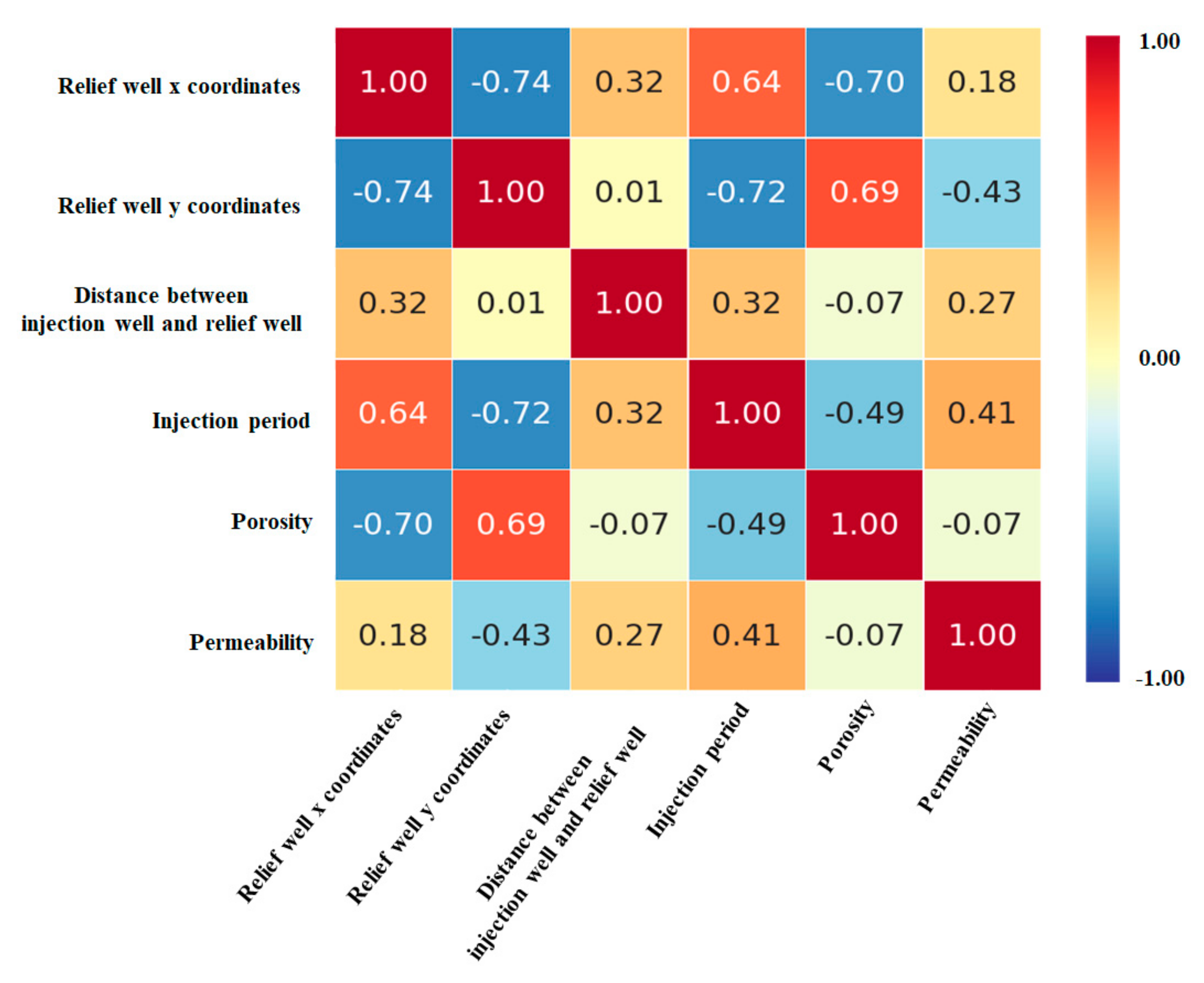
4.1. Data Correlation Analysis and Data Preprocessing

In the data correlation analysis, the dependency between the input parameters was identified to enhance the ANN model performance. If parameters that were highly dependent on each other are incorporated into input layers, the model performance would not be effective. Thus, in this study, the Pearson correlation method was adopted for data correlation analysis to identify the dependency between parameters. The Pearson’s correlation coefficient, $r_{xy}$, can be determined by,

$$r_{xy}=\frac{\sqrt{x_i{y}_i}-n\overline{x}\overline{y}}{\sqrt{\left(\sum x_i^2-n{\overline{x}}^2\right)}\sqrt{\left(\sum y_i^2-n{\overline{y}}^2\right)}}$$

(3)

where, $n$ is the sample size, $x_i$ and $y_i$ are the individual sample points indexed with $\overline{x}$ and $\overline{y}$ are the mean values of target parameters $x$ and $y$, respectively. The range of Pearson correlation coefficient $r_{xy}$ lies between −1 and 1. The coefficient value −1, 0, and 1 indicate perfectly negative correlation, no correlation, and perfectly positive correlation, respectively.

The input parameters with negligible effects on the output parameters need to be excluded from the analysis for enhancing the performance of the ANN model. Since the primary purpose of this study is to determine optimal relief well design, variables specifying the storage capacity, storage stability, and storage efficiency were chosen as the output parameters, i.e., the CO₂ injection rate, the injection well bottomhole pressure, the RTI, and STI. The most influential input parameters on the output parameters are chosen according to previous studies, which are the relief well x and y coordinates, distance between the injection and relief wells, the injection period, the reservoir average porosity, and the reservoir average permeability [25,56,57,58]. The range of selected input parameters is in

Table 2. Input parameters and their ranges in Pohang Basin, Korea.

Parameter	Minimum		Maximum
Relief well x coordinate	Sector A	33	Sector A	77
	Sector B	12	Sector B	91
Relief well y coordinate	Sector A	42	Sector A	126
	Sector B	92	Sector B	119
Distance between the injection and relief wells	100.4 m		1266.31 m
Injection period	10 years		30 years
Reservoir average porosity	0.23		0.29
Reservoir average permeability	3.63 md		18.75 md

.

The calculated Pearson correlation coefficients between the input parameters are described as a heatmap in Figure 10. The correlation magnitudes between the parameters appear to be distributed within the range from −0.74 to 0.69. It shows that the highest correlation level ($r_{xy}$ = −0.74) was found between the x and y coordinates of the relief well, while the distance between the wells and the relief well y coordinates have the smallest dependency ($r_{xy}$ = 0.01). Although no perfect correlation was found, there are 3 pairs of parameters that show relatively high dependency with the absolute Pearson’s correlation coefficient higher than 0.7: the porosity and the relief well x coordinates ($r_{xy}$ = −0.70), the injection period, and the relief well y coordinates ($r_{xy}$ = −0.72). Meanwhile, little dependencies were found over 2 pairs of parameters, the distance between the wells and the porosity ($r_{xy}$ = −0.07), and the permeability and the porosity ($r_{xy}$ = −0.07).

The 300,000 samples extracted from the optimization results should be normalized to avoid numerical overflows induced by various weights due to the differences in the units and ranges. For all the input data, the StandardScaler in the scikit-learn package was used to normalize the mean of each parameter to zero and the variance to one. In general, an ANN operates with an input layer, an optimal number of hidden layers, an optimal number of nodes in each hidden layer, a suitable activation function, and an output layer.

The rectified linear unit (ReLU) function, the most widely used activation function, was incorporated into the ANN to allow the network to learn the complex patterns of the datasets [59,60]. The ReLU function zeroes negative parameters and returns the original value for positive parameters. Adopting the function accelerates the network training speed as it decrease likelihood of gradient loss [61]. The other advantage of ReLU is sparsity, which arises when input values are negative or zero. A larger number of nodes in a layer results in a sparser representation [59]. The Adam optimizer was used for the ReLU function as an efficient stochastic gradient descent algorithm, which is a general version of gradient descent because it automatically tunes itself and provides reliable results for a wide range of problems [62].

4.2. Optimal Number of Nodes and Hidden Layers

In an ANN, a node (neuron or perceptron) is a computational unit with weighted input connections and a transfer function combining the inputs and an output connection. To create a network, nodes are organized into hidden layers between the input and output layers. Nodes on a hidden layer are directly connected to the input parameters and contribute to the output parameters. If multiple hidden layers are adopted, the number of layers and nodes are crucial for ANN model performance. Since it is not possible to analytically select the optimal number of layers and nodes, the trial and error approach was used to find the optimized multiple layer perceptron: this method is referred as to the manual search [63].

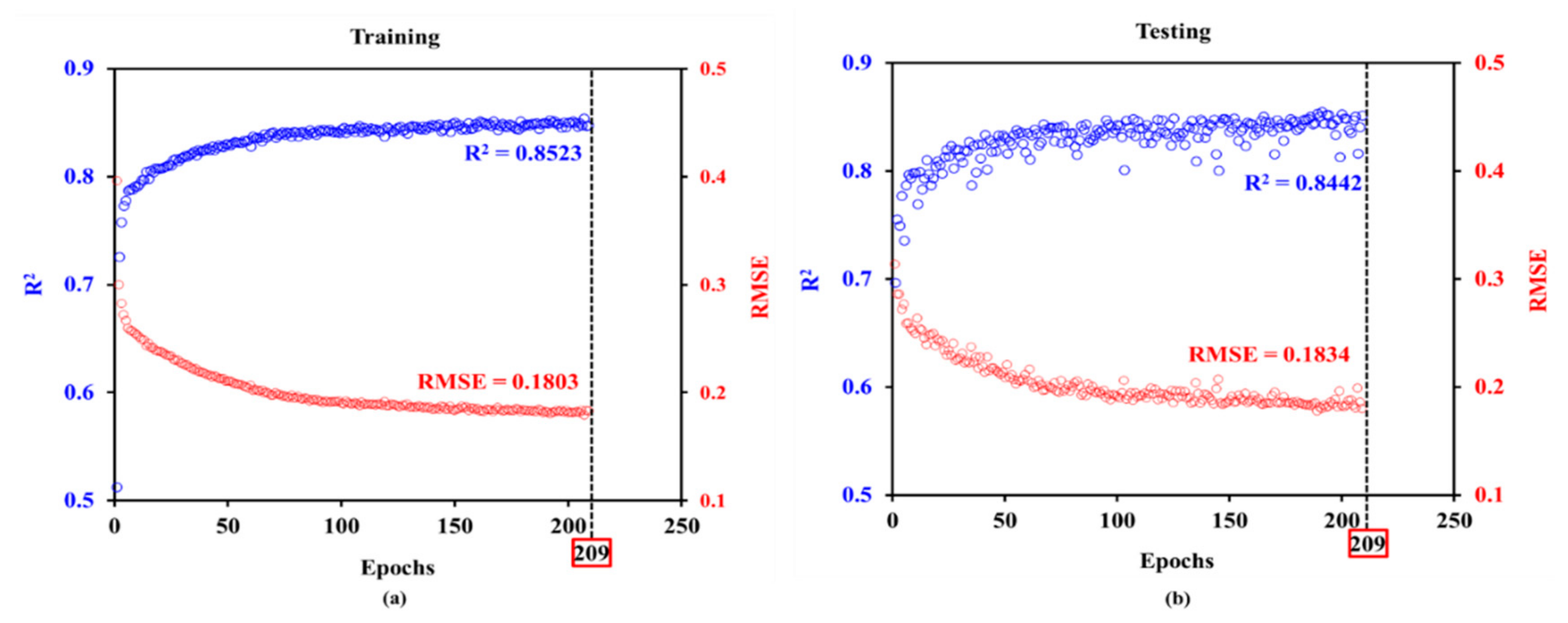
4.3. Training and Testing Procedure

The constructed ANN model was run until the desired performance was achieved. Two error functions, coefficient of determination (R²) and root mean squared error (RMSE), were adopted to evaluate the model, which are frequently used in regression analyses [64]. R² can be calculated using Equation (4).

$$R^2=1-\frac{{{\displaystyle \sum }}_{i=1}^n{\left(y_{Act,i}-{\widehat{y}}_{Pred,i}\right)}^2}{{{\displaystyle \sum }}_{i=1}^n{\left(y_{Act,i}-{\overline{y}}_{Pred,i}\right)}^2}$$

(4)

where, $y_{Act,i}$ is the actual value, ${\widehat{y}}_{Pred,i}$ is the predicted value, and ${\overline{y}}_{Pred,i}$ is the average of the predicted values. R² has a value between 0 and 1, with a value close to 1 indicating that the predicted value trend is well-fitted with the actual value.

RMSE is the standard deviation of the predicted errors and is calculated as the square root of the average squared differences between the training data and the testing data, as follows,

$$RMSE={\left[\frac{1}{n}{\displaystyle \sum }_{i=1}^n{\left(y_{Act,i}-y_{Pred,i}\right)}^2\right]}^{0.5}$$

(5)

where, $y_{Act,i}$ is the actual variable.

The RMSE determines how much the predicted values are fitted with the obtained regression model. For example, a lower RMSE value indicates that the predicted value is well-fitted with the model.

Every neural network was trained for 1000 epochs. A total if 80% of the total dataset was used for training, and 20% was used to test the model using two error functions of the R² and RMSE. The early stopping method was adopted to avoid overfitting, which is defined by a decrease in the loss of the training results with a simultaneous increase in that of the testing results [65].

5. Results and ANN Model Validation

In this section, we analyze the effects of a relief well through maximum CO₂ storage capacity in Pohang Basin. We then present the results of the optimization processes to generate the training and testing datasets, and discuss the performance and verification of the developed ANN model that optimizes the relief well.

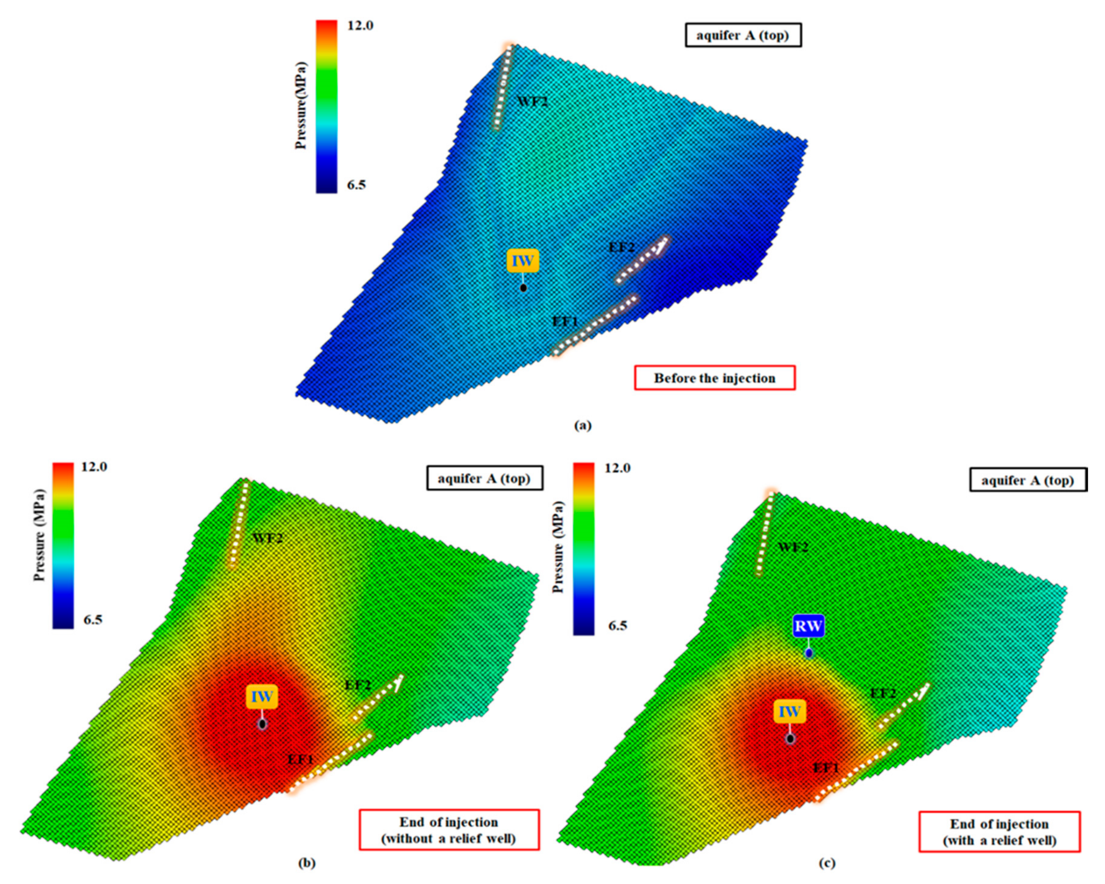
5.1. Effects of a Relief Well

In order to investigated to analyze the effectiveness of a relief well, the total CO₂ storage capacity and pore pressure distribution without a relief well were compared with the results of an installed relief well. Since a CO₂ injection well in the field was drilled, completed, and operated since 2017, the actual location and operating maximum capacity of the injection well (14.0 MPa) were implemented for the analysis. To analyze the maximum storable amount of CO₂ in the target aquifer, we primarily took the top layers of aquifers A and B into account as the layers that had the best injectivity in the Pohang Basin [66]. It was assumed that CO₂ was injected for 10 years and that this stopped when the pore pressure at faults EF1 and EF2 reached the fault reactivation pressure of 11.7 MPa.

5.1.1. Without a Relief Well

The CO₂ injection rate was optimized to maximize the mass of cumulative CO₂ injection without a relief well. The pore pressure behaviors at the faults are shown in Figure 11a. The solid and dashed curves indicate the pore pressure at the top layers of aquifers A and B, respectively. The colors specify faults EF1 (black) and EF2 (blue). The pore pressure values were measured at the closest points on faults EF1 and EF2 from the injection well. Before injection (time = 0), the pore pressure in aquifer B was higher than that of aquifer A as aquifer B is located in a deeper formation. In addition, although the pore pressure in EF1 and EF2 of aquifers A had a difference of 0.2 MPa, the pore pressure of each fault in aquifer B did not have a big difference because the depths of the faults at the top layer of aquifer B were almost identical (746.5 m, 749.8 m). As the injection process proceeded, the pore pressures in both aquifers increased. The pore pressure increase in aquifer A was larger than that of aquifer B, and the pore pressure of aquifers A exceeded aquifer B after 0.17 years and 0.21 years of injection at EF1 and EF2, respectively. This is because the average permeability of aquifer A (30 md) is higher than that of aquifer B (11 md). The injection process stopped at 6.85 years as the pore pressure of EF1 in aquifer A reached the fault reactivation pressure of 11.7 MPa, while the pore pressures at the other monitoring points were still lower. As shown in Figure 11b, which depicts the pressure distribution in aquifers A and B at the end of the injection, the pore pressure of aquifer A was distributed over a wider area than that of aquifer B due to the higher injectivity of aquifer A. Consequently, if the pore pressure in aquifer A is well managed by a relief well, it is possible to achieve a larger CO₂ storage volume with a safe injection process in terms of the potential fault reactivation.

5.1.2. With a Relief Well

In case of with a relief well, it was assumed that there was a relief well removing the pore pressure to maximize both the injectivity and capacity. As shown in the previous section, the pore pressure build-up in aquifer A was primarily focused on managing it so as to not reach the fault reactivation pressure. The location of the relief well was optimized to achieve the maximum mass of cumulative CO₂ injection. The relief well was operated with a BHP of the hydrostatic pressure, 7.5 MPa, to remove any increase in the pore pressure by the injection process. As a result, the optimal location of the relief well was 596.6 m north–east from the injection well (321.6 m and 502.5 m in the x- and y-direction, respectively) (Figure 12). In addition, it was found that the depth of the perforated interval of the relief well was optimized to be deeper (52.8 m) than that of the injection well to prevent CO₂ breakthrough. Figure 13a shows the pore pressure at the top layers of each aquifer at faults EF1 and EF2 during the injection process with a relief well. Although the initial pore pressures (t = 0) at aquifer A were lower than those of aquifer B, the pore pressures in aquifer A exceeded at time 0.17 years and 0.5 years in aquifer B at faults EF1 and EF2, respectively. However, it shows that the pore pressure of fault EF1 in A reached the fault reactivation pressure in 7.84 years. In other words, operation of the relief well extended the injection process for 1 year (365 days). When the process is finished, the pore pressure at EF1 of aquifer A was decreased and stabilized at 11.2 MPa. As shown in Figure 13b, which visualizes the pressure distribution at the end of injection in the top layers of aquifers A and B, the pore pressure at aquifer A was effectively managed by the relief well. Therefore, it was concluded that the installment and operation of the relief well effectively manage the pore pressure in aquifer A and that more CO₂ can be injected for a longer period of time.

5.1.3. Comparison without and with a Relief Well

Based on the simulation studies focusing on the existence of the relief well, it was found that the pressure build-up can be effectively managed by a relief well and that a safe injection process can be achieved, although there are potentially reactivatable faults. With the same operating BHP of 14.0 MPa, the injection rates, total storage capacity, and pore pressure distribution were taken into account to analyze the efficiency of the relief well.

The injection rates of both cases are illustrated in Figure 14. The injection rates without and with the relief well are, respectively, shown with solid and dashed curves. As soon as the injection process initiates, the injection rates in both cases increased sharply. When there is a relief well installed and operated, the maximum rate of 80 tons/day was achieved in 0.92 years, while it took 1.1 years without a relief well to reach the maximum rate. In addition, this shows that the rate with a relief well after the peak maintains longer than that of the ‘without a relief well’ case. This is because the relief well provides more injection capability. Therefore, the average injection rate with the relief well was 75 tons/day, which is 3 tons/day higher than that of the no-relief well case. Thus, the total CO₂ storage capacity with a relief well (215 kton) was 19.44% higher compared to the “without a relief well” case. Consequently, operating a relief well can provide more injection capability, which may lead to the larger total mass of injected CO₂.

Effects of the relief well can be found from the pore pressure distribution after the injection process in Figure 15. Note that the distribution of top of aquifer A is only shown for comparison. Before the injection, the pore pressure, determined by the hydrostatic pressure gradient, is in the range between 6.5 and 8.5 MPa (Figure 15a). When the injection process without a relief well is finished at 6.85 years, the pore pressure of aquifer A was increased, with the maximum concentrated location found at the injection well (Figure 15b). Moreover, a high pore pressure concentration was observed at fault EF1, which was expected to be reactivated and caused the termination of the injection. However, as shown in Figure 15c, it was found that the pore pressure build-up in aquifer A was effectively managed with the relief well as the injection period was extended to 7.84 years. Therefore, it was concluded that installing of a relief well to relieve the pore pressure may be an effective solution to manage pore pressure for a safe injection design and to maximize the cumulative mass of injected CO₂.

5.2. Optimization for Vairous Scenarios

In order to generate sufficient training and testing datasets, optimization processes were performed. For given injection periods, the location of the relief well and the operating conditions of both the injection and relief wells were optimized to achieve the maximum cumulative mass of injected CO₂. After the injection period, the pore pressure distributions and trapping mechanisms were monitored. A total of 300 years of injection and monitoring periods were selected to investigate the long-term storage stability and storage efficiency. The injection scenarios of 10 years and 30 years were chosen to generate the training datasets. Additional optimization process was also performed with a 20-year injection period to validate the developed ANN model.

Figure 16 shows the optimized location of the relief well for each injection period. When the CO₂ was injected for 10 years, the optimum location of the relief well was located 596.6 m north–east from the injection well (321.6 m and 502.5 m in the x- and y-direction, respectively) for the maximum mass of cumulative CO₂ injection. The reason for this was that the injection period was relatively short, and the injection rate was highly optimized and then pressure build-up occurred rapidly during the injection period. Thus, in order to manage the pore pressure due to CO₂ injection, the location of the relief well was optimized near the injection well. In addition, it was found that the relief well was located deeper (52.8 m) than the position of the injection well to prevent CO₂ breakthrough. For the cases of 20- and 30-year injection, the location of the relief well was located at 800.5 m and 767.5 m away from the injection well, 623.1 m and 502.5 m in the x- direction and 502.5 m and 542.7 m in the y- direction, respectively. The reason for this was that the location of the relief well was optimized for areas with high permeability to facilitate water production. In general, a higher permeability resulted in a higher water production efficiency, which means that pressure control through the water production is easier [67].

The injection rates during the injection periods are shown in Figure 17a. The solid, dashed and dotted curves indicate the rates for 10-, 20- and 30-year injection periods, respectively. The optimized injection rate for the 10-year injection scenario is 60 tons/day, while an injection rate of 40 tons/day is expected to be optimum for the 20- and 30-year injection periods. It was found that the CO₂ was injected as planned for the 10- and 20-year injection scenarios. When the 30-year injection scenario was adopted, the injection was unexpectedly terminated at 22 years (red arrow in Figure 17a). In order to identify what caused the unexpected termination, occurrence of the fault reactivation and the CO₂ breakthrough phenomenon were closely investigated. Figure 17b indicates the pore pressure at fault EF1 (black curves) and the CO₂ production rate at the relief well (blue curve). Since the pore pressure build-up is most severe at the top layer of aquifer A, that particular location was taken into account for the analysis. According to the pore pressure behaviors, it appears that the pressure did not reach the fault reactivation pressure for all the injection scenarios. However, it was found that the injected CO₂ started to be produced at the relief well at 22 years when the 30-year injection scenario was chosen (blue dotted curve in Figure 17b). The cumulative mass of injected CO₂ for the 10-, 20-, and 30-year injection periods ere 218, 292, and 332 kton. As the injection period extended, the cumulative injection mass increased. In addition, the increment of the cumulative mass was 33.94% (74 kton), when the injection period was increased from 10 years to 20 years, while it was increased only 13.7% (40 kton) if the period was extended from 20 years to 30 years. This is because the injection process was unexpectedly terminated at 22 years by the CO₂ breakthrough phenomenon and was not performed for the designed period of time. Therefore, it was concluded that a safe injection process is crucial for total storage capacity.

Moreover, the storage efficiency for the monitoring phase was investigated with the trapping mechanisms. As shown in Figure 18, the residual and solubility trapping indices (RTI and STI) were decreased during the injection period because the injected CO₂ diffuses via the pressure gradient. However, after the end of the injection, not only was the injected CO₂ trapped through pore spaces by gravitational, viscous, and capillary effects, but it also dissolved in brine, which eventually increased the residual and solubility trapping indices [49,68].

5.3. Architecture and Validation of the ANN Model

5.3.1. ANN Model Performance

To determine the optimal number of layers and nodes, nodes and hidden layers were respectively incremented seven and one at a round until we obtained the best performance with the network structure. As shown in Figure 19a, overfitting was detected at 63 nodes when the loss (RMSE) is the smallest and then rises afterwards. In the same manner, the optimal number of hidden layers was determined as seven, where it showed the best learning performance (Figure 19b). Consequently, it was concluded that the final optimized architecture of the ANN model contained 63 nodes with seven hidden layers, as shown in Figure 20.

Figure 21 shows the R² and RMSE trends during the training and testing of the constructed ANN model. Blue and red dots represent the R² and RMSE at each epoch, respectively. As shown in Figure 21, using the R² in the training and testing of the model, we obtained performances of 0.8523 and 0.8442, respectively, at epoch 209 when the model was stopped early. In addition, the RMSE in the training and testing of the model converged on 0.1803 and 0.1834, respectively, at the 209th iteration.

5.3.2. ANN Model Validation

In this section, the optimization data for the 20-year injection scenario was used to validate the ANN model using two error functions, R² and RMSE. Figure 22 shows the CO₂ injection rate for 300 years, determined by the predicted model (ANN; red) and the validation model (simulation; blue). Although the two models initially yield a gap and at 20 years, it was found that the rate was well-predicted as it showed an R² and RMSE of 0.9982 and 0.6681, respectively. In addition, R² and RMSE values calculated from the injection well BHP show great acceptance with 0.9828 and 0.0497, respectively. Especially for the monitoring phase, the ANN accurately predicted BHP during the monitoring phase. When the analysis was extended to the trap mechanisms, an R² of 0.9927 and an RMSE of 0.0136 for RTI, as well as an R² of 0.9607 and RMSE of 0.0085 for STI were achieved, which implies that the developed ANN model has great accuracy in the prediction of trap mechanisms. On the other hand, the difference in the total CO₂ storage capacity was only 0.68% (2 kton), as the ANN and the simulation predicted 294 kton and 292 kton of CO₂ could be injected for 20 years, respectively. The predicted location of the relief well only had a distance of 20.1 m based on the ANN and simulation models (Figure 23).

6. Discussion

Geological storage of CO₂ is one of the most promising methods for greenhouse gas reduction. Due to the Paris Agreement, which specifies national goals for the reduction of CO₂ emissions, to maximize injectivity and capacity should be the primary objectives for CCS design. Therefore, operating a relief well is an effective method to relieve reservoir pressure to enhance the injection capacity and allow safe injection design. Although this study primarily focuses on the maximum CO₂ storage capacity, the cost of drilling and operating a relief well can be incorporated into a detailed analysis. Unless there is an available well to be repurposed as the relief well, i.e., when a depleted hydrocarbon reservoir with multiple wells is available, the cost of drilling needs to be taken into account. If implemented with a certified emission reduction, economic analysis can provide for more reliable analyses. In the future, economic analysis with the cost of the relief well installation and operation will be incorporated into further investigations. In addition, this goes beyond the on-site pilot test conducted in this study and conducts an economic analysis that is applicable in an actual commercial field. Through this research, we will evaluate the most economically profitable operating mechanism in an actual commercial field, and proceed with research to find the optimal relief well design through economic analysis.

Based on the results, the location of the relief well is a very crucial parameter for both CO₂ storage capacity and the safe injection process. It was found that the relief well was located in a high permeability area, which implies that the effect of the relief well should be transmitted fast enough to effectively relieve the pore pressure. The results present that a CO₂ breakthrough phenomenon may occur when the relief well is operating during the injection process and appropriate design needs to be performed accordingly in advance.

A more sophisticated adjustment of the injection scheme may enhance the injectivity and capacity. Instead of adopting constant injection and production rates, fine adjustment of the rates and schedule can be implemented. For example, seasonal rate changes can be an option. Especially in winter, if the target aquifer is located offshore, the possibility of subsea hydrate formation in the tubing needs to be investigated with the seasonal change in the tidal currents. Switching an injection well with a relief well may provide flexibility to the operational strategy, which would also be very helpful to overcome unpredictable hazards.

Since the ANN model of the present study was developed using the optimization results from the actual field, the training datasets and the model represent unique values from the field. Thus, it is not suitable to compare the model outcome with other published data. Meanwhile, optimal relief well design is reliably applicable for the studied area, Pohang Basin.

The performance of an ANN model has a major role in the speed, accuracy and applicability for analyses of geological CO₂ storage. Recently, more advanced hyperparameters optimization methods to enhance the performance of ANN models have been developed, such as genetic algorithms (GA), particle swarm optimization (PSO), and Bayesian optimization. Although the current status is very preliminary, more compact and time-efficient investigations will be available in the near future. Future work of this study aims at this target, to achieve better reliability and precision over less time and computing power.

7. Conclusions

An artificial neural network (ANN) model has been developed for an optimal relief well design, using information such as the location and operating conditions, which maximize CO₂ storage capacity in Pohang Basin, South Korea. Based on the observations, the following conclusions have been drawn:

• Based on the comparisons made for with or without relief well cases, the average injection rate was 3 tons/day higher if a relief well is operated. In addition, it was found that the relief well extended the injection period by 0.99 years and increased the CO₂ storage capacity by 19.44% (215 kton).
• To generate training datasets for the input and output nodes in the ANN model, the operating conditions of both wells and the location of the relief well were optimized to achieve the maximum cumulative mass of the injected CO₂. It was found that the cumulative mass for the 10-, 20-, and 30-year injection periods were 218, 292, and 332 kton, respectively. Therefore, the cumulative injection mass increased by 33.94% (74 kton) and 13.7% (40 kton) as the injection period was extended from 10 to 20 years and from 20 to 30 years, respectively. Consequently, it was concluded that 20 years of injection with the relief well would be the best scenario in terms of safe and effective storage in Pohang Basin.
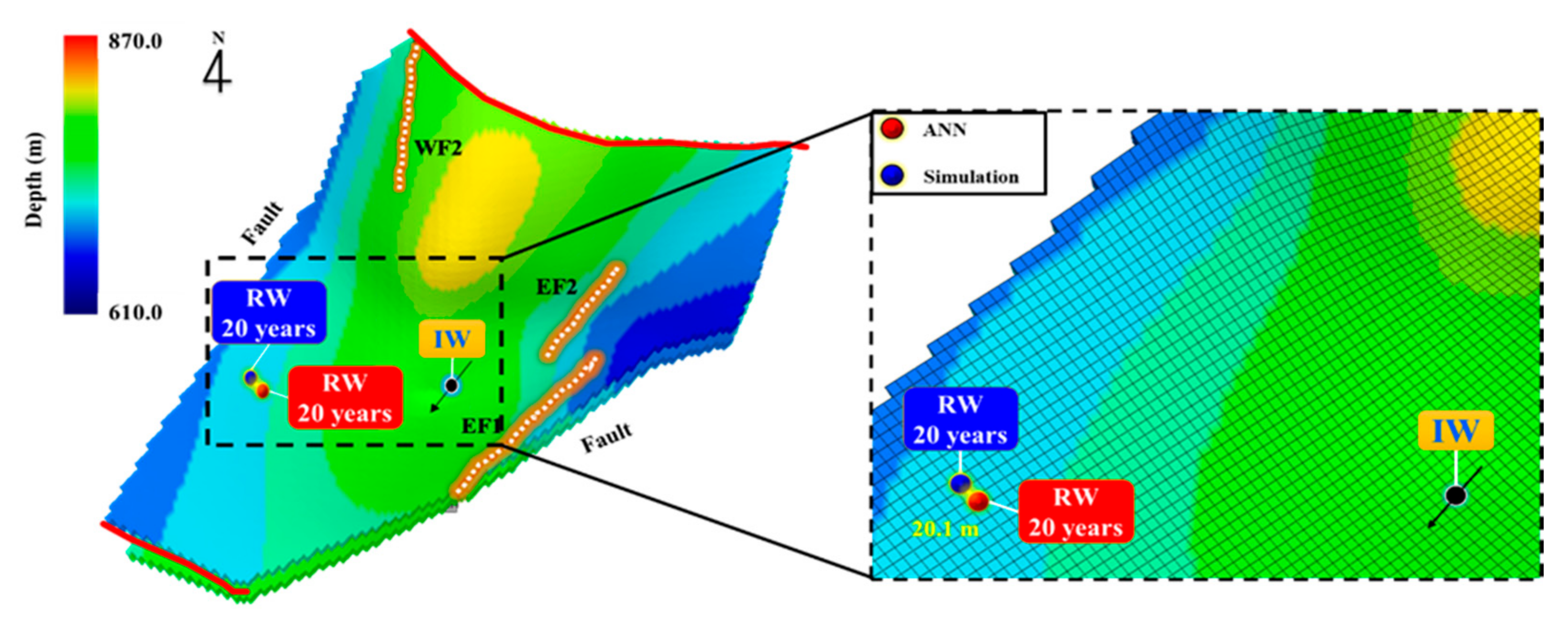
• The ANN model was developed with datasets of 10- and 30-year injection scenarios and validated with that of the 20-year scenario. The optimal architecture of the model consisted of 63 nodes and seven hidden layers at 209 iterations. When the predicted data were compared to the validation data, the ANN model reliably predicted the result with an R² of 0.9982 and RMSE of 0.6681 for the CO₂ injection rate, and an R² of 0.9828 and RMSE of 0.0497 for the injection well BHP. In addition, the developed ANN model had great accuracy in the prediction of the trapping indices, with an R² of 0.9927 and RMSE of 0.0136 for the RTI, and an R² of 0.9607 and RMSE of 0.0085 for the STI, respectively. The total CO₂ storage capacity and the relief well location were also accurately predicted with only a 0.68% difference (2 kton) and a distance of 20.1 m, respectively.

Consequently, it was concluded that the developed ANN model can accurately optimize relief well design and evaluate storage efficiency in Pohang Basin, South Korea. In addition, the ANN model can be a robust tool to optimize relief well design and to evaluate storage efficiency for successful CO₂ sequestration without a time-consuming reservoir simulation at the early stages of a CCS project.

References

1. In, I.; Metz, B.; Davidson, O.; de Coninck, H.; Loos, M.; Meyer, L. IPCC Special Report on Carbon Dioxide Capture and Storage: Prepared by Working Group III of the Intergovernmental Panel on Climate Change; Metz, B., Davidson, O., de Conink, H., Loos, M., Meyer, L., Eds.; Intergovernmental Panel on Climate Change: Geneva, Switzerland, 2005. [Google Scholar]
2. Whittaker, S.; Rostron, B.; Hawkes, C.; Gardner, C.; White, D.; Johnson, J.; Chalaturnyk, R.; Seeburger, D. A decade of CO2 injection into depleting oil fields: Monitoring and research activities of the IEA GHG Weyburn-Midale CO2 Monitoring and Storage Project. Energy Procedia 2011, 4, 6069–6076. [Google Scholar] [CrossRef] [Green Version]
3. Wollenweber, J.; Alles, S.a.; Kronimus, A.; Busch, A.; Stanjek, H.; Krooss, B.M. Caprock and overburden processes in geological CO2 storage: An experimental study on sealing efficiency and mineral alterations. Energy Procedia 2009, 1, 3469–3476. [Google Scholar] [CrossRef] [Green Version]
4. Singh, V.P.; Cavanagh, A.; Hansen, H.; Nazarian, B.; Iding, M.; Ringrose, P.S. Reservoir modeling of CO2 plume behavior calibrated against monitoring data from Sleipner, Norway. In Proceedings of the SPE Annual Technical Conference and Exhibition, Florence, Italy, 19–22 September 2010. [Google Scholar]
5. Rutqvist, J.; Birkholzer, J.; Cappa, F.; Tsang, C.F. Estimating maximum sustainable injection pressure during geological sequestration of CO2 using coupled fluid flow and geomechanical fault-slip analysis. Energy Convers. Manag. 2007, 48, 1798–1807. [Google Scholar] [CrossRef] [Green Version]
6. Arts, R.; Chadwick, A.; Eiken, O.; Thibeau, S.; Nooner, S. Ten years’ experience of monitoring CO2 injection in the Utsira Sand at Sleipner, offshore Norway. First Break 2008, 26. [Google Scholar] [CrossRef]
7. Ruiz, H.; Agersborg, R.; Hille, L.T.; Lien, M.; Lindgård, J.; Vatshelle, M. Monitoring Offshore CO2 Storage Using Time-lapse Gravity and Seafloor Deformation; European Association of Geoscientists & Engineers: Houten, The Netherlands, 2017. [Google Scholar] [CrossRef]
8. Masson-Delmotte, V.; Zhai, P.; Pörtner, H.-O.; Roberts, D.; Skea, J.; Shukla, P.R.; Pirani, A.; Moufouma-Okia, W.; Péan, C.; Pidcock, R. Global warming of 1.5 C. IPCC Spec. Rep. Impacts Glob. Warm. 2018, 1, 1–9. [Google Scholar]
9. Crippa, M.; Oreggioni, G.; Guizzardi, D.; Muntean, M.; Schaaf, E.; Lo Vullo, E.; Solazzo, E.; Monforti-Ferrario, F.; Olivier, J.; Vignati, E. Fossil CO2 and GHG Emissions of All World Countries; Publication Office of the European Union: Luxembourg, 2019. [Google Scholar]
10. Cho, G.; Cho, H.; Park, N. A Study on Implementation and Deriving Future Tasks of ‘The Korean National CCS Master Action Plan’. J. Clim. Chang. Res. 2016, 7, 237–247. [Google Scholar] [CrossRef]
11. Kwon, Y.K.; Shinn, Y.J. Suggestion for technology development and commercialization strategy of CO2 capture and storage in Korea. Econ. Environ. Geol. 2018, 51, 381–392. [Google Scholar] [CrossRef]
12. Metz, B. Carbon Dioxide Capture and Storage: IPCC Special Report. Summary for Policymakers, a Report of Working Group III of the IPCC; Technical Summary, a Report Accepted by Working Group III of the IPCC but Not Approved in Detail; World Meteorological Organization: Geneva, Switzerland, 2006. [Google Scholar]
13. Bachu, S. Sequestration of CO2 in geological media: Criteria and approach for site selection in response to climate change. Energy Convers. Manag. 2000, 41, 953–970. [Google Scholar] [CrossRef]
14. Bachu, S. CO2 storage in geological media: Role, means, status and barriers to deployment. Prog. Energy Combust. Sci. 2008, 34, 254–273. [Google Scholar] [CrossRef]
15. Kaldi, J.; Gibson-Poole, C. Storage Capacity Estimation, Site Selection and Characterisation for CO2 Storage Projects; CO2CRC, Report No. RPT08-1001; Cooperative Research Centre for Greenhouse Gas Technologies: Canberra, Australia, 2008. [Google Scholar]
16. Bachu, S. Comparison between Methodologies Recommended for Estimation of CO2 Storage Capacity in Geological Media; Sequestration Leadership Forum, Phase III Report; Carbon Sequestration Leadership Forum: Washington, DC, USA, 2008. [Google Scholar]
17. Morris, J.P.; Detwiler, R.L.; Friedmann, S.J.; Vorobiev, O.Y.; Hao, Y. The large-scale geomechanical and hydrogeological effects of multiple CO2 injection sites on formation stability. Int. J. Greenh. Gas Control 2011, 5, 69–74. [Google Scholar] [CrossRef]
18. Dauben, D.L.; Froning, H.R. Development and Evaluation of Micellar Solutions To Improve Water Injectivity. J. Pet. Technol. 2017, 23, 614–620. [Google Scholar] [CrossRef]
19. Sloat, B.F.; Larsen, D. How To Stabilize Clays and Improve Injectivity. In Proceedings of the SPE Rocky Mountain Regional Meeting, Casper, WY, USA, 21 May 1984; p. 12. [Google Scholar]
20. Goodarzi, S.; Settari, A.; Zoback, M.; Keith, D.W. Thermal Effects on Shear Fracturing and Injectivity During CO2 Storage. In Proceedings of the ISRM International Conference for Effective and Sustainable Hydraulic Fracturing, Brisbane, Australia, 20–22 May 2013; p. 14. [Google Scholar]
21. Li, S.; Zhang, Y.; Zhang, X. A study of conceptual model uncertainty in large-scale CO2 storage simulation. Water Resour. Res. 2011, 47. [Google Scholar] [CrossRef] [Green Version]
22. Bergmo, P.E.S.; Grimstad, A.-A.; Lindeberg, E. Simultaneous CO2 injection and water production to optimise aquifer storage capacity. Int. J. Greenh. Gas Control 2011, 5, 555–564. [Google Scholar] [CrossRef]
23. Tiamiyu, O.M.; Nygaard, R.; Bai, B. Effect of Aquifer Heterogeneity, Brine Withdrawal, and Well-Completion Strategy on CO2 Injectivity in Shallow Saline Aquifer. In Proceedings of the SPE International Conference on CO2 Capture, Storage, and Utilization, New Orleans, LA, USA, 10–12 November 2010; p. 15. [Google Scholar]
24. Buscheck, T.A.; Sun, Y.; Chen, M.; Hao, Y.; Wolery, T.J.; Bourcier, W.L.; Court, B.; Celia, M.A.; Julio Friedmann, S.; Aines, R.D. Active CO2 reservoir management for carbon storage: Analysis of operational strategies to relieve pressure buildup and improve injectivity. Int. J. Greenh. Gas Control 2012, 6, 230–245. [Google Scholar] [CrossRef]
25. Buscheck, T.A.; Bielicki, J.M.; White, J.A.; Sun, Y.; Hao, Y.; Bourcier, W.L.; Carroll, S.A.; Aines, R.D. Managing Geologic CO2 Storage with Pre-injection Brine Production in Tandem Reservoirs. Energy Procedia 2017, 114, 4757–4764. [Google Scholar] [CrossRef]
26. Cihan, A.; Birkholzer, J.T.; Bianchi, M. Optimal well placement and brine extraction for pressure management during CO2 sequestration. Int. J. Greenh. Gas Control 2015, 42, 175–187. [Google Scholar] [CrossRef] [Green Version]
27. Hwang, J.; Baek, S.; Lee, H.; Jung, W.; Sung, W. Evaluation of CO2 storage capacity and injectivity using a relief well in a saline aquifer in Pohang basin, offshore South Korea. Geosci. J. 2016, 20, 239–245. [Google Scholar] [CrossRef]
28. Kim, M.; Shin, H. Application of a dual tubing CO2 injection-water production horizontal well pattern for improving the CO2 storage capacity and reducing the CAPEX: A case study in Pohang basin, Korea. Int. J. Greenh. Gas Control 2019, 90, 102813. [Google Scholar] [CrossRef]
29. Mohaghegh, S. Virtual-Intelligence Applications in Petroleum Engineering: Part 1—Artificial Neural Networks. J. Pet. Technol. 2000, 52, 64–73. [Google Scholar] [CrossRef]
30. Guler, B.; Ertekin, T.; Grader, A.S. An Artificial Neural Network Based Relative Permeability Predictor. J. Can. Pet. Technol. 2003, 42, 9. [Google Scholar] [CrossRef]
31. Jeirani, Z.; Mohebbi, A. Estimating the initial pressure, permeability and skin factor of oil reservoirs using artificial neural networks. J. Pet. Sci. Eng. 2006, 50, 11–20. [Google Scholar] [CrossRef]
32. Azizi, S.; Awad, M.M.; Ahmadloo, E. Prediction of water holdup in vertical and inclined oil–water two-phase flow using artificial neural network. Int. J. Multiph. Flow 2016, 80, 181–187. [Google Scholar] [CrossRef]
33. Zhong, Z.; Sun, A.Y.; Jeong, H. Predicting CO2 Plume Migration in Heterogeneous Formations Using Conditional Deep Convolutional Generative Adversarial Network. Water Resour. Res. 2019, 55, 5830–5851. [Google Scholar] [CrossRef]
34. Hamam, H.; Ertekin, T. A generalized continuous carbon dioxide injection design and screening tool for naturally fractured reservoirs of varying oil compositions. In Proceedings of the SPE EOR Conference at Oil and Gas West Asia, Muscat, Oman, 26–28 March 2018. [Google Scholar]
35. Jamali, B.; Haghighat, E.; Ignjatovic, A.; Leitão, J.P.; Deletic, A. Machine learning for accelerating 2D flood models: Potential and challenges. Hydrol. Process. 2021, 35, e14064. [Google Scholar] [CrossRef]
36. Taherdangkoo, R.; Tatomir, A.; Taherdangkoo, M.; Qiu, P.; Sauter, M. Nonlinear Autoregressive Neural Networks to Predict Hydraulic Fracturing Fluid Leakage into Shallow Groundwater. Water 2020, 12, 841. [Google Scholar] [CrossRef] [Green Version]
37. Sipöcz, N.; Tobiesen, F.A.; Assadi, M. The use of Artificial Neural Network models for CO2 capture plants. Appl. Energy 2011, 88, 2368–2376. [Google Scholar] [CrossRef]
38. Song, Y.; Sung, W.; Jang, Y.; Jung, W. Application of an artificial neural network in predicting the effectiveness of trapping mechanisms on CO2 sequestration in saline aquifers. Int. J. Greenh. Gas Control 2020, 98, 103042. [Google Scholar] [CrossRef]
39. Wen, G.; Tang, M.; Benson, S.M. Towards a predictor for CO2 plume migration using deep neural networks. Int. J. Greenh. Gas Control 2021, 105, 103223. [Google Scholar] [CrossRef]
40. Kwon, Y.K.; Chang, C.; Shinn, Y. Security and Safety Assessment of the Small-scale Offshore CO2 Storage Demonstration Project in the Pohang Basin. J. Eng. Geol. 2018, 28, 217–246. [Google Scholar]
41. Won, K.-S.; Lee, D.-S.; Kim, S.-J.; Choi, S.-D. Drilling and Completion of CO2 Injection Well in the Offshore Pohang Basin, Yeongil Bay. J. Eng. Geol. 2018, 28, 193–206. [Google Scholar] [CrossRef]
42. Choi, B.-Y.; Park, Y.-C.; Shinn, Y.-J.; Kim, K.-Y.; Chae, G.-T.; Kim, J.-C. Preliminary results of numerical simulation in a smail-scale CO2 injection pilot site: 1. Prediction of CO2 plume migration. J. Geol. Soc. Korea 2015, 51, 487–496. [Google Scholar] [CrossRef]
43. Song, C.; Son, M.; Sohn, Y.; Han, R.; Shinn, Y.; Kim, J.C. A study on potential geologic facility sites for carbon dioxide storage in the Miocene Pohang Basin, SE Korea. J. Geol. Soc. Korea 2015, 51, 53–66. [Google Scholar] [CrossRef]
44. Cheong, S.; Koo, N.; Kim, Y.; Lee, H.; Kim, B.; Shinn, Y. Case Study of Seismic Surveying and Data Processing for Small-scale Carbon Capture and Storage in the Pohang Basin. In Proceedings of the Near Surface Geoscience 2016—22nd European Meeting of Environmental and Engineering Geophysics, Barcelona, Spain, 4–8 September 2016; p. cp-495-00034. [Google Scholar]
45. Lee, H.; Shinn, Y.J.; Ong, S.H.; Woo, S.W.; Park, K.G.; Lee, T.J.; Moon, S.W. Fault reactivation potential of an offshore CO2 storage site, Pohang Basin, South Korea. J. Pet. Sci. Eng. 2017, 152, 427–442. [Google Scholar] [CrossRef]
46. Sung, W.M.; Lee, Y.S.; Kim, K.H.; Jang, Y.H.; Lee, J.H.; Yoo, I.H. Investigation of CO2 behavior and study on design of optimal injection into Gorae-V aquifer. Environ. Earth Sci. 2011, 64, 1815–1821. [Google Scholar] [CrossRef]
47. Land, C.S. Calculation of imbibition relative permeability for two-and three-phase flow from rock properties. Soc. Pet. Eng. J. 1968, 8, 149–156. [Google Scholar] [CrossRef]
48. Lee, T.J.; Song, Y.; Park, D.-W.; Jeon, J.; Yoon, W.S. Three dimensional geological model of Pohang EGS pilot site, Korea. In Proceedings of the World Geothermal Congress, Melbourne, Australia, 19–25 April 2015. [Google Scholar]
49. Lee, H.; Seo, J.; Lee, Y.; Jung, W.; Sung, W. Regional CO2 solubility trapping potential of a deep saline aquifer in Pohang basin, Korea. Geosci. J. 2016, 20, 561–568. [Google Scholar] [CrossRef]
50. Wu, Y.; Carroll, J.J. Acid Gas Injection and Related Technologies; Wiley: Hoboken, NJ, USA, 2011. [Google Scholar]
51. Yang, C.; Nghiem, L.X.; Card, C.; Bremeier, M. Reservoir Model Uncertainty Quantification Through Computer-Assisted History Matching. In Proceedings of the SPE Annual Technical Conference and Exhibition, Anaheim, CA, USA, 11–14 November 2007; p. 12. [Google Scholar]
52. Nghiem, L.; Shrivastava, V.; Tran, D.; Kohse, B.; Hassam, M.; Yang, C. Simulation of CO2 Storage in Saline Aquifers; European Association of Geoscientists & Engineers: Houten, The Netherlands, 2009. [Google Scholar] [CrossRef]
53. Block, H.D. The Perceptron: A Model for Brain Functioning. I. Rev. Mod. Phys. 1962, 34, 123–135. [Google Scholar] [CrossRef]
54. Chollet, F. Keras. 2015. Available online: https://keras.io (accessed on 28 July 2021).
55. Abadi, M.; Barham, P.; Chen, J.; Chen, Z.; Davis, A.; Dean, J.; Devin, M.; Ghemawat, S.; Irving, G.; Isard, M. Tensorflow: A system for large-scale machine learning. In Proceedings of the 12th {USENIX} Symposium on Operating Systems Design and Implementation ({OSDI} 16), Savannah, GA, USA, 2–4 November 2016; pp. 265–284. [Google Scholar]
56. Jang, I.; Oh, S.; Kim, Y.; Park, C.; Kang, H. Well-placement optimisation using sequential artificial neural networks. Energy Explor. Exploit. 2018, 36, 433–449. [Google Scholar] [CrossRef] [Green Version]
57. Chu, M.-G.; Min, B.; Kwon, S.; Park, G.; Kim, S.; Huy, N.X. Determination of an infill well placement using a data-driven multi-modal convolutional neural network. J. Pet. Sci. Eng. 2020, 195, 106805. [Google Scholar] [CrossRef]
58. Lee, G.H.; Lee, B.; Kim, H.-J.; Lee, K.; Park, M.-h. The geological CO2 storage capacity of the Jeju Basin, offshore southern Korea, estimated using the storage efficiency. Int. J. Greenh. Gas Control 2014, 23, 22–29. [Google Scholar] [CrossRef]
59. Glorot, X.; Bordes, A.; Bengio, Y. Deep sparse rectifier neural networks. J. Mach. Learn. Res. 2011, 15, 315–323. [Google Scholar]
60. Goodfellow, I.; Bengio, Y.; Courville, A. Deep Learning; MIT Press: Cambridge, MA, USA, 2016. [Google Scholar]
61. Krizhevsky, A.; Sutskever, I.; Hinton, G.E. Imagenet classification with deep convolutional neural networks. Adv. Neural Inf. Process. Syst. 2012, 25, 1097–1105. [Google Scholar] [CrossRef]
62. Kingma, D.P.; Ba, J. Adam: A method for stochastic optimization. arXiv 2014, arXiv:1412.6980. [Google Scholar]
63. Goki, S. Deep Learning From Scratch O’REILL Large-scale Machine Learning. In Proceedings of the 12th USENIX Symposium on Operating Systems Design and Implementation (OSDI’ 16), Savannah, GA, USA, 2–4 November 2016; pp. 265–284. [Google Scholar]
64. Menad, N.A.; Hemmati-Sarapardeh, A.; Varamesh, A.; Shamshirband, S. Predicting solubility of CO2 in brine by advanced machine learning systems: Application to carbon capture and sequestration. J. CO2 Util. 2019, 33, 83–95. [Google Scholar] [CrossRef]
65. Prechelt, L. Early stopping-but when? In Neural Networks: Tricks of the Trade; Springer: Berlin/Heidelberg, Germany, 1998; pp. 55–69. [Google Scholar]
66. Kim, J.; Song, Y.; Shinn, Y.; Kwon, Y.; Jung, W.; Sung, W. A study of CO2 storage integrity with rate allocation in multi-layered aquifer. Geosci. J. 2019, 23, 823–832. [Google Scholar] [CrossRef]
67. Feng, Y.; Chen, L.; Suzuki, A.; Kogawa, T.; Okajima, J.; Komiya, A.; Maruyama, S. Numerical analysis of gas production from layered methane hydrate reservoirs by depressurization. Energy 2019, 166, 1106–1119. [Google Scholar] [CrossRef]
68. Lee, H.; Jang, Y.; Jung, W.; Sung, W. CO2 Plume Migration With Gravitational, Viscous, and Capillary Forces in Saline Aquifers. In Proceedings of the ASME 2016 35th International Conference on Ocean, Offshore and Arctic Engineering, Busan, Korea, 19–24 June 2016. [Google Scholar]
Figure 1. Location of Pohang Basin, South Korea (left). The white rectangle indicates the target area for geological CO2 storage.
Applsci 11 06996 g001
Figure 2. (a) A schematic view of the target aquifers and (b) interpretation of lithology of the target aquifers based on well logging data obtained from the injection well.
Applsci 11 06996 g002
Figure 3. A geological model of the target aquifers in the Pohang Basin. The faults EF1 and EF2 are 450.3 m and 530.2 m away from the injection well (IW).
Applsci 11 06996 g003
Figure 4. (a) Porosity and (b) permeability distributions of the top layer of aquifers A and B.
Applsci 11 06996 g004
Figure 5. Flowchart of optimization process to maximize the CO2 storage capacity.
Applsci 11 06996 g005
Figure 6. Top view of the geological model with top depth and candidate sectors A and B for the relief well location.
Applsci 11 06996 g006
Figure 7. Storage security depends on a combination of physical and geochemical trapping. Over time, the physical process of residual CO2 trapping and geochemical process of solubility trapping and mineral trapping increase. Source from Figure 5.9 in [1], copyright permitted.
Applsci 11 06996 g007
Figure 8. Schematic of a fully connected feed forward back propagation neural network.
Applsci 11 06996 g008
Figure 9. Flowchart for optimal relief well design using the developed ANN model.
Applsci 11 06996 g009
Figure 10. The Pearson correlation heatmap for the input parameters.
Applsci 11 06996 g010
Figure 11. (a) Estimated pore pressures at fault EF1 and EF2 in each aquifer, A and B, at the top layer and (b) pressure distribution at the end of injection of 6.85 years without a relief well.
Applsci 11 06996 g011
Figure 12. Optimized location of the relief well for 10 years of injection.
Applsci 11 06996 g012
Figure 13. (a) Estimated pore pressures at fault EF1 and EF2 and (b) pressure distribution at the end of injection of 7.84 years in aquifers A and B at top layer with a relief well.
Applsci 11 06996 g013
Figure 14. CO2 injection rates for cases with (solid) and without a relief well (dashed). The maximum rates of 80 tons/day are achieved at 0.92 years when the relief well is operated. The injection rate with a relief well is maintained for a longer period (7.84 years) than without a relief well.
Applsci 11 06996 g014
Figure 15. Pore pressure distributions in the top layer of aquifer A (a) before the injection process, (b) at the end of injection (6.85 years) without a relief well and (c) at the end of injection (7.84 years) with a relief well.
Applsci 11 06996 g015
Figure 16. The top view of the geological model with the property of vertically averaged permeability and the optimized location of a relief well for the injection periods of 10, 20, and 30 years.
Applsci 11 06996 g016
Figure 17. (a) Injection rates for the injection periods of 10, 20, and 30 years, (b) the pore pressure in aquifer A (top layer) at fault EF1 for the injection periods of 10, 20, and 30 years. The injection stops at 22 years when the 30 years injection period is chosen due to the CO2 breakthrough.
Applsci 11 06996 g017
Figure 18. (a) RTI and (b) STI for the injection periods of 10 (solid), 20 (dashed), and 30 years (dotted curve).
Applsci 11 06996 g018
Figure 19. Optimization of (a) the number of nodes in each layer and (b) the number of hidden layers.
Applsci 11 06996 g019
Figure 20. The optimized architecture of the ANN model.
Applsci 11 06996 g020
Figure 21. Results of the ANN model in (a) training and (b) testing with the optimal iteration number of R2 and RMSE.
Applsci 11 06996 g021
Figure 22. Comparison the (a) injection rate, (b) injection well BHP, and (c) RTI and (d) STI results between simulation and the ANN model.
Applsci 11 06996 g022
Figure 23. Optimized location of the relief well determined by the ANN (red) and the simulation (blue).
Applsci 11 06996 g023