Differential Transform Method as an Effective Tool for Investigating Fractional Dynamical Systems

Abstract

This study investigates the use of the differential transform method (DTM) for integrating the Rössler system of the fractional order. Preliminary studies of the integer-order Rössler system, with reference to other well-established integration methods, made it possible to assess the quality of the method and to determine optimal parameter values that should be used when integrating a system with different dynamic characteristics. Bifurcation diagrams obtained for the Rössler fractional system show that, compared to the RK4 scheme-based integration, the DTM results are more resistant to changes in the fractionality of the system.

1. Introduction

Real technical and physical systems are usually best described by differential equations with nonlinear terms. In many cases, obtaining a satisfactory consistency with the real system requires the use of terms with fractional-order derivatives in the mathematical model [1,2]. These terms implement the influence of the previous states of the system on its current solution in the model. As a result, the integration of the fractional-order differential equation (FODE) using the method based on the definition of fractional derivative requires considering, in each step, the values obtained in the previous steps; theoretically, these are all values obtained from the beginning of motion of the system. This makes such calculations very time-consuming and requires a great deal of computing power. Therefore, various methods have been developed to increase quality and speed up such calculations, including the Adomian Decomposition method [3], He’s Homotopy perturbation method [4] and the generalized Adams–Bashforth–Moulton method [5]. One of these methods is the differential transform method, which is derived from the Taylor series expansion, but it does not require that the derivatives be evaluated symbolically. The DTM was introduced in 1986 by Zhou [6] to study electrical circuits described by linear and nonlinear equations of the integer order. Many subsequent studies demonstrated that DTM could be used to obtain exact solutions to differential equations through simple iteration diagrams [7,8,9,10]. Arikoglu and Ozkol [11] extended the DTM by introducing a fractional derivative transform, which made it possible to obtain good quality numerical solutions of fractional equations by using simple iterative DTM algorithms.

It should be noted, however, that in a broader sense of topological dynamics, the FODE solution written in the Caputo sense causes some problems with interpretation. The attractor of a dynamical system defined by the integer-order ordinary differential equation $\stackrel{·}{x}=f(t,x0)$, where f: $Jx{R}^d\to R^d$ is a continuous vector-valued function for a finite time interval J: = $[0,T]$ and, for integer d, is located in the system variable space $R^d$. However, when we turn to solving fractional differential equations in the Caputo sense,

$$D_{0+}^{\alpha }x\left(t\right)=f(x,t),$$

(1)

where the fractional order of the equation $\alpha \in (0,1)$, x is a vector in $R^d$ and f: $Jx{R}^d\to R^d$, the obtained solution is not a dynamic system in $R^d$ [12]. The second condition defining a dynamical system (semi-group) [13,14]

$$x(x_0,t+s)=x(x(x_0,s),t)$$

(2)

is not satisfied. Thus, the attractor of the dynamic system, defined, e.g., in [14,15,16], cannot be discussed. Formally, this makes it impossible to study solutions of the FODE written in the Caputo sense using nonlinear dynamics methods. As was shown in [17], FODEs written in the Caputo sense can generate dynamic systems in an infinitely dimensional Banach space. Given these topological conditions, solutions (including attractors) obtained by the DTM method should be treated as projections of global objects into the $R^d$ space, where $d=3$ in the case under consideration.

The aim of this study is to assess the applicability of the DTM to the study of changes in the dynamics of the fractional Rossler system, following a change in the bifurcation parameter a. In preliminary tests of the integer-order systems (Section 3.1), the optimal integration step of the DTM is determined. In this section, the DTM is compared with other integration schemes (RK4 and ode45), and the evaluation is based on comparing the convergence times of solutions obtained with these different methods. In Section 3.2, we examine the convergence between different cases of the DTM. Based on the obtained results, optimal orders of the DTM are determined for solving systems with different characteristics: integer-order periodic, integer-order chaotic, and fractional-order chaotic. The DTM with optimal parameters defined in this way is used to determine bifurcation diagrams of the Rössler system (Section 3.3). The results show that the DTM is more robust than the RK4 scheme (based on the definition of the Grünwald–Letnikov fractional derivative) for the case when the fractionality of the Rössler system is changed.

2. Methods

2.1. Fractional Derivative

In this, study, the fractional derivative is considered in the Caputo sense due to its applicability to real technical and life problems. In his work on viscoelasticity [18], Caputo modified the fractional Riemann–Liouville operator

$$\begin{array}{cc}\hfill \left(J_{x_0}^{\alpha }f\right)\left(x\right)& =\frac{1}{\mathsf{\Gamma }\left(\alpha \right)}{\int }_{x_0}^x{(x-t)}^{\alpha -1}f\left(t\right)dt\hfill \\ \hfill \left(J_{x_0}^{0}f\right)\left(x\right)& =f\left(x\right).\hfill \end{array}$$

(3)

into an operator described by a formula in which fractional integration is preceded by integer differentiation:

$$\left(D_{x_0}^{\alpha }f\right)\left(x\right)=\left(J_{x_0}^{m-\alpha }{f}^{\left(m\right)}\right)\left(x\right)=\frac{1}{\mathsf{\Gamma }(m-\alpha )}{\int }_{x_0}^x\frac{f^{\left(m\right)}\left(t\right)}{{(x-t)}^{\alpha +1-m}}dt,$$

(4)

where $\alpha >0,m\in N,$ and $m-1<\alpha <m$. Thus, fractional initial conditions whose physical meaning is yet unknown do not have to be considered. To solve a fractional differential equation, physical initial conditions are passed to an integer-order differential operator.

2.2. The Rössler System of Integer and Fractional Orders

The Rössler system was developed in 1976 by Otto Rössler [19], and it is the simplest three-dimensional chaotic system with nonlinearity only in the third equation. The simplicity of mathematical equations makes it a model object for studying chaos and many different nonlinear phenomena [20,21]. A fractional version of the Rössler system is tested for control, synchronization and various dynamic properties [22,23,24], also using DTM to integrate fractional equations [25].

In the next step, comparative tests were performed for the classical integer-order Rössler system described by the following set of equations:

$$\begin{array}{cc}\hfill \stackrel{·}{x}& =-y-z,\hfill \\ \hfill \stackrel{·}{y}& =x+ay,\hfill \\ \hfill \stackrel{·}{z}& =b+z(x-c),\hfill \end{array}$$

(5)

with $a=0.4$ or $a=0.4079$ (for a chaotic system), $b=2,c=4$ and the initial values at $t=0$ equal to $x\left(0\right)=0,y\left(0\right)=1,z\left(0\right)=9$. In the fractional system, we assume that each equation has its own individual fractional time-derivative (in the Caputo sense):

$$\begin{array}{cc}\hfill D_{t_0}^{{\alpha }_1}x& =-y-z,\hfill \\ \hfill D_{t_0}^{{\alpha }_2}y& =x+ay,\hfill \\ \hfill D_{t_0}^{{\alpha }_3}z& =b+z(x-c),\hfill \end{array}$$

(6)

where $t_0$ is equal to the length of time from which the past states of the system are taken into account when calculating the current state. Theoretically, the interval $t_0$ starts at the initial moment, which is usually assumed to be 0.

2.3. Differential Transform Method

The differential transform method is derived from the Taylor series expansion. The DTM does not require a symbolic evaluation of derivatives. Instead, relative derivatives are computed iteratively. The DTM was first introduced by Zhou [6] in his study on solving initial problems in linear and nonlinear electric circuits described by integer-order differential equations. The k-th differential transform of a function $f\left(x\right)$ is defined as follows:

$$F\left(k\right)=\frac{1}{k!}\frac{d^{k}f\left(x\right)}{d{x}^k}{|}_{x=x_0},$$

(7)

for k = 1, 2, 3, …. The differential inverse transform is defined as

$$f\left(x\right)=\sum _{k=0}^{\infty }F\left(k\right){(x-x_0)}^k.$$

(8)

Differential transforms of basic linear and nonlinear functions were presented in many studies [8,9,26], along with numerous examples of DTM application for solving integer-order ordinary differential equations.

Arikoglu and Ozkol [11] extended the method to the fractional differential transform method (FDTM), which made it possible to solve fractional differential equations. The FDTM provides necessary tools for this purpose, namely differential transforms of fractional derivatives [11,27].

2.4. Multi-Step DTM

As in the case of other methods based on expanding function into power series, solutions of the original DTM (and hence FDTM) are characterized by a fast divergence to infinity when time is increased in a longer time span [28]. To overcome this problem, multi-step methods (MsDTMs) were introduced for both integer [8,29] and fractional [28] differential equations. The multi-step approach assumes that the whole time interval $[0,T]$ is divided into N sub-intervals of an equal size of $\mathsf{\Delta }t=T/N$. With reference to Equation (8), in multi-step DTM $\mathsf{\Delta }t=x-x_0$ and is hereinafter referred to as $h_{DTM}$. In each subsequent time sub-interval, DTM calculations start again, with the initial values equal to the solutions obtained in the previous sub-interval. This calculation scheme was adopted in our algorithms. Later in the paper, the MsDTM is referred to as DTM.

2.5. Differential Transform of the Rössler System

The Rössler system has only one nonlinear term, so its differential transform is easy to develop and can be written as [25]:

$$\begin{array}{cc}\hfill X(k+1)& =\frac{\mathsf{\Gamma }({\alpha }_{1}k+1)}{\mathsf{\Gamma }({\alpha }_1(k+1)+1)}(-Y\left(k\right)-Z\left(k\right))\hfill \\ \hfill Y(k+1)& =\frac{\mathsf{\Gamma }({\alpha }_{2}k+1)}{\mathsf{\Gamma }({\alpha }_2(k+1)+1)}(X\left(k\right)+aY\left(k\right))\hfill \\ \hfill Z(k+1)& =\frac{\mathsf{\Gamma }({\alpha }_{3}k+1)}{\mathsf{\Gamma }({\alpha }_3(k+1)+1)}(b{\delta }_k+\sum _{m=0}^{k}Z\left(k\right)X(k-m)-cZ\left(k\right)),\hfill \end{array}$$

(9)

where k = 0, 1, 2, 3, …, $K-1$, K is the order of DTM and ${\delta }_k$ is the Kronecker delta

$${\delta }_k=\left\{\begin{array}{cc}1,\hfill & \mathrm{if} k=0,\hfill \\ 0,\hfill & \mathrm{if} k>0.\hfill \end{array}\right.$$

(10)

The differential transforms of x, y, and z for $k=0$ equal: $X\left(0\right)=x\left(0\right)$, $Y\left(0\right)=y\left(0\right)$, and $Z\left(0\right)=z\left(0\right)$.

3. Results

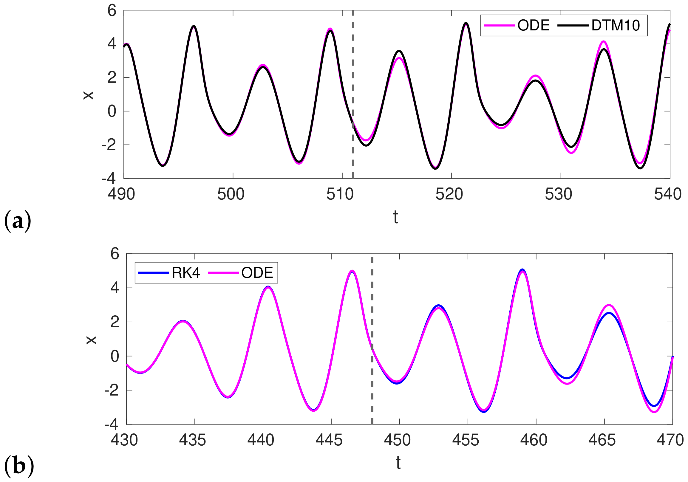
3.1. Integration of the Rössler System: DTM vs. Other Methods

To assess the quality of solutions obtained with the use of the DTM, a number of simulations of the chaotic Rössler system ($a=0.4079$) were performed, and their results were compared with results obtained with other methods. The Runge–Kutta 4 (RK4) scheme and the ode45 (ODE) Matlab solver with the sixth-stage fifth-order Runge–Kutta algorithm were implemented. The ode45 function is a versatile high quality function and it is recommended as the first solver to be tried in most problems. However, it has recently been reported [30] that the simple RK4 algorithm yields, in some cases, much better results than the latest Matlab ode functions. In the case of the ode45 function, an optional parameter was used to limit the maximum integration step ($h_{max}$). When assessing the quality of results obtained with various methods, we use the convergence criterion, the measure of which is the concurrency time of curves corresponding to two compared solutions. The best convergence of DTM and ODE results was found for the DTM order 10 with $h_{DTM}=0.01$ s and for $h_{max}=0.002$ (Figure 1a).

Figure 1. (a) Borderline of the convergence between ODE and DTM solutions with optimal parameters: DTM order equals 10, $h_{DTM}$ = 0.01 s and $h_{max}$ = 0.002 s. (b) Borderline of convergence between ODE and RK4 results. The time step adopted in the RK4 method was $h_{RK4}$ = 0.0002.

The duration of convergence between the ODE and RK4 results was 448 s (Figure 1b). Looking for the longest convergence times, a series of tests was carried out for different step lengths adopted for each method. The obtained results are presented in Figure 2.

Figure 2. (a) Duration of convergence between the DTM and optimal ODE ($h_{max}$ = 0.002 s). (b) Duration of convergence between the ODE and optimal DTM (order 10, $h_{DTM}$ = 0.01 s). (c) Duration of convergence between the RK4 and optimal ODE result. In all cases, the best results are marked with red points.

Figure 2a shows the duration of convergence between the DTM and ODE results when several DTM results obtained for different time steps are compared with the optimal ODE result. Results of the inverse comparison-ODE vs. DTM-are shown in Figure 2b. A comparison of the RK4 results with the optimal ODE result (Figure 2c) showed that the best time step was $h_{RK4}$ = 0.0002 s.

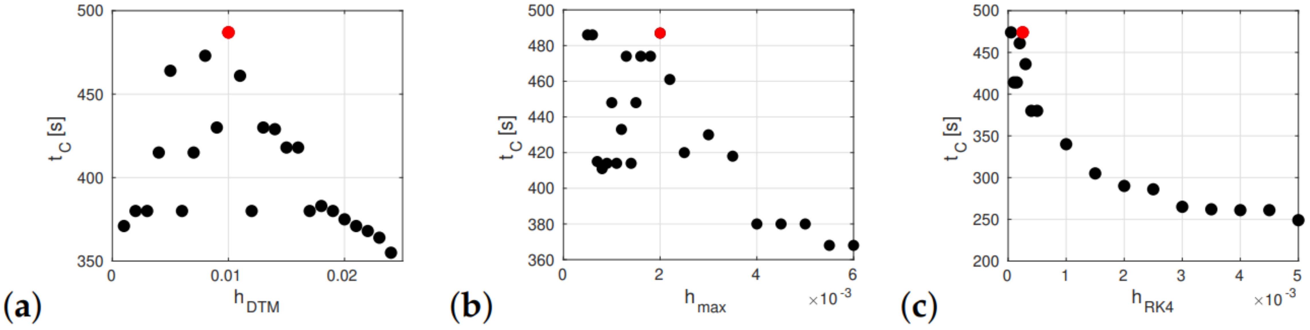
3.2. Finding the Optimal Order of DTM

The results discussed in Section 3.1 were obtained for the integer-order chaotic ($a=0.4079$) Rössler system. Since the chaoticity and fractionality of the system influence its dynamic characteristics, the optimal DTM order was determined separately for three cases: (a) an integer-order periodic (a = 0.4) system, (b) integer-order chaotic ($a=0.4079$) system, and (c) fractional-order ($\alpha =0.8$) chaotic ($a=0.4079$) system. The optimal order of the DTM was determined each time by obtaining convergence for solutions whose orders differed by 1. Taking into account the nonchaotic integer-order system, we noticed that, for the third-order solution (DTM-3), the results were almost identical to the DTM-4 results.

The DTM-4 and DTM-3 results are exactly the same in a 2D phase space (Figure 3b), but they differ in a 3D phase space (Figure 3c). This fact results from a phase difference between the two solutions (Figure 3a). Basically, the two results on the 3D plot match. In Figure 3b, we can only observe a local color change resulting from a different order of drawing the curves by the Matlab graphical function, which results from a phase difference between the two solutions. The phase difference occurs because DTM3 and DTM4 have different accuracies. As a result, their trajectories diverge and are attracted to the attractor at different locations of the phase space. For this case, a full agreement is obtained between the DTM-5 and DTM-6 results, which means that the optimal order of the DTM for integer-order periodic systems is 5. A comparison of different solutions of the integer-order chaotic Rössler system showed an exact convergence between the DTM-11 and DTM-12 results. Therefore, it can be claimed that the DTM order equal to 11 is optimal for this case. For the fractional and chaotic Rössler system, a total convergence was obtained between the DTM-14 and DTM-15 results. This proves that the greatest accuracy of solutions is generally obtained for the DTM order of 14. Despite the fact that the best solution of the chaotic fractional system is obtained for the DTM of order 14, the solutions of the lower orders are qualitatively similar to it.

Figure 3. (a) DTM3 vs. DTM4 for the periodic Rössler system of the integer order ($h_{DTM}$ = 0.01 s). Two identical results shifted in phase. (b) In a 2D phase space, the DTM3 result agrees with the DTM4 result. (c) In a 3D space, the phase shift makes a difference.

Figure 4a–c,f show the 2D phase diagrams of the results obtained by the DTM of the orders 2, 3, 5 and 10, respectively. Figure 4d,f compare the 3D phase diagrams of the DTM-10 result with DTM-2 and DTM-5, respectively. Despite the fact that the DTM-2 result in the 2D phase diagram (Figure 4a) differs from the DTM-10 result (Figure 4f), the shape of both attractors in the 3D phase diagram is similar (Figure 4d). In turn, a comparison of the DTM-5 and DTM-10 results reveals that they are similar both in the 2D (Figure 4c,f) and 3D (Figure 4e) phase diagrams.

Figure 4. Results obtained for the fractional chaotic Rössler system, $h_{DTM}$ = 0.01 s. Results in a two-dimensional phase space: (a) DTM of the second order, (b) DTM of the third order, (c) DTM of the fifth order, and (f) 10th order DTM. Results in a three-dimensional phase space: (d) comparison of DTM-2 and DTM-10 results, (e) comparison of DTM-5 and DTM-10 results.

All calculations presented in this paper were made in MATLAB, with an accuracy of 16 significant digits. While performing preliminary and actual test calculations, it was observed that changing one numerical formula to another (mathematically equivalent) would change the simulation results. This is the expected effect caused by different error propagation for different numerical formulas. This effect should be taken into account when comparing different calculation results obtained for the same parameters of the applied method. Convergence times in the cases being compared may not be fully consistent.

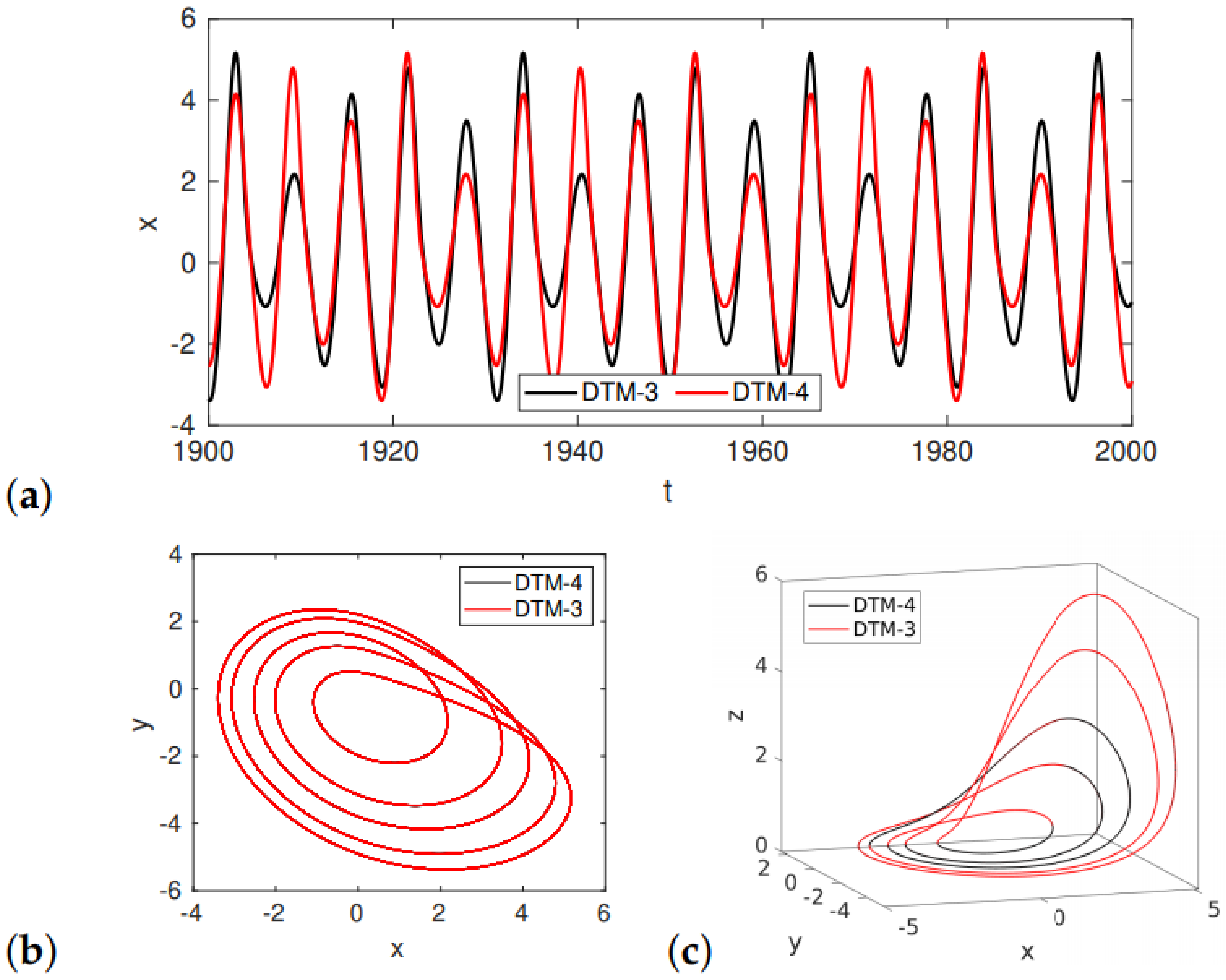
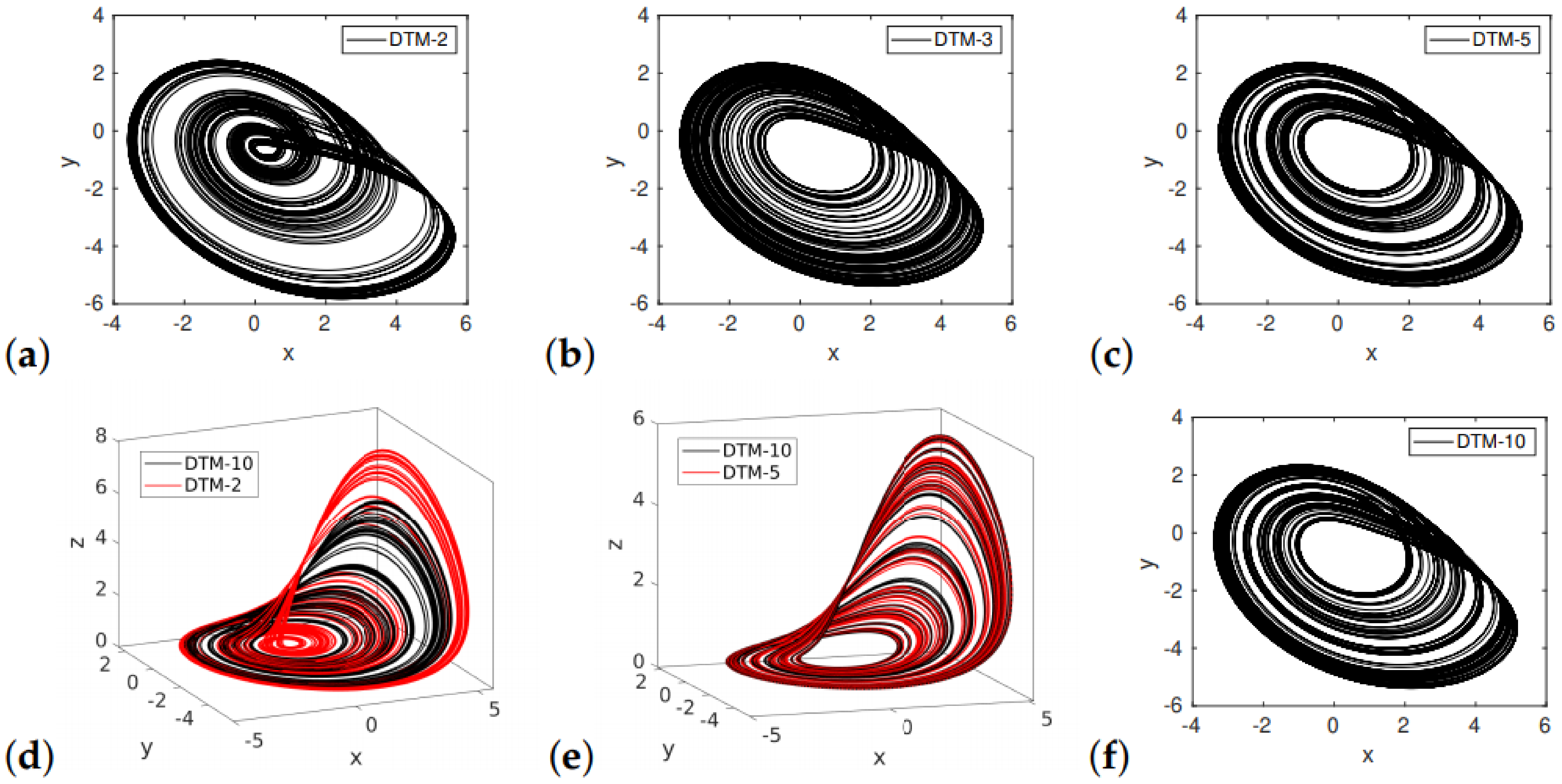
3.3. Integration of the Rössler System by DTM

In some studies on the DTM, one can find comparisons of results for different orders of the DTM or comparisons between the DTM and other integration schemes. Usually, these are results in the form of time series or phase diagrams that are compared. These comparisons are similar to those made in this study (Figure 1, Figure 3 and Figure 4) in order to determine the optimal parameters of the DTM for solving the Rössler system. The question remains, however, how the DTM solution of the Rössler system will be affected by changing the coefficients of the system (6). To assess this effect for the fractional system, a comparison is made between bifurcation diagrams that were determined using two integration methods: (a) a method based on the Grünwald–Letnikov definition of fractional derivative with the use of RK4 method (G-L RK4) and (b) the DTM. In the G-L RK4 method, the integration step was set to $h=0.001$ and 17,500 history points of the system (its previous states) were taken into account. For the DTM case, $h=0.01$ (i.e., the optimal h value detected in the preliminary tests) and orders of 8 and 14 were tested. The coefficient a was used as a bifurcation parameter. The system fractionality was induced by the fractional order of only the first equation (${\alpha }_1\ne 1$). The results obtained for ${\alpha }_1=0.98$ are presented in Figure 5 and for for ${\alpha }_1=0.96$ in Figure 6.

Figure 5. Bifurcation diagrams obtained for the Rössler system using two methods of integration: the RK4 scheme based on the Grünwald–Letnikov definition of fractional derivative and DTM for ${\alpha }_1=0.98$.

Figure 6. Bifurcation diagrams obtained for the Rössler system using the G-L RK4 scheme and DTM for ${\alpha }_1=0.96$.

The results shown in Figure 5 for the system with a relatively low fractionality are similar. One can only observe a slight shift to the right of the DTM result in relation to the G-L result, towards the positive values of the bifurcation parameter a. As the fractionality of the system increases ($\alpha =0.96$) (Figure 6), the result obtained by the G-L method changes qualitatively, while the overall characteristic of the DTM result remain unchanged. The shift of both results to the right increases. Based on these results and the results of previous tests, it can be concluded that the DTM results are more resistant to the change in the dynamics of a chaotic system. In the G-L RK4 method, the accumulation of errors in the iterative procedure quickly leads to qualitative changes in the obtained solutions. These changes depend on the dynamic characteristics of the system, i.e., on the value of the bifurcation parameter. As a consequence, when the fractionality of the system is changed, the bifurcation diagrams obtained by the G-L RK4 method are considerably modified while the DTM results are changed to an insignificant extent. Obviously, the DTM solution is not perfect; however, in the analyzed range of parameters, it is more resistant to iteration errors, which makes the obtained results more stable and thus resistant to changes in the system dynamics.

4. Conclusions

This study investigated the use of the multi-step differential transform method as a tool for integrating the classical autonomous Rössler system of a fractional order. In preliminary studies of the integer-order system, the quality of the DTM was assessed by comparing its results with those obtained with numerical tools widely used to integrate differential equations: the RK4 scheme and the Matlab ode45 function. The study has demonstrated that h = 0.01 is the optimal integration step value for the DTM. A comparison of different DTM cases for the chaotic fractional system with the adopted integration step of $h=0.01$ helps determine the optimal order of the method ($K=14$) which should be used in general. However, the same tests have shown that reducing the order to $K=8$ does not lead to significant changes in the results of integration. These conclusions have been confirmed by the results of the investigation of the Rössler fractional system carried out for a wide range of changes in the bifurcation parameter (coefficient a). It has been found that the DTM results are very stable and resistant to changes for the system fractionality, ranging from ${\alpha }_1=0.98$ to ${\alpha }_1=0.96$. The same changes produce clear qualitative changes in the results obtained with the G-L RK4 method, which seems to be primarily caused by more intensive error propagation.

As mentioned in the introduction, when considering topological conditions of a solution obtained via DTM processing of the FODE in the Caputo sense, we must take into account possible inaccuracies resulting from limiting the solution of a three-dimensional space. Therefore, more theoretical analyses and numerical experiments are needed to better assess which of the two integrating approaches of the fractional system under consideration gives results that are closer to true solutions.

References

- Hilfer, R. Applications of Fractional Calculus in Physics; World Scientific Publishing Company: Singapore, 2000. [Google Scholar]
- Kilbas, A.A.; Srivastava, H.M.; Trujillo, J.J. Theory and Applications of Fractional Differential Equations; North-Holland Mathematical Studies; Elsevier (North-Holland) Science Publishers: Amsterdam, The Netherlands, 2006; Volume 204. [Google Scholar]
- Jafari, H.; Daftardar-Cejji, V. Solving a system of nonlinear fractional differential equations using Adomian decomposition. J. Comput. Appl. Math. 2006, 196, 640–651. [Google Scholar] [CrossRef]
- He, J.-H. An elementary introduction to the homotopy perturbation method. Comput. Math. Appl. 2009, 57, 410–412. [Google Scholar] [CrossRef]
- Zayeranouri, M.; Matzavinos, A. Fractional Adams-Bashfort/Moultn methods: An application to the fractional Keller-Segel chemotaxis system. J. Comput. Phys. 2016, 317, 1–14. [Google Scholar] [CrossRef]
- Zhou, J.K. Differential Transformation and Its Applications for Electrical Circuits; Huazhong Univ. Press: Wuhan, China, 1986. [Google Scholar]
- Chen, C.K.; Ho, S.H. Solving Partial Differential Equations by Two-Dimensional Differential Transform Method. Appl. Math. Comput. 1999, 106, 171–179. [Google Scholar]
- Ertúrk, V.S.; Odibat, Z.M.; Momani, S. The Multi-Step Differential Transform Method and Its Application to Determine the Solutions of Non-Linear Oscillators. Adv. Appl. Math. Mech. 2012, 4, 428–438. [Google Scholar] [CrossRef]
- Mirzaee, F. Differential Transform Method for Solving Linear and Nonlinear Systems of Ordinary Differential Equations. Appl. Math. Sci. 2011, 70, 3465–3472. [Google Scholar]
- Odibat, Z. Generalized differential transform methodfor solving Volterra integral equation with separable kernels. Math. Comput. Model. 2008, 48, 1144–1146. [Google Scholar] [CrossRef]
- Arikoglu, A.; Ozkol, I. Solution of fractional differential Equations by using differential transform method. Chaos Solitons Fractals 2007, 34, 1473–1481. [Google Scholar] [CrossRef]
- Cong, N.D.; Tuan, H.T. Generation of Nonlocal Fractional Dynamical Systems by Fractional Differential Equations. J. Integral. Equat. Appl. 2017, 4, 585–607. [Google Scholar] [CrossRef]
- Kuznetsov, N.V.; Makaev, T.N.; Kuznetsov, O.A.; Kudryashova, E.V. The Lorenz system: Hidden boundary of practical stability and the Lyapunov dimension. Nonlinear Dyn. 2020, 102, 713–732. [Google Scholar] [CrossRef]
- Leonov, G.A.; Kuznetsov, N.V.; Makaev, T.N. Homoclinic orbits, and self-excited and hidden attractors in a Lorenz-like system describing convective fluid motion. Eur. Phys. L. Spec. Top. 2015, 224, 1421–1458. [Google Scholar] [CrossRef]
- Boichenko, V.A.; Leonov, G.A.; Reitmann, V. Dimension Theory for Ordinary Differential Equations; Teubner: Stuttgart, Germany, 2005. [Google Scholar]
- Ladyzhenskaya, O.A. Attractors for Semi-Groups and Evolution Equations; Cambridge University Press: Cambridge, UK, 1991. [Google Scholar]
- Doan, T.S.; Kloeden, P.E. Semi-Dynamical System Generated by Autonomous Caputo Fractional Differential Equations. Vietnam J. Math. 2021. [Google Scholar] [CrossRef]
- Caputo, M. Linear models of dissipation whose Q is almost frequency independent—II. J. R. Austral. Soc. 1967, 13, 529–539. [Google Scholar] [CrossRef]
- Rössler, O. An equation of continuous chaos. Phys. Lett. 1976, 5, 397–398. [Google Scholar] [CrossRef]
- Barrio, R.; Blesa, F.; Dena, A.; Serrano, S. Qualitative and numerical analysis of the Rössler model: Bifurcations of equilibria. Comput. Math. Appl. 2011, 62, 4140–4150. [Google Scholar] [CrossRef][Green Version]
- Sprot, J.C.; Li, C. Asymmetric Bistability in the Rössler system. Acta Phys. Polonica B 2011, 48, 97–107. [Google Scholar] [CrossRef]
- Cafagna, D.; Grassi, G. Hyperchaos in the Fractional-order Rössler System with Lowest-order. Int. J. Bifurc. Chaos 2009, 1, 339–349. [Google Scholar] [CrossRef]
- Wang, H.; He, S.; Sun, K. Complex Dynamics of the Fractional-Order Rössler System and Its Tracking Synchronization Control. Complexity 2016. [Google Scholar] [CrossRef]
- Zhang, W.; Zhou, S.; Li, H.; Zhu, H. Chaos in a fractional-order Rössler system. Chaos Solitons Fractals 2009, 42, 1684–1691. [Google Scholar] [CrossRef]
- Freihat, A.; Momani, S. Adaptation of Differential Transform Method for the Numeric-Analytic Solution of Fractional-order Rössler Chaotic and Hyperchaotic Systems. In Abstract and Applied Analysis; Hindawi: London, UK, 2012. [Google Scholar]
- Idrees, M.; Mabood, F.; Ali, S.; Zaman, G. Exact Solution of Stiff System by Differential Transform Method. Appl. Math. 2013, 4, 440–444. [Google Scholar] [CrossRef]
- Odibat, Z.; Momani, S.; Ertúrk, V.S. Generalized differential transform method: Application to differential equations of fractional order. Appl. Math. Comput. 2008, 197, 467–477. [Google Scholar] [CrossRef]
- Alomari, A.K. A new analytic solution for fractional chaotic dynamical system using the differential transform method. Comput. Math. Appl. 2011, 61, 2528–2534. [Google Scholar] [CrossRef]
- Odibat, Z.; Bertelle, C.; Aziz-Alaoui, M.A.; Duchamp, G. A multi-step differential transform method and application to non-chaotic and chaotic systems. Comput. Math. Appl. 2010, 59, 1462–1472. [Google Scholar] [CrossRef]
- Keevil, J. ODE4 Gives More Accurate Results than ODE45, ODE23, ODE23s. MATLAB Central File Exchange. Available online: https://www.mathworks.com/matlabcentral/fileexchange/59044-ode4-gives-more-accurate-results-than-ode45-ode23-ode23s (accessed on 20 July 2021).
Publisher’s Note: MDPI stays neutral with regard to jurisdictional claims in published maps and institutional affiliations. |
© 2021 by the authors. Licensee MDPI, Basel, Switzerland. This article is an open access article distributed under the terms and conditions of the Creative Commons Attribution (CC BY) license (https://creativecommons.org/licenses/by/4.0/).