Article

Scalability of Water Property Measurements in Space and Time on a Brackish Archipelago Coast

Department of Geography and Geology, University of Turku, FI-20014 Turku, Finland
*
Author to whom correspondence should be addressed.
Appl. Sci. 2021, 11(15), 6822; https://doi.org/10.3390/app11156822
Submission received: 15 June 2021 / Revised: 19 July 2021 / Accepted: 22 July 2021 / Published: 24 July 2021
(This article belongs to the Special Issue Applied Geoinformatics: From Coastal to Fluvial Geography)

Abstract

:
Our paper aims at advancing global change management in marine archipelago environments. Water properties vary along temporal and vertical gradients, and studies indicate that these patterns may be site-specific, i.e., they may vary at local or regional scales. Understanding these complex processes is crucial for designing environmental monitoring campaigns or assessing the scalability of their results. To our knowledge, the four-dimensional (temporal, vertical and horizontal) patterns of water quality have not been statistically quantified. In this paper, we partition the variation in four key water property variables into temporal, vertical and horizontal dimensions, by utilising a unique pre-existing high-density dataset and multilevel regression modelling. The dataset comprised measurements of temperature, salinity, pH and chlorophyll-a concentration, sampled eight times from April to October on the SW Finnish archipelago coast. All variables were sampled along the depth gradient and at local (102 m) and regional scales (104 m) at 20 sites. All measured variables varied significantly along the temporal and vertical gradients, and the overall levels, temporal patterns and vertical gradients of these variables were significantly site-dependent. Our study confirms that many water properties, especially chlorophyll-a concentration, show high four-dimensional variability in the complex archipelago environment. Thus, studies on the regional dynamics of archipelago water properties call for a high sampling density in time, along the vertical gradient, and in space.

1. Introduction

Coastal waters form a globally important environment at the land–sea interface, where the aquatic ecosystems are diverse, and the human influence on the sea is at its highest. Particularly in estuaries and other semi-enclosed coastal areas, the brackish water zone is often a very complex marine environment where the physicochemical processes, water flows and ecological features form dynamic and detailed patterns. However, understanding the patterns and processes of these environments is crucially important when trying to maintain and improve their ecological status, and to prepare for the impacts of global change [1,2,3,4]. A better understanding of the current status and the processes is needed to improve the science-based management of the marine archipelago environments in the future [5,6,7,8].
Coastal waters are typically complex and gradually shifting zones between the mainland shoreline and the pelagic realm. Within this zone, high local variability and temporal inconsistency in water properties often occur [9,10,11,12,13,14,15], and the variation is usually different among the parameters. When monitoring the status of the coastal marine environment and the impacts of nature conservation measures, the sampling must be carefully fitted to the spatial and temporal scales of the phenomena [9,16], since the results of a monitoring campaign are highly sensitive to the timing and location of the sampling [17,18,19,20].
Archipelago coasts, in particular, are characterised by a notable spatial and temporal variation in water properties [9,10,
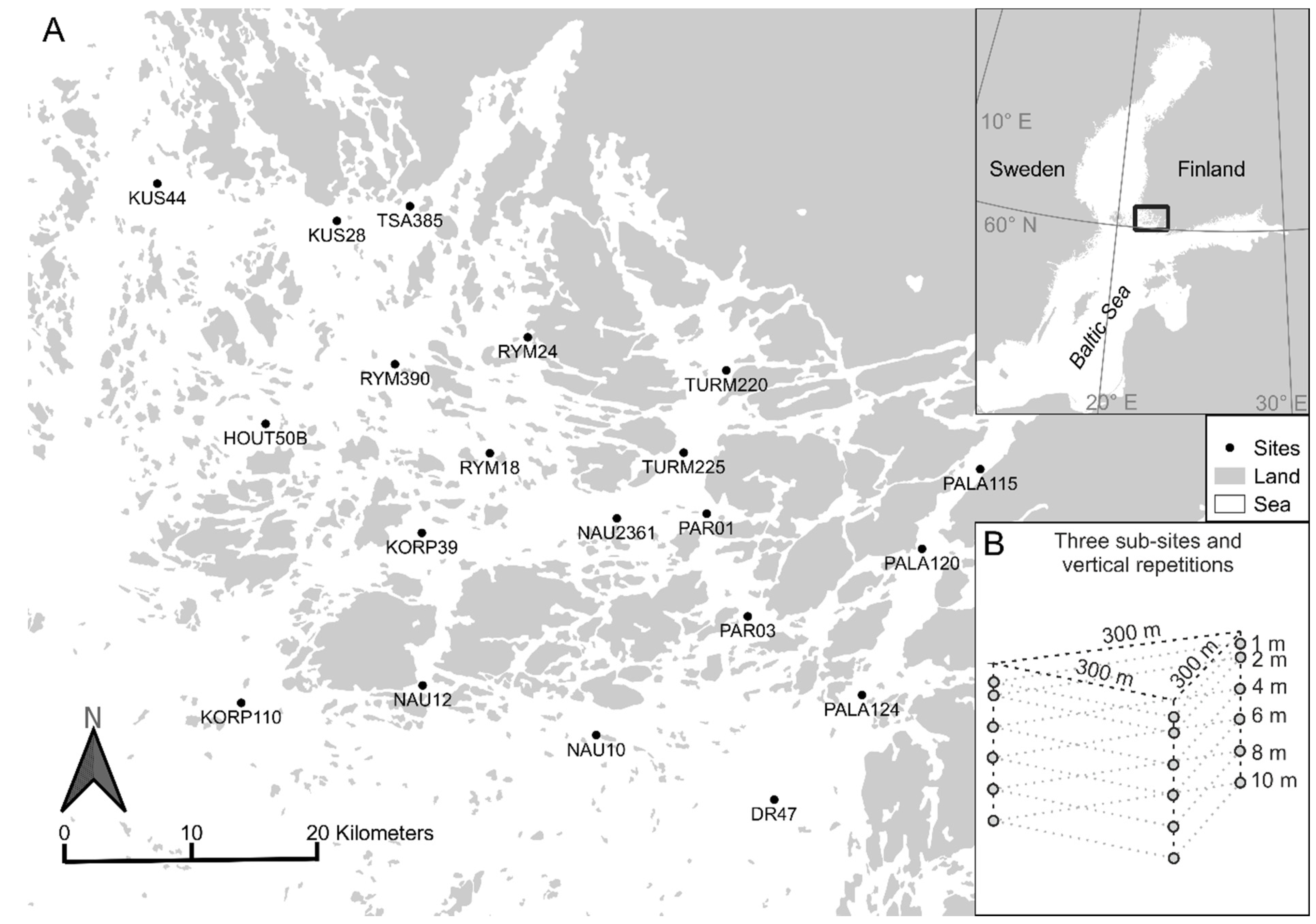
21]. Our study area, the SW Finnish archipelago coast in the Baltic Sea, is a good example, where small and large islands, deep basins, shallows and sills create a very complex bathymetry [9]. The varying bathymetry causes restrictions in water exchange [22]. In addition, the location of many archipelagos at the land–sea-interface causes local and temporal variation in marine and terrestrial influences [23]. For example, a large component of the variability in water properties in the SW Finnish archipelago is persistent and depends on the location along the land–sea transition: Suominen et al. [9] reported clear spatial trends in the water properties along the mainland–open sea axis.
Seasonality causes an important component of variability in water properties in higher latitudes. This includes a high annual temperature and stratification cyclicity, winter ice cover, and high variability in runoff due to snow accumulation and melting. Thus, in addition to the spatial complexity, the temporal complexity is distinct. These complexities together make brackish coastal archipelagos, such as the SW Finnish coast, very dynamic and challenging to monitor. The environmental conditions vary due to the presence of islands and shallow topography, causing the seasonal developments (i.e., timing and magnitude) of, e.g., algal growth, to differ within small areas—numerous previous studies, which have utilised in situ and remotely sensed data and spatial modelling, highlight these features in the SW Finnish archipelago in terms of spatial [11,24,25], temporal [9,12,26], and spatio-temporal variability [10,27]. Many studies conclude that the variation is difficult to capture, and it is advisable to use combined methods to complement in situ sampling (e.g., [9,10,11,12,26]). However, to our knowledge, the four-dimensional (temporal, vertical and horizontal) patterns of water quality have not yet been statistically quantified.
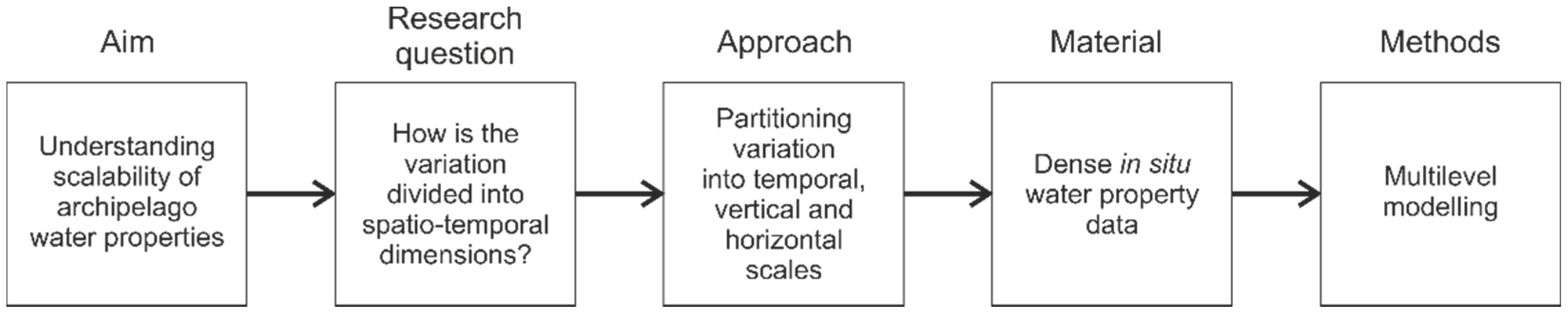
This study aimed at statistically examining the scalability of water properties in space and time in a heterogeneous archipelago (Figure 1). More specifically, we examined how the variation in archipelago water properties is divided into the temporal, vertical and horizontal dimensions (Figure 1). We pursued this by statistically reanalysing a unique, pre-existing dataset from the SW Finnish archipelago (described in Suominen et al. [9]). This dataset included four water property variables: temperature, salinity, pH and chlorophyll-a concentration. The measurements were repeated densely at local (102 m or hundreds of metres) and regional (104 m or tens of kilometres) scales, along the vertical gradient (topmost 10 m) and in time (three-week intervals) during one growing season (May–October). We partitioned the variation in water properties to temporal, vertical and spatial dimensions utilising multilevel modelling, to gain better understanding of the scalability of the in situ measurements of different water parameters on the archipelago coast (Figure 1).

2. Materials and Methods

2.1. Study Area

The analyses were based on a pre-existing dataset from the SW Finnish archipelago [9]. The study covered an area of c. 2500 km2, and it was c. 50 km and 70 km wide in the west–east and south–north directions, respectively. The study area was located in the northern limits of the temperate zone at 60° north, within the semi-enclosed Baltic Sea basin. The summer peak in primary production takes place typically in July and August.
The area provided a good test case for the analysis, since it is very complex: it is shallow (0–100 m), has c. 25,000 islands (counting those with an area over 500 m2), is geologically and bathymetrically varying and exhibits a strong land–sea transition. The area is further characterised by brackish water (salinity varying between 0 and 7‰ in this area along the land–sea-continuum [13,28]), and seasonal sea ice cover (up to 100 days annually [29]). The SW Finnish archipelago has a clear seasonal cycle in physicochemical processes: a stratification develops in the summer and in the winter and is interrupted by vertical autumn and spring circulations. Moreover, there are very high concentrations of organic dissolved matter [30], and the archipelago is therefore highly eutrophic [31,32].

2.2. In Situ Data

The analyses were based on a pre-existing dataset from 2007, described in Suominen et al. [9]. This dataset was found to be suitable for our purpose since it included spatially dense and frequent in situ measurements of water properties in the topmost water column during one growing season. Water properties were measured in situ from week number 20 in mid-May to week number 40 in early October 2007. Weather and sea ice conditions during this period were in the normal range compared to long-term averages.
The sampling was carried out on eight occasions, approximately every three weeks. This sampling frequency allowed us to examine the variation in water properties caused by the algal growth cycles [9]. Inside the study area, a network of 20 sampling sites was established (representing the regional scale (104 m); Figure 2). The selected sites were extracted from the national monitoring network (published by the Finnish Environment Institute SYKE), hence their nomenclature. The site “NAU2361” in the centre of the study area (Figure 2) is monitored by the national authorities continuously, the other 19 sites sparsely and irregularly.
At each site, three sub-sites with 300 m distances from each other were measured each time (representing the local scale 102 m; Figure 2). In addition, measurements were repeated at all sub-sites at six depths: 1, 2, 4, 6, 8 and 10 m below the surface (Figure 2). The dataset thus had a three-dimensional statistical structure (space, time, depth) and the spatial dimension had a two-level nested structure (Table 1). The nested structure of the data was in principle balanced, with almost all sites (18 out of 20) and sub-sites (54 out of 60) having an equal number of observations (Table 1). The few missing observations were caused by harsh weather conditions [9].
Coordinates were recorded at each sub-site during each field visit. The following water property variables were measured in situ with a YSI 6600 V2 multiparameter sonde (YSI Inc., Yellow Springs, OH, USA) at each depth (Table 2): temperature and salinity (specific conductance; sensor YSI 6560), pH (sensor YSI 6565) and chlorophyll-a (relative fluorescence units, RFU; sensor YSI 6025). The in situ measurements were compared to water samples in a certified laboratory setting (laboratory of the Water Protection Association of Southwest Finland). The calibration, validation and variable transformation procedures were described in detail by Suominen et al. [9].

2.3. Statistical Analyses

We performed multivariate regression modelling to partition variation in the four response variables, water temperature, salinity, pH and chlorophyll-a concentration (Table 2), into temporal and vertical dimensions. In practice, we examined the statistical relationship between the response variables and two predictor variables, week and depth (Table 1). Multilevel modelling was applied to examine the site- and sub-site-level variability in water properties.
First, we partitioned variation in the four water property variables into temporal and vertical dimensions, by identifying the significance of “week” and “depth” terms in the multivariate regression model. We accounted for the general vertical and seasonal patterns of water properties of the SW Finnish archipelago by looking for the best linear regression model structure. We fitted multivariate linear regression models to the water property data, using a combination of backward and forward stepwise regression to identify the best model variant for each water property variable. These models are hereafter called “observation-level models” for comparison to multilevel models. We considered linear and higher-order (up to 10th order) terms of “week” and “depth” and the first-order interaction term (“Week:Depth”) in the models (Equation (1)). Considering high-order models allowed us to find well-fitting multivariate models that account for complex seasonal cycles in water properties. This ensured that all unexplained variance is due to factors other than time and depth, and thus facilitated the examination of site- and sub-site-specific patterns in the following modelling steps. The predictors were standardised, i.e., centred and scaled, before analysis to reduce convergence and collinearity issues [32,33].
Response ~ Week + Depth + Week2 + Depth2 …. + Week10 + Depth10 + Week:Depth
Individual terms were sequentially dropped in the order of their t-statistic, and the performance of model variants was examined based on the Bayesian information criterion (BIC).
Second, we examined the general variation of the four water property variables along temporal and vertical gradients. After the identification of the best observation-level model variant, the interactive effects of “week” and “depth” on each water property variable were examined [34] by plotting the back-transformed effect of “week” on the water property variable at different depths.
Third, we partitioned the variation in the four water property variables into horizontal scales (local and regional). We examined water property variation at the site and sub-site levels by fitting simple linear multilevel models, or intercept-only models, to the water property data. The more complex intercept-only models (Equation (2)) included nested random intercepts for the site and sub-site structures:
Response ~ (1|Site/Sub-site)
A simpler variant of the intercept-only multilevel model included a random intercept for site (Equation (3)). Thus, the intercept-only models allowed the overall level of the water property variable to vary between spatial locations.
Response ~ (1|Site) (or Yij = γ00 + u0j + eij)
where Yij = the ith observation in the jth group, γ00 = the overall mean, u0j = group-level residuals, and eij = observation-level residuals (residual error). We calculated intraclass correlation (ρ; Equation (4)) for these intercept-only models, to quantify the proportion of the variance explained by the spatial grouping structure in the observations. Thus, intraclass correlation examined how much of the variation in one water property variable depended on location.
ρ = σ²u0/(σ²u0 + σ²e)
where σ2u0 = variance of the group-level residuals u0j, and σ2e = variance of the observation-level residuals eij [33]. Since no variance was found at the sub-site level, the following procedures are described for the simpler site-level models only.
Fourth, we examined the interaction of temporal and vertical gradients of the four water quality variables with spatial location. In other words, we examined how the temporal and vertical gradients vary between sites and sub-sites. We partitioned the variation in water property variables to temporal (week), vertical (depth) and horizontal (site) scales by fitting full multilevel models. The multilevel models were fitted using the restricted maximum likelihood method (REML). These models combined observation-level terms of explanatory variables with random intercepts (Equation (2) or (3)) and random slopes for “week” and “depth”.
The multilevel models were fitted sequentially (following [33]) to examine the contribution of each term to the BIC and residual variance. The sequential fitting started from random intercept models, including observation-level terms and nested random intercepts for “site” and “sub-site”:
Response ~ Week + Depth + Week2 + Depth2 … + Week10 + Depth10 + Week:Depth + (1|Site/Sub-site)
Finally, random slope models were fitted, including site-level random terms for the first- and second-order terms of the explanatory variables:
Response ~ Week + Depth + Week2 + Depth2 … + Week10 + Depth10 + Week:Depth + (1 + Week + Week2 + Depth + Depth2|Site)
The random structure of the multilevel model thus allowed both the intercept and slope coefficients of all fixed terms to vary between sites. Stepwise regression was again applied to identify an “optimal” model structure, with the lowest BIC (Appendix A).
All statistical analyses and modelling were performed with the R statistical software (version 4.0.3; [35]). Linear mixed models were fitted with the package lme4 (1.1–26; [36]) and examined with package lmerTest (3.1–3; [37]). The effects of the explanatory variables were calculated with package effects (4.2–0; [34]). The main and interactive effects of “week” and “depth” were calculated with the effect function by absorbing the lower-order terms marginal to the higher-order term in question and averaging over other model terms [38]. As a result, a table of predicted values at different levels of the two interacting factors was calculated. The package ggeffects (1.1.0; [39]) was utilised to calculate random effects for visualisation. Maps were created in QGIS (3.16; [40]) and all visualisations were finalised in R with packages ggplot2 (3.3.3; [41]) and gridExtra (2.3; [42]).

3. Results

3.1. General Vertical and Seasonal Patterns in Water Properties

Based on the BIC, the best models for all four response variables had similar base structures (Table 3). All models included “week” and “depth” as predictors, the interaction term between “week” and “depth” and up to seventh-order polynomials for “week” (Table 3). Only the chlorophyll-a model included a higher-order (second-order) term for “depth”. The selection of terms included in the models remained identical throughout the modelling steps, i.e., in the observation-level, random intercept, and random slope models. In addition, the estimated coefficients of the predictor terms remained almost identical throughout the modelling process (Table 3). These results indicated that the estimated fixed effects were robust: the identified relationships were not sensitive to the selection of the modelling method.
The estimated model coefficients showed considerable variation between response variables (Table 3). Thus, the fitted models indicated that the four response variables had different relationships with time and depth. Temperature showed a unimodal relationship with time, peaking during week 34 in late August (Figure 3A). The linear drop of temperature with depth decreased and finally disappeared with time (Figure 3A). Salinity increased during the study period, and the slight layering (least saline water at the top) decreased and disappeared with time (Figure 3B). pH generally decreased with time, with the largest changes at the beginning of the period (Figure 3C). The layering in pH decreased slightly with time (Figure 3C).
The temporal changes in the chlorophyll-a concentration were most complex. Chlorophyll-a reached its minimum during week 23 (early June) and peak during weeks 31–34 (August; Figure 3D). The vertical pattern in chlorophyll-a turned over during the period: the topmost layer had the lowest concentration in early spring but the largest concentration in late autumn (Figure 3D). Based on the model, the layering was strongest at the end of the period (Figure 3D).

3.2. Variability of Water Properties at Site and Sub-Site Levels

For temperature, intraclass correlation for site in the intercept-only model was 0.01 (Table 4). This indicated that only 1% of the variance in temperature was at the site level. However, the intraclass correlations for other response variables suggested that 34, 12 and 17% of variation was at the site level for salinity, pH, and chlorophyll-a, respectively (Table 4). This meant that the overall level of these three variables differed notably between sites. Intraclass correlation for the nested site–sub-site structure was zero across all models (Table 4). This means that there was no significant variance at the sub-site level. Therefore, an appropriate random model structure included random effects only for site. Even though the ICC for temperature was low, a mixed-effects model appropriately dealt with the nested data structure and was therefore also seen as the best model structure for temperature.

3.3. Variability of Temporal and Vertical Patterns at Regional and Local Scales

Sequential fitting of the random slope models and examination of the BIC indicated that the best multilevel models for all four water property variables included random slopes for the first- and second-order “week” terms (Table 5). In addition, all models included a random slope for “depth” (Table 5). Thus, the best-performing multilevel models allowed the intercept and slope coefficients for both “week” and “depth” to vary between sites.
In practice, the random intercept allowed the overall level of the response variable to vary between sites, thus reflecting real-life differences in the level of a water property variable. The random slope coefficient for “week” meant that the value of each water property variable changed more rapidly with time in specific sites than in others. Similarly, the random slope coefficients for “depth” indicated that the strength of the vertical water property gradients varied between sites.
The best multilevel models succeeded in explaining 95%, 92%, 79% and 60% of variance in temperature, salinity, pH and chlorophyll-a, respectively (Table 6). The improvement of model performance, compared to the corresponding observation-level model, was notable for salinity (Figure 4), pH and chlorophyll-a, since the models were able to accommodate site-specific relationships between water properties, time and depth. For example, compared to linear regression models, the best multilevel model for salinity decreased residual variance from 0.46 to 0.08 (Table 6; Figure 4). Overall, the chlorophyll-a models performed worst, but the improvement in performance compared to observation-level models was notable (decrease in residual variance from 0.72 to 0.40; Table 6). For temperature, the performance of the best observation-level model was so high that there was little room for improvement in multilevel models (Table 6).
The random slope models for salinity (Figure 5) and chlorophyll-a (Figure 6) indicated the most distinct random effects, i.e., the largest site-specific variation in the overall levels and in the temporal and vertical patterns. For example, salinity was generally highest (highest intercept) in the southern sites in the outer archipelago and lowest in the inner archipelago (e.g., KORP110 and TSA385, respectively; Figure 5). The slope of the first-order “week” term was generally steepest in the north-western part of the study area, meaning that the increase in salinity during the summer season was most distinct (Figure 5). In some other sites, such as “PAR01”, salinity did not exhibit a clear increasing trend (Figure 5).
The overall level (intercept) of chlorophyll-a was highest in the central inner archipelago, as well as in the southern sites (Figure 6). The random effects indicated very different and even opposite temporal changes in chlorophyll-a concentration in the archipelago (Figure 6). For example, the model predicted the chlorophyll-a concentration to remain relatively low throughout the summer season in “KUS44” (Figure 6). However, increasing trends, decreasing trends and a high peak in the middle of the summer season were predicted by the same random slope model in sites “TSA385”, “PALA115” and “TURM220”, respectively (Figure 6).
The results of multilevel modelling indicated that, in the summer season of 2007, all four water quality variables varied significantly at the temporal and vertical scales (Table 7). In addition, all except temperature varied significantly at the regional scale and experienced site-specific temporal changes (Table 7).

4. Discussion

We present a detailed examination of the variation of key water properties in horizontal, vertical and temporal dimensions on a brackish archipelago coast, based on a unique high-density dataset. Our results demonstrate that the four water properties, temperature, salinity, pH and chlorophyll-a concentration, vary significantly at temporal and vertical scales. This alone confirms that the spatio-temporal variation of water properties in a complex coastal archipelago cannot be captured by temporally and vertically sparse sampling, as also suggested by previous studies (e.g., [9,10]). Further, the impact of time on water properties varies notably and somewhat predictably along the vertical gradient.
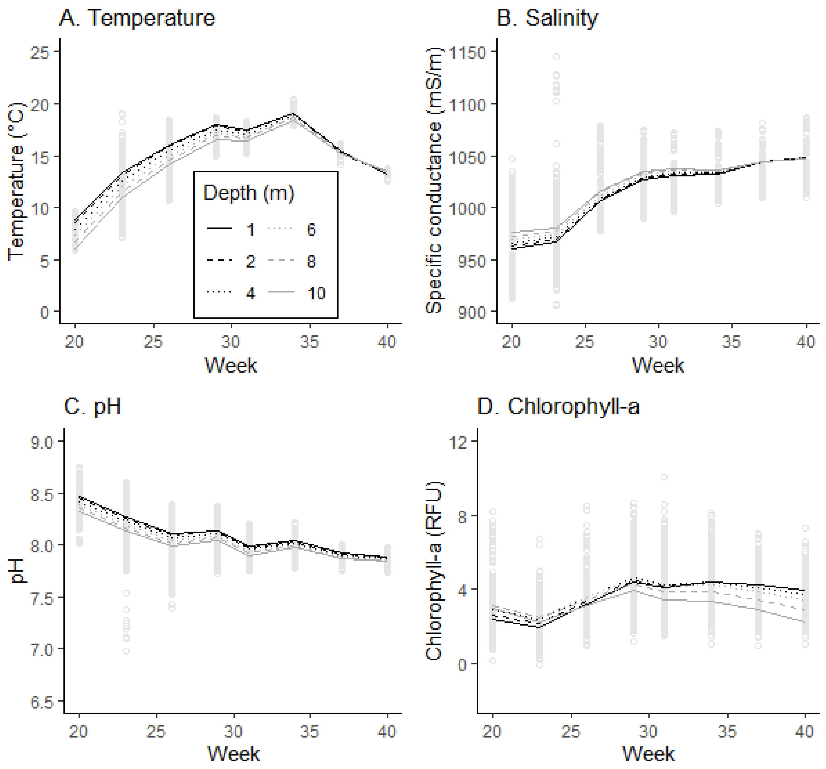
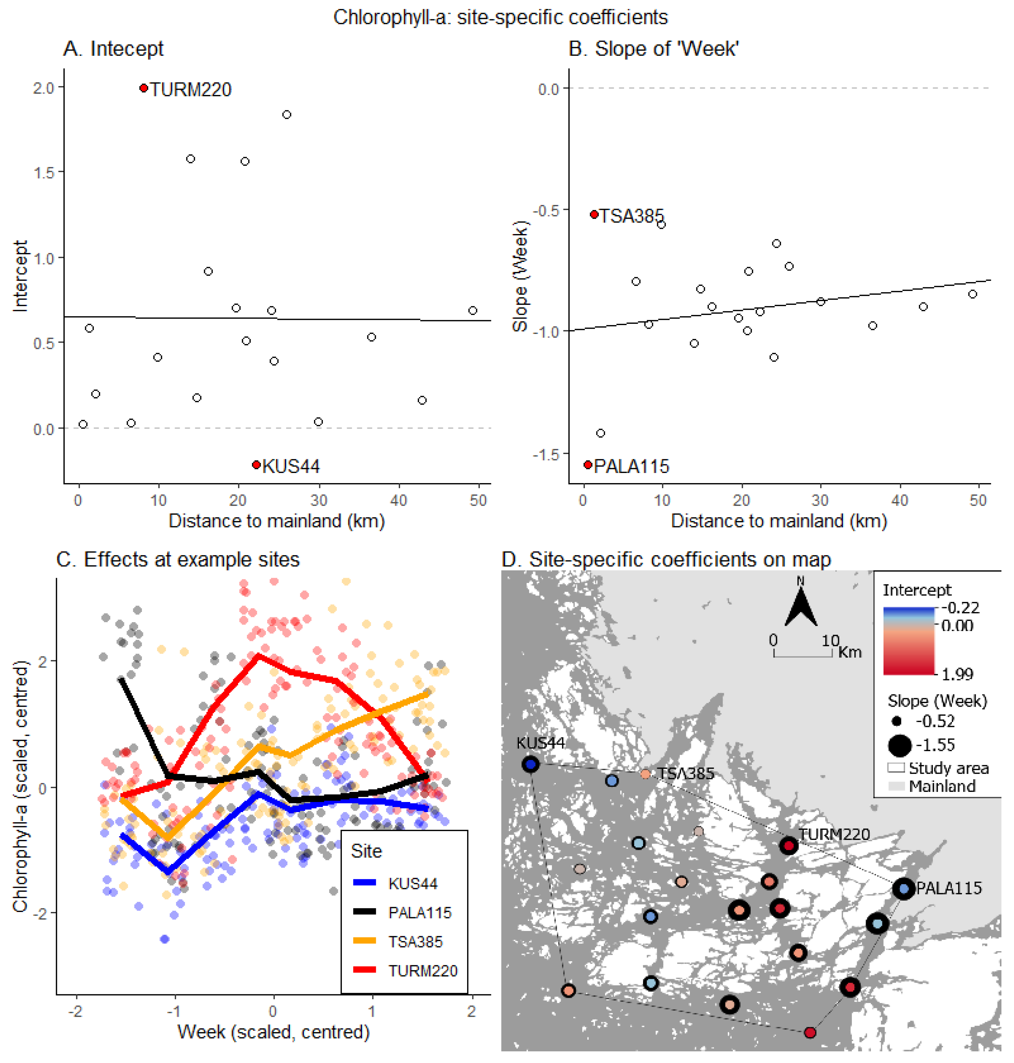
Chlorophyll-a exhibits the most complex temporal and vertical patterns, including a vertical shift of the chlorophyll-a concentration (Figure 3D and Figure 6C). In the spring, the lowest values are measured close to the surface, and highest values at the 10 m depth, while the situation is reversed in the autumn (Figure 3D). This indicates that there are different vertical distributions of the life cycles between the phytoplankton species occurring in the spring and in the later summer (e.g., [43,44]). The model captures the spring and later summer peaks in algal growth [
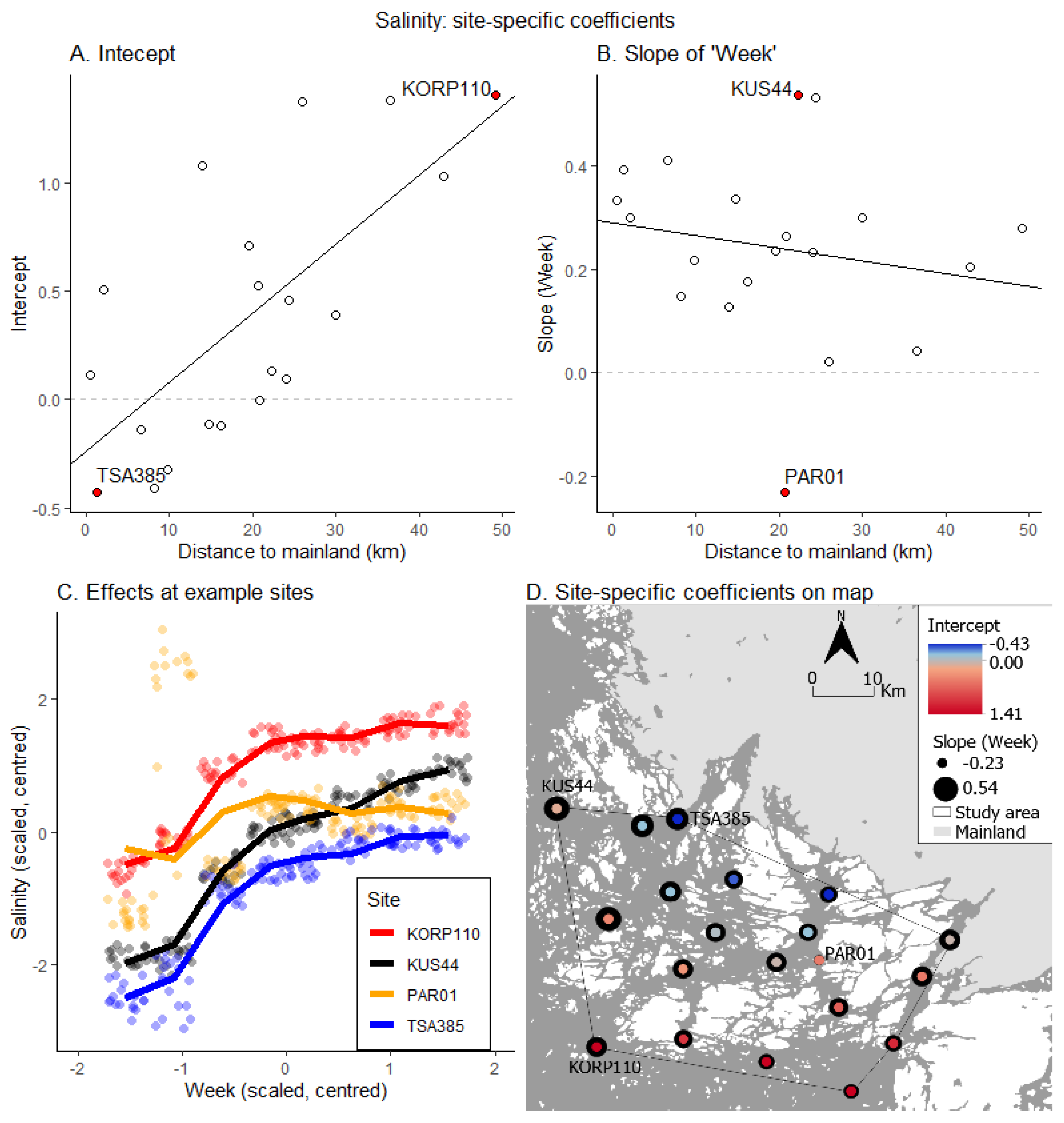
45], as well as a continuous increase in salinity throughout the study period.
A notable part of the variation in salinity, pH and chlorophyll-a occurs at the site level (12–34%), i.e., between locations that are several kilometres apart. Thus, salinity, pH and chlorophyll-a vary notably at the regional scale (104 m). Temperature varies more homogeneously at the regional scale, but finer details of the temporal–vertical patterns are site-dependant. No notable variance remains at the sub-site level. In other words, there is no local-scale (102 m) variation in water properties (Table 5). These findings statistically confirm the indicative results by Suominen et al. [9].
Instead of trying to explain why the variation among the water properties occurs, the aim of this study is to portray how the variation occurs spatio-temporally, and how it is divided into the horizontal, vertical and temporal dimensions. There are many underlying phenomena and measurable variables, such as nutrient concentrations, which regulate the chlorophyll concentration and the seasonal distribution of solar radiation, which regulates, among other things, the water temperature [46]. Instead of coupling the drivers with outcomes, this study confirms the significance of the water property variation in all dimensions.
Multilevel modelling proves to be an appropriate statistical approach to partitioning variation in water property variables into temporal, vertical and horizontal dimensions and examining their temporal and vertical gradients in different areas. As they are designed for accounting for the spatially nested structure of observations, they would be suitable for testing hypotheses on the drivers of water properties based on such spatial data. This is because the underlying assumption of independence in observation-level modelling (standard linear regression) is not fulfilled in spatially clustered data [33]. This is the case even if there is no significant variation between groups of observations, in this case between the sampling sites [33]. In addition, after incorporating suitable regional-level predictor variables into the models, they would be suitable for predictive water property modelling.
The results from our multilevel modelling suggest that both the overall level and the seasonal development of water properties vary at the regional (but not local) scale. In multilevel modelling, allowing the regression coefficients to vary between sites reveals important processes, which may be masked in observation-level examination. For example, only the best multilevel model for temperature allows the effect of depth to vary between sites, revealing potentially important vertical–temporal processes. Conversely, the depth profiles of salinity, pH and chlorophyll-a are similar among the sites.
Preliminary tests using second- and third-order models perform reasonably well for temperature, salinity and pH, and capture the main seasonal trends (see Appendix B). The more complex models (including up to seventh-order terms) are able to also capture the smaller temporal fluctuations in water properties. These preliminary findings suggest that the simpler second- and third-order models could be more suitable starting points for the predictive modelling of water properties (temperature, salinity and pH), i.e., when transferring the results into other areas and other years. The higher-order models seem to capture small-scale temporal variability of the particular observation period. These are potentially influenced by factors such as weather conditions and hydrological and oceanographic conditions.
It should be noted that national monitoring programs are designed to provide an overview of entire sea areas, and therefore they should not be expected to reveal regional-scale details. However, for example, the Finnish national program covers two (temporal and vertical) of the three relevant dimensions identified in this study: a small number of key sites (NAU2361 in our study area; see Figure 1) are sampled frequently throughout the year, and along the depth gradient. In addition, the Finnish national program has been running uninterrupted for decades, thereby offering long time-series data that enable inter-annual comparisons. Regarding regional-scale spatial detail, our results indicate that a single sampling site does not reliably represent water properties—apart from temperature—in the entire archipelago, not even at the nearest sites included in the national monitoring network. Thus, the temporally frequent sampling at one site only represents the very local (102 m) surroundings at the site. In addition, national monitoring programs may involve a spatially dense but temporally sparse sampling of water properties, such as in Finland. The results of one spatially dense sample cannot be generalised to other periods of time, since the seasonal development patterns are dissimilar among the sites.
The data and methodology used in this study provide solid statistical evidence on the issue of horizontal, vertical and temporal scalability of water property measurements. The methods are applicable in coastal areas anywhere to locally examine the scalability of in situ sampling. The predictability of water properties in other years based on the multivariate models for a single year is somewhat restricted, due to year-to-year variability in weather conditions and in the Atlantic forcing. To a degree, it can be assumed that the main spatio-temporal trends persist from year to year, but the lack of detailed data for other growing seasons sets a limitation to these conclusions. Further research on this topic would benefit from multi-annual in situ time series data from a few selected sites, as well as combining high-quality remotely sensed data to in situ data [47,48,49,50].

5. Conclusions

Our study confirms that the variation in archipelago water properties of temperature, salinity, pH and chlorophyll-a concentration is significant along the temporal and vertical (depth) gradients. All water properties except temperature vary significantly horizontally at the regional scale, but temperature conditions are more uniform. We also conclude that the seasonal developments and vertical profiles of these water properties are significantly different among nearby sites no more than 10 km apart in the Finnish Archipelago Sea, and that local-scale (102 m) variation is not an issue in the sampling of water properties. These findings have implications for designing environmental monitoring campaigns or assessing the scalability of their results, when managing global change in marine archipelago environments.

Author Contributions

Conceptualisation, T.N., H.T. and T.S.; methodology, T.N.; validation, T.N.; formal analysis, T.N.; investigation, H.T. and T.S.; data curation, T.N. and T.S.; writing—original draft preparation, T.N. and H.T.; writing—review and editing, T.N., H.T. and T.S.; visualisation, T.N. All authors have read and agreed to the published version of the manuscript.

Funding

This research received no external funding.

Institutional Review Board Statement

Not applicable.

Informed Consent Statement

Not applicable.

Data Availability Statement

The data presented in this study are available on request from the corresponding author. The data are not publicly available at the time of the submission of this paper due to ongoing further analyses.

Conflicts of Interest

The authors declare no conflict of interest.

Appendix A

Table A1. Stepwise observation-level regression results for the four response variables: BIC of each model variant after elimination of one term.
TemperatureBICSalinityBICpHBICChlorophyll-aBIC
Full817Full6006Full6123Full7296
[- Depth10]817[- Depth10]6006[- Depth10]6123[- Depth10]7296
[- Week10]817[- Week10]6006[- Week10]6123[- Week10]7296
[- Depth9]817[- Depth9]6006[- Depth9]6123[- Depth9]7296
[- Week9]817[- Week9]6006[- Week9]6123[- Week9]7296
[- Depth8]817[- Depth8]6006[- Depth8]6123[- Depth8]7296
[- Week8]817[- Week8]6006[- Week8]6123[- Week8]7296
[- Depth7]817[- Depth7]6006[- Depth7]6123[- Depth7]7296
[- Depth6]817[- Depth6]6006[- Depth6]6123[- Depth6]7296
[- Depth3]810[- Depth3]5998[- Depth3]6115[- Week6]7288
[- Depth5]802[- Depth5]5990[- Depth4]6107[- Depth4]7280
[- Depth4]795[- Week6]5982[- Depth5]6099[- Depth5]7273
[- Depth2]789[- Depth4]5974[- Depth2]6096[- Depth3]7270
[- Depth2]5966[- Week2]6092
[- Week5]5958

Appendix B

Figure A1. BIC of model variants with increasing number of higher-order terms for “week”. All models include first-order terms for “week” and “depth” and the first-order interaction term “week:depth”.
Applsci 11 06822 g0a1

References

  1. He, Q.; Silliman, B. Climate change, human impacts, and coastal ecosystems in the Anthropocene. Curr. Biol. 2019, 29, R1021–R1035. [Google Scholar] [CrossRef]
  2. Wasmund, N.; Nausch, G.; Gerth, M.; Busch, S.; Burmeister, C.; Hansen, R.; Sadkowiak, B. Extension of the growing season of phytoplankton in the western Baltic Sea in response to climate change. Mar. Ecol. Prog. Ser. 2019, 622, 1–16. [Google Scholar] [CrossRef] [Green Version]
  3. Hanley, M.E.; Bouma, T.J.; Mossman, H.L. The gathering storm: Optimizing management of coastal ecosystems in the face of a climate-driven threat. Ann. Bot. 2020, 125, 197–212. [Google Scholar] [CrossRef] [Green Version]
  4. Wåhlström, I.; Höglund, A.; Almroth-Rosell, E.; MacKenzie, B.R.; Gröger, M.; Eilola, K.; Plikshs, M.; Andersson, H.C. Combined climate change and nutrient load impacts on future habitats and eutrophication indicators in a eutrophic coastal sea. Limnol. Oceanogr. 2020, 65, 2170–2187. [Google Scholar] [CrossRef]
  5. Timpane-Padgham, B.L.; Beechie, T.; Klinger, T. A systematic review of ecological attributes that confer resilience to climate change in environmental restoration. PLoS ONE 2017, 12, e0173812. [Google Scholar] [CrossRef] [Green Version]
  6. Lu, Y.; Yuan, J.; Lu, X.; Su, C.; Zhang, Y.; Wang, C.; Cao, X.; Li, Q.; Su, J.; Ittekkot, V.; et al. Major threats of pollution and climate change to global coastal ecosystems and enhanced management for sustainability. Environ. Pollut. 2018, 239, 670–680. [Google Scholar] [CrossRef] [Green Version]
  7. Weißhuhn, P.; Müller, F.; Wiggering, H. Ecosystem vulnerability review: Proposal of an interdisciplinary ecosystem assessment approach. Environ. Manag. 2018, 61, 904–915. [Google Scholar] [CrossRef] [Green Version]
  8. Powell, E.J.; Tyrrell, M.C.; Milliken, A.; Tirpak, J.M.; Staudinger, M.D. A review of coastal management approaches to support the integration of ecological and human community planning for climate change. J. Coast. Conserv. 2019, 23, 1–18. [Google Scholar] [CrossRef] [Green Version]
  9. Suominen, T.; Tolvanen, H.; Kalliola, R. Geographical persistence of surface-layer water properties in the Archipelago Sea, SW Finland. Fennia 2010, 188, 179–196. [Google Scholar]
  10. Luhtala, H.; Tolvanen, H.; Kalliola, R. Annual spatio-temporal variation of the euphotic depth in the SW-Finnish archipelago, Baltic Sea. Oceanologia 2013, 55, 359–373. [Google Scholar] [CrossRef] [Green Version]
  11. Erkkilä, A.; Kalliola, R. Patterns and dynamics of coastal waters in multi-temporal satellite images: Support to water quality monitoring in the Archipelago Sea, Finland. Estuar. Coast. Shelf Sci. 2004, 60, 165–177. [Google Scholar] [CrossRef]
  12. Tolvanen, H.; Suominen, T.; Kalliola, R. Annual and long-term water transparency variations and the consequent seafloor illumination dynamics in the Baltic Sea archipelago coast of SW Finland. Boreal Environ. Res. 2013, 18, 446–458. [Google Scholar]
  13. Suominen, T.; Tolvanen, H.; Kalliola, R. Surface layer salinity gradients and flow patterns in the archipelago coast of SW Finland, northern Baltic Sea. Mar. Environ. Res. 2010, 69, 216–226. [Google Scholar] [CrossRef] [PubMed] [Green Version]
  14. Wu, M.-L.; Wang, Y.-S.; Sun, C.-C.; Wang, H.; Dong, J.-D.; Yin, J.-P.; Han, S.-H. Identification of coastal water quality by statistical analysis methods in Daya Bay, South China Sea. Mar. Pollut. Bull. 2010, 60, 852–860. [Google Scholar] [CrossRef]
  15. Du, Z.; Qi, J.; Wu, S.; Zhang, F.; Liu, R. A spatially weighted neural network based water quality assessment method for large-scale coastal areas. Environ. Sci. Technol. 2021, 55, 2553–2563. [Google Scholar] [CrossRef]
  16. Stachelek, J.; Madden, C.J. Application of inverse path distance weighting for high-density spatial mapping of coastal water quality patterns. Int. J. Geogr. Inf. Sci. 2015, 29, 1240–1250. [Google Scholar] [CrossRef] [Green Version]
  17. Fahmy, M.A. Water quality in the Red Sea coastal waters (Egypt): Analysis of spatial and temporal variability. Chem. Ecol. 2003, 19, 67–77. [Google Scholar] [CrossRef]
  18. Van Damme, S.; Struyf, E.; Maris, T.; Ysebaert, T.; Dehairs, F.; Tackx, M.; Heip, C.; Meire, P. Spatial and temporal patterns of water quality along the estuarine salinity gradient of the Scheldt estuary (Belgium and The Netherlands): Results of an integrated monitoring approach. Hydrobiologia 2005, 540, 29–45. [Google Scholar] [CrossRef]
  19. Coutinho Hennemann, M.; Mello Petrucio, M. Spatial and temporal dynamic of trophic relevant parameters in a subtropical coastal lagoon in Brazil. Environ. Monit. Assess. 2011, 181, 347–361. [Google Scholar] [CrossRef]
  20. MacKenzie, B.; Schiedek, D. Daily ocean monitoring since the 1860s shows record warming of northern European seas. Glob. Change Biol. 2007, 13, 1335–1347. [Google Scholar] [CrossRef]
  21. Miettunen, E.; Tuomi, L.; Myrberg, K. Water exchange between the inner and outer archipelago areas of the Finnish Archipelago Sea in the Baltic Sea. Ocean Dyn. 2020, 70, 1421–1437. [Google Scholar] [CrossRef]
  22. Strandmark, A.; Bring, A.; Cousins, S.A.O.; Destouni, G.; Kautsky, H.; Kolb, G.; de la Torre-Castro, M.; Hambäck, P.A. Climate change effects on the Baltic Sea borderland between land and sea. Ambio 2015, 44, 28–38. [Google Scholar] [CrossRef] [PubMed] [Green Version]
  23. Boström, C.; Bonsdorff, E. Community structure and spatial variation of benthic invertebrates associated with Zostera marina (L.) beds in the northern Baltic Sea. J. Sea Res. 1997, 37, 153–166. [Google Scholar] [CrossRef]
  24. Bonsdorff, E.; Laine, A.O.; Hänninen, J.; Vuorinen, I.; Norkko, A. Zoobenthos of the outer archipelago waters (N. Baltic Sea)-the importance of local conditions for spatial distribution patterns. Boreal Environ. Res. 2003, 8, 135–145. [Google Scholar]
  25. Suominen, T.; Tolvanen, H. Temporal analysis of remotely sensed turbidity in a coastal archipelago. Int. J. Appl. Earth Obs. Geoinf. 2016, 49, 188–199. [Google Scholar] [CrossRef]
  26. Luhtala, H.; Tolvanen, H. Spatio-temporal representativeness of euphotic depth in situ sampling in transitional coastal waters. J. Sea Res. 2016, 112, 32–40. [Google Scholar] [CrossRef]
  27. Viitasalo, M.; Vuorinen, I.; Ranta, E. Changes in Crustacean mesozooplankton and some environmental parameters in the Archipelago Sea (Northern Baltic) in 1976–1984. Ophelia 1990, 31, 207–217. [Google Scholar] [CrossRef]
  28. Seinä, A.; Peltola, J. Duration of the Ice Seasons and Statistics of Fast Ice Thickness along the Finnish Coast 1961–1990. Finn. Mar. Res. 1991, 258, 1–46. [Google Scholar]
  29. Kratzer, S.; Håkansson, B.; Sahlin, C. Assessing Secchi and photic zone depth in the Baltic Sea from satellite data. Ambio 2003, 32, 577–585. [Google Scholar] [CrossRef]
  30. Bonsdorff, E.; Rönnberg, C.; Aarnio, K. Some ecological properties in relation to eutrophication in the Baltic Sea. Hydrobiologia 2002, 475–476, 371–377. [Google Scholar] [CrossRef]
  31. HELCOM. Eutrophication in the Baltic Sea—An Integrated Thematic Assessment of the Effects of Nutrient Enrichment and Eutrophication in the Baltic Sea Region. Balt. Sea Environ. Proc. 2009, 115B. Available online: https://helcom.fi/wp-content/uploads/2019/08/BSEP115B-1.pdf (accessed on 15 June 2021).
  32. Bolker, B.M.; Brooks, M.E.; Clark, C.J.; Geange, S.W.; Poulsen, J.R.; Stevens, M.H.H.; White, J.-S.S. Generalized linear mixed models: A practical guide for ecology and evolution. Trends Ecol. Evol. 2009, 24, 127–135. [Google Scholar] [CrossRef]
  33. Hox, J.J. Multilevel Analysis: Techniques and Applications, 2nd ed.; Taylor & Francis: New York, NY, USA, 2010. [Google Scholar]
  34. Fox, J.; Weisberg, S. An R Companion to Applied Regression, 3rd ed.; Sage Publications: Thousand Oaks, CA, USA, 2019; ISBN 978-154-433-647-3. [Google Scholar]
  35. R Core Team. R: A Language and Environment for Statistical Computing; R Foundation for Statistical Computing: Vienna, Austria, 2020; Available online: https://www.R-project.org/ (accessed on 15 June 2021).
  36. Bates, D.; Maechler, M.; Bolker, B.; Walker, S. Fitting linear mixed-effects models using lme4. J. Stat. Softw. 2015, 67, 1–48. [Google Scholar] [CrossRef]
  37. Kuznetsova, A.; Brockhoff, P.B.; Christensen, R.H.B. lmerTest package: Tests in linear mixed effects models. J. Stat. Softw. 2017, 82, 1–26. [Google Scholar] [CrossRef] [Green Version]
  38. Fox, J. Effect displays in R for generalised linear models. J. Stat. Softw. 2003, 8, 1–27. [Google Scholar] [CrossRef] [Green Version]
  39. Lüdecke, D. ggeffects: Tidy data frames of marginal effects from regression models. J. Open Source Softw. 2018, 3, 772. [Google Scholar] [CrossRef] [Green Version]
  40. QGIS Association. QGIS Geographic Information System. 2021. Available online: http://www.qgis.org (accessed on 15 June 2021).
  41. Wickham, H. ggplot2: Elegant Graphics for Data Analysis, 2nd ed.; Springer: New York, NY, USA, 2016; ISBN 978-331-924-275-0. [Google Scholar]
  42. Auguie, B. gridExtra: Miscellaneous Functions for “Grid” Graphics. R Package Version 2.3. 2017. Available online: https://CRAN.R-project.org/package=gridExtra (accessed on 15 June 2021).
  43. Höglander, H.; Larsson, U.; Hajdu, S. Vertical distribution and settling of spring phytoplankton in the offshore NW Baltic Sea proper. Mar. Ecol. Prog. Ser. 2004, 283, 15–27. [Google Scholar] [CrossRef] [Green Version]
  44. Hajdu, S.; Höglander, H.; Larsson, U. Phytoplankton vertical distributions and composition in Baltic Sea cyanobacterial blooms. Harmful Algae 2007, 6, 189–205. [Google Scholar] [CrossRef]
  45. Gasiūnaitė, Z.R.; Cardoso, A.C.; Heiskanen, A.-S.; Henriksen, P.; Kauppila, P.; Olenina, I.; Pilkaitytė, R.; Purina, I.; Razinkovas, A.; Sagert, S.; et al. Seasonality of coastal phytoplankton in the Baltic Sea: Influence of salinity and eutrophication. Estuar. Coast. Shelf Sci. 2005, 65, 239–252. [Google Scholar] [CrossRef]
  46. Kahru, M.; Elmgren, R.; Savchuk, O.P. Changing seasonality of the Baltic Sea. Biogeosciences 2016, 13, 1009–1018. [Google Scholar] [CrossRef] [Green Version]
  47. Bierman, P.; Lewis, M.; Ostendorf, B.; Tanner, J. A review of methods for analysing spatial and temporal patterns in coastal water quality. Ecol. Indic. 2011, 11, 103–114. [Google Scholar] [CrossRef]
  48. Harvey, E.T.; Kratzer, S.; Philipson, P. Satellite-based water quality monitoring for improved spatial and temporal retrieval of chlorophyll-a in coastal waters. Remote Sens. Environ. 2015, 158, 417–430. [Google Scholar] [CrossRef]
  49. Zheng, G.; DiGiacomo, P.M. Uncertainties and applications of satellite-derived coastal water quality products. Prog. Oceanogr. 2017, 159, 45–72. [Google Scholar] [CrossRef]
  50. Arabi, B.; Salama, M.S.; Pitarch, J.; Verhoef, W. Integration of in-situ and multi-sensor satellite observations for long-term water quality monitoring in coastal areas. Remote Sens. Environ. 2020, 239, 111632. [Google Scholar] [CrossRef]
Figure 1. Graphical workflow of the aims and approach of this study.
Applsci 11 06822 g001
Figure 2. (A) The 20 sampling sites in the SW Finnish archipelago in 2007. (B) Sub-site sampling pattern with three parallel depth profiles at one sampling site (redrawn and modified from [9]).
Applsci 11 06822 g002
Figure 3. Interactive effects of “week” and “depth” on (A) temperature, (B) salinity (specific conductance), (C) pH and (D) chlorophyll-a concentration based on the observation-level model. See Table 3 for the corresponding model structures and coefficients. All variables are shown on back-transformed scales and observations as grey dots.
Applsci 11 06822 g003
Figure 4. Salinity residual variance in (A) the observation-level model and (B) the random slope model. Note that the variance of the scaled variable is 1.
Applsci 11 06822 g004
Figure 5. Salinity random coefficients and the partial effect of “week” in the random slope model: (A) site-specific intercepts, (B) site-specific slopes for the first-order term, (C) the main effects of “week” on salinity at four very different sites and (D) coefficients on a map. The four different sites highlighted in the figure are “KORPP110” and “TSA385” with highest and lowest intercepts, respectively, and “KUS44” and “PAR01” with highest and lowest slopes for “week”, respectively. Note that all coefficients and effects are at the scale of scaled and centred variables.
Applsci 11 06822 g005
Figure 6. Chlorophyll-a random coefficients and the partial effect of “week” in the random slope model: (A) site-specific intercepts, (B) site-specific slopes for the first-order term, (C) the main effects of “week” on chlorophyll-a at four very different sites and (D) coefficients on a map. The four different sites highlighted in the figure are “TURM220” and “KUS44” with highest and lowest intercepts, respectively, and “PALA115” and “TSA385” with most and least inclined slopes for “week”, respectively. Note that all coefficients and effects are at the scale of scaled and centred variables.
Applsci 11 06822 g006
Table 1. Dimensions of the in situ data. Levels = number of unique observations, n = total number of repeated observations on each dimension.
DimensionLevelsn (min)n (max)Levels with Non-Equal Obs.
Temporal: Week83423602
Vertical: Depth64764771
Spatial: Site201261442
Spatial: Sub-site60 (3/Site)42484
Table 2. Descriptive statistics for the four water property variables.
VariableDimensionnMinAverageMedianMaxSt. Dev.
Temperature°C28615.914.615.420.43.5
Salinity (sp. conductance)mS/m286190610181023114540
pH 28617.08.18.08.70.2
Chlorophyll-aRFU2861−0.13.53.310.01.4
Table 3. Observation-level terms included in the best-performing observation-level and multilevel models, and their estimates based on the multilevel random slope models. In addition, the variation of the estimates between model-fitting steps are reported in the brackets. This is the difference between largest and smallest estimates at the predictor variable’s scale, considering the best observation-level, intercept-only and random slope models. Note that the model selection was repeated at each step of the modelling process, but the term selection was identical at each step. Common terms across all four models are highlighted with grey background.
Estimates (Variation between Model-Fitting Steps)
TermTemperatureSalinitypHChlorophyll-a
Intercept0.72 (0)0.38 (0.01)−0.23 (0.07)0.64 (0)
Week−0.46 (0)0.24 (0.02)−2.27 (0.02)−0.91 (0.01)
Depth−0.13 (0)0.06 (0)−0.15 (0.01)−0.11 (0)
Week:Depth0.10 (0)−0.05 (0)0.05 (0)−0.18 (0)
Week20.35 (0)−0.75 (0.05) −0.99 (0.04)
Depth2 −0.14 (0)
Week35.32 (0)0.61 (0.05)8.42 (0.02)5.07 (0.06)
Depth3
Week4−1.40 (0)0.21 (0.02)0.25 (0.07)0.26 (0.02)
Depth4
Week5−5.64 (0) −8.55 (0.03)−4.54 (0.11)
Depth5
Week60.37 (0) −0.07 (0.02)
Depth6
Week71.49 (0)−0.08 (0.01)2.21 (0.01)1.09 (0.03)
Depth7
Table 4. Intraclass correlations (ICC) in the intercept-only models.
Response VariableICC (Site)ICC (Site:Sub-Site)
Temperature0.010.00
Salinity (conductivity)0.340.00
pH0.120.00
Chlorophyll-a0.170.00
Table 5. Site-level random terms included (x) and excluded (-) in best-performing random slope models.
Random Slopes
VariableRandom Intercept
(1|Site)
(Week|Site)(Week2|Site)(Depth|Site)(Depth2|Site)
Temperaturexxxx-
Salinityxxxx-
pHxxxx-
Chlorophyll-axxxx-
Table 6. Residual variances of the best observation-level and multilevel models for the four water property variables.
Model VariantTemperatureSalinitypHChlorophyll-a
Variance of scaled variable1.001.001.001.00
Intercept-only model0.990.670.890.84
Best observation-level model0.080.460.480.72
Best multilevel model0.050.080.210.40
Table 7. Relevant scales (x) of water property variables, based on ordinary and multilevel regression modelling.
VariableTemporalVerticalRegional (104 m)Local (102 m)
Temperaturexx--
Salinityxxx-
pHxxx-
Chlorophyll-axxx-
Publisher’s Note: MDPI stays neutral with regard to jurisdictional claims in published maps and institutional affiliations.

