Article

Image Quality Assessment to Emulate Experts’ Perception in Lumbar MRI Using Machine Learning

1
Escuela de Ingeniería C. Biomédica, Universidad de Valparaíso, Valparaíso 2362905, Chile
2
Centro de Investigación y Desarrollo en Ingeniería en Salud, CINGS-UV, Universidad de Valparaíso, Valparaíso 2362905, Chile
3
Millennium Nucleus for Cardiovascular Magnetic Resonance, Santiago 7820436, Chile
4
Hospital Carlos van Buren, Valparaíso 2341131, Chile
5
Escuela de Medicina, Universidad de Valparaíso, Viña del Mar 2540064, Chile
6
Escuela de Tecnología Médica, Universidad de Valparaíso, Viña del Mar 2540064, Chile
*
Authors to whom correspondence should be addressed.
Appl. Sci. 2021, 11(14), 6616; https://doi.org/10.3390/app11146616
Submission received: 19 May 2021 / Revised: 26 June 2021 / Accepted: 29 June 2021 / Published: 19 July 2021
(This article belongs to the Special Issue Machine Learning-Based Medical Image Analysis)

Abstract

:
Medical image quality is crucial to obtaining reliable diagnostics. Most quality controls rely on routine tests using phantoms, which do not reflect closely the reality of images obtained on patients and do not reflect directly the quality perceived by radiologists. The purpose of this work is to develop a method that classifies the image quality perceived by radiologists in MR images. The focus was set on lumbar images as they are widely used with different challenges. Three neuroradiologists evaluated the image quality of a dataset that included T 1 -weighting images in axial and sagittal orientation, and sagittal T 2 -weighting. In parallel, we introduced the computational assessment using a wide range of features extracted from the images, then fed them into a classifier system. A total of 95 exams were used, from our local hospital and a public database, and part of the images was manipulated to broaden the distribution quality of the dataset. Good recall of 82% and an area under curve (AUC) of 77% were obtained on average in testing condition, using a Support Vector Machine. Even though the actual implementation still relies on user interaction to extract features, the results are promising with respect to a potential implementation for monitoring image quality online with the acquisition process.

Graphical Abstract

1. Introduction

Many medical diagnoses nowadays rely on medical images and thus depend on the quality of the acquired images. It is then of prime importance to monitor regularly the quality of these images [1]. Currently, most of the quality controls are conducted in the context of the equipment maintenance, using phantoms that usually consist of geometrical shapes filled with materials emulating biological properties, in highly standardized measures [2]. Yet the image of a phantom does not reflect perfectly the quality and complexity of images obtained from a real and alive human body, and this type of quality control could not be sufficient. During a patient examination, problems can occur inherently for the patient (motion, difficulties linked to the patient body mass index, etc.), due to the acquisition protocol that might not be optimal or due to the general state of the system that could need additional maintenance. If the image quality is affected by some specific patient characteristics, not much can be done. However, if the image quality is affected by an under-optimal acquisition protocol or by the equipment state, one might need to take some time to analyze the issue and to make the corresponding adjustments.
Besides quality control realized with phantoms, image quality checking can be divided into two categories: a subjective assessment based on human judgment, and objective assessment, which is computed with mathematical algorithms on the resulting images [1]. A subjective assessment gives the results that are closest to the expert appreciation—in our case, a radiologist interpreting a medical image—but it consumes the highly valued time of an expert and, therefore, it is not practical to implement as a regular image quality control. An example can be found in [3], where a set of anatomical criteria for MR images of knee joints is proposed based on expert criteria. On the other hand, the objective assessment can be divided into two main categories: considering a comparison with respect to a reference image or considering no reference at all [4,5,6]. Image quality assessment based on a reference image is very useful when working on problems such as lossy compression, but in the context of medical image acquisition, usually, no reference is available. No reference image quality assessment (NR-IQA) is a challenging task, mainly based on strategies such as signal-to-noise ratio (SNR) estimation, entropy or different families of mathematical measures that are far-off from the human perception itself [7,8,9,10,11,12,13,14,15].
Several works have explored the possibility of modeling natural images [16], and the estimation of natural scenes statistic features [17]. Yet medical images are not purely natural scenes. An interesting solution has been proposed in the last few years, to evaluate the image quality not directly from the acquired images but through the evaluation of the result of an automatic processing pipeline [18,19,20]. This can be done, however, for a specific subset of applications, such as anatomical brain images, where a processing pipeline is consolidated. Image quality assessment has also been applied through the evaluation of diagnostic performance using the receiver operating characteristic curve (ROC) [21].
The purpose of this work is to propose a method to classify the image quality perceived by radiologists in magnetic resonance (MR) images. To be more specific, the focus was set on MR lumbar images, as they are one of the most common images acquired on MRI presenting quality issues, according to our local radiologists. We aim at qualifying the MR lumbar image quality emulating the expert perception. In a future step, this evaluation of “good” or “bad” quality images reflecting what radiologists would judge, could then be obtained automatically at the moment of image acquisition and serve as a “traffic light” indication. A recurrent “bad” quality image would support actions to re-evaluate either the acquisition protocol, or the magnet maintenance or further analysis of what would cause reduced image quality.
The main contribution of this work is to show the feasibility of the emulation of the experts’ perception on medical image quality based on feature extraction using machine learning. The proposed method was divided into two parts: in the first part, three neuro-radiologists (NR) evaluated the image quality of dataset that included different types of lumbar MR images commonly used in clinical practice. In the second part, we introduced the computational assessment using a wide range of features extracted from the images, then fed into a classifier system. The machine is trained to learn the classification made by the experts, based on the features extracted from the images. The feasibility of this method, of automatic labeling of image quality, is evaluated here in three different cases of MR lumbar images, of T 1 -weighting acquisitions in axial and sagittal orientation and T 2 -weighting in sagittal orientation.
The article is structured as follows. In Section 2 we present the processing pipeline, where we explain how the medical exams were obtained and evaluated by experts, and how we implement the machine learning techniques for image quality assessment of medical images by means of no-reference features. The main results are given in Section 3. We discuss these results and the limitations of our proposal in Section 4. In Section 5 we give some concluding remarks and we outline some future works.

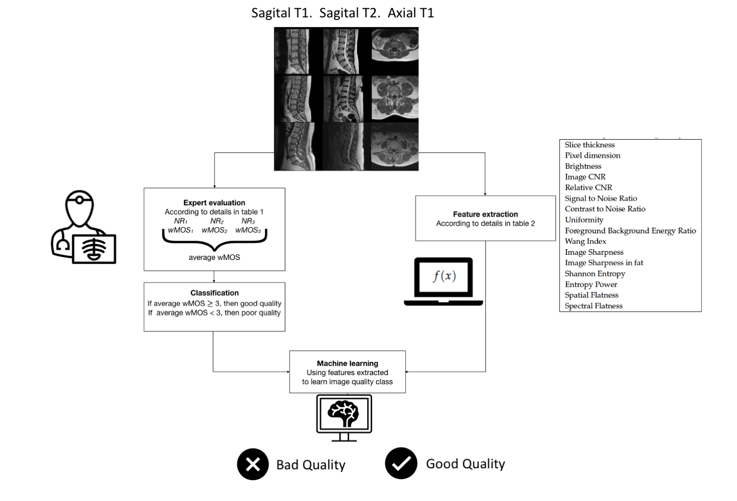
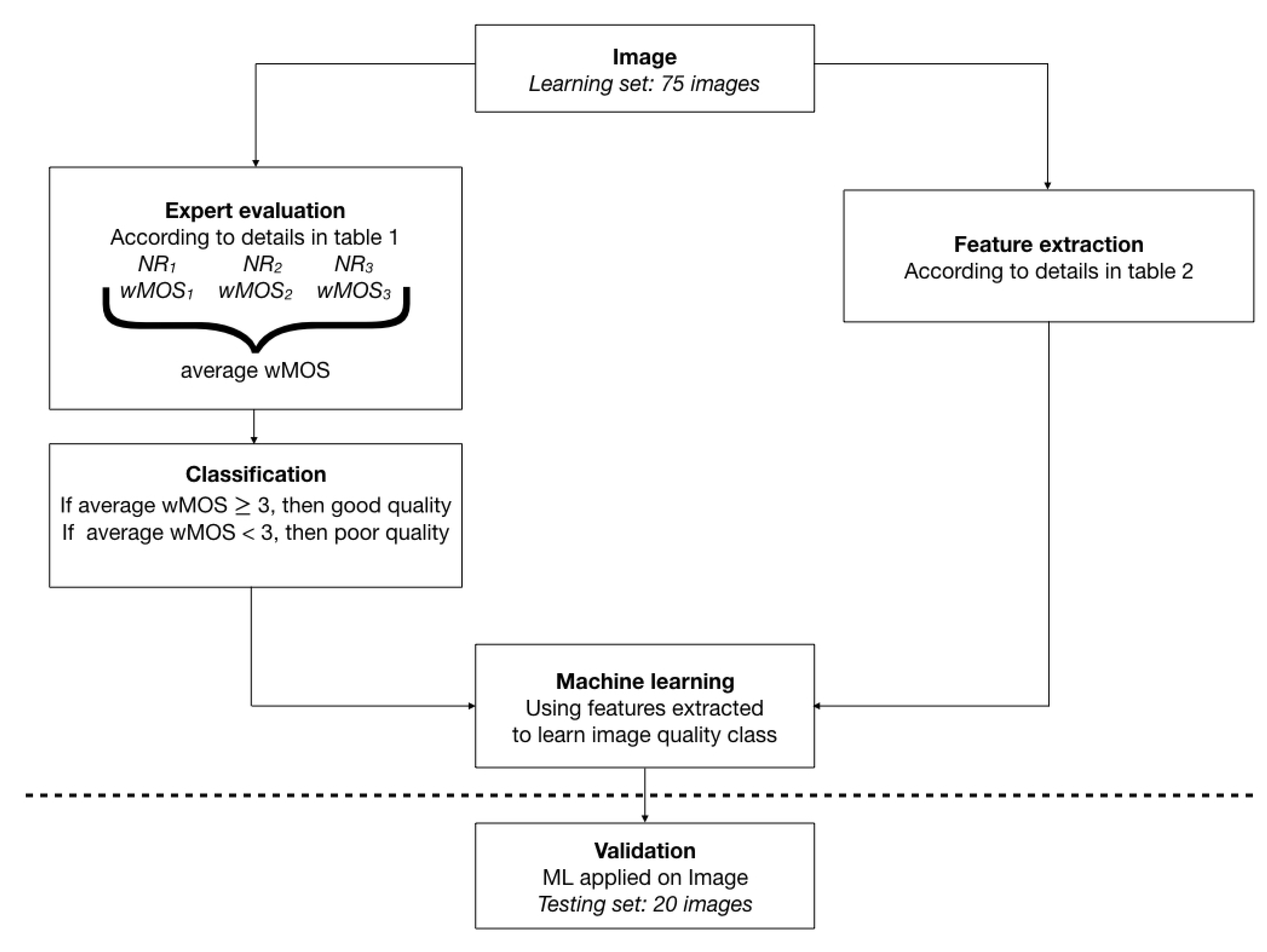
2. Methods and Materials
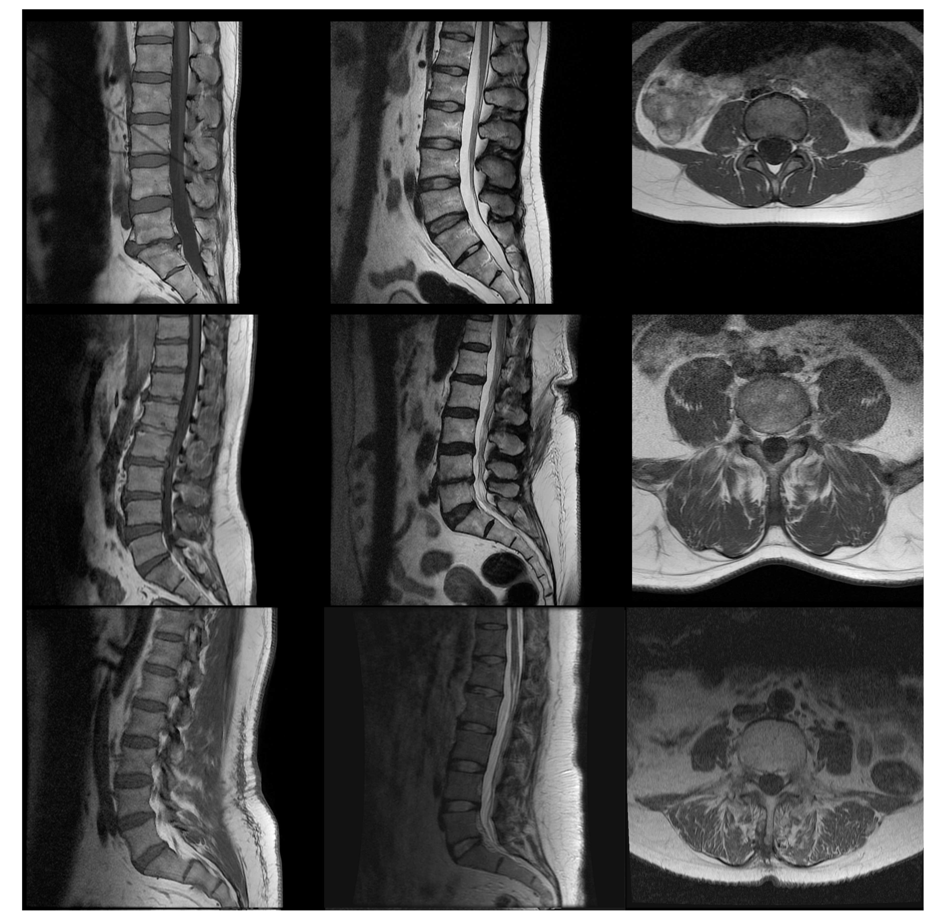
A Global processing pipeline is schematized in Figure 1 and undertaken for each one of the three image types independently. On the one hand, each exam is evaluated separately by three neuro-radiologists in their regular settings for image visualization, each one blind to the evaluation of the other NR, according to a previous list of criteria agreed on and detailed in Section 2.2. According to its average evaluation between the three NR, the exam is classified as “good image quality” if its Mean Opinion Score (MOS) is greater than or equal to 3, corresponding to the qualifiers regular, good or excellent in the subjective evaluation, or as “deficient image quality” otherwise, corresponding to the use of qualifiers bad or poor in the subjective evaluation. On another hand, a list of features is the extracted features from the images, as detailed in Section 2.3. These features are fed to a classifier. Five systems were tested: Linear Discriminant Analysis (LDA), Quadratic Linear Analysis (QDA), Support Vector Machine (SVM), Logistic Regression (LogReg) and Multilayer Perceptron (MLP). We will refer to the evaluation by experts as the “subjective evaluation”, and to the evaluation by machine learning from extracted feature as the “objective evaluation”. Ethical approval by our local Ethics Committee was obtained.

2.1. Data Set

The development of the MR lumbar images data set involved 95 exams from different origins: our local hospital contributed with 41 exams and 12 exams from a public database SpineWeb (We have used images from the dataset 1 available at http://spineweb.digitalimaginggroup.ca/Index.php?n=Main.Datasets. accessed on 31 October 2017). Moreover, 42 exams were generated by modifying other original exams to count on a wider range of image quality variations. The modification includes one or a combination of the following:
  • Noise addition, with a standard deviation ranging from 0.001 to 0.8
  • Contrast manipulation using power transform with gamma values ranging from 0.7 to 1.15
  • Convolution with Gaussian kernel, with the kernel used from 3 × 3 to 6 × 6
All image modifications were developed in Matlab (MathWorks, Natick, MA, USA). Each exam includes 3 types of images: T 1 -weighting in axial and sagittal slices and T 2 -weighting in sagittal slices. Each image type was analyzed separately.

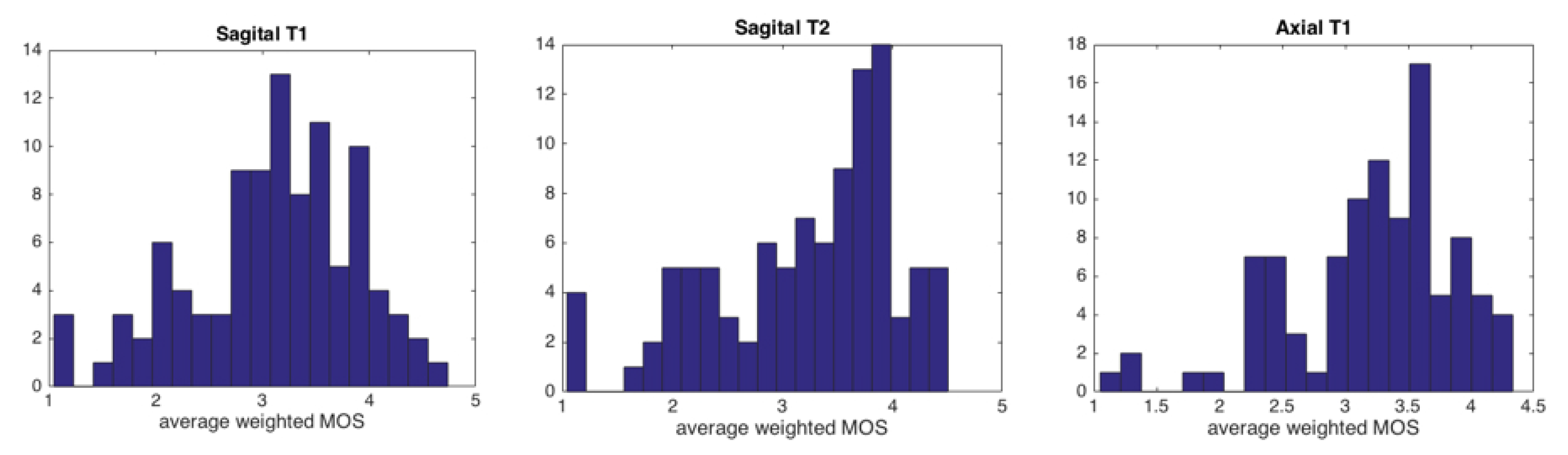
2.2. Subjective Evaluation

Three neuro-radiologists, with from 6 to 26 years of professional experience, participated in this study. First, the DELPHI method was used among these three experts to establish the image evaluation criteria and the relative weightings of these criteria [22,23,24], as shown in Table 1. To obtain such a list, we proceeded as follows: a list of criteria of what was relevant in the image quality was obtained first by an external observation of the radiologists’ method of reviewing each type of image, while they were verbally expressing their observations. This list was then submitted as a questionnaire to the each NR. Agreement on which criterion to use was obtained. Once the list of criteria was defined, agreement was easily obtained by the three NR on their respective weight. Each criterion is evaluated using a Likert scale, with scores corresponding to: 1—bad, 2—poor, 3—regular, 4—good, 5—excellent. According to this scale and the weight of each criterion, each exam obtains one grade per NR, and then a weighted Mean Opinion Score (wMOS) is calculated by averaging the scores given by the three NR.

2.3. Objective Evaluation

Image feature extraction was undertaken in Matlab, in a semi-automatic way. Some features were evaluated on a Region Of Interest (ROI), others over the entire slice. The ROIs were positioned manually within vertebral bodies, intervertebral discs, fatty tissues, psoas, and paravertebral muscle in three different slices located in the center of the acquired volume. Image manipulation was conducted by engineers, blinded to the process and results of the “subjective evaluation”. The dataset is composed of three different cases of MR lumbar images, of T 1 -weighting acquisitions in axial and sagittal orientation and T 2 -weighting in sagittal orientation. Three different slices were obtained for each exam modality. On the one hand, for the sagittal exams ( T 1 and T 2 ), 26 features were extracted from each of the three different slices, obtaining a total of 78 variables. From these features, 12 of them were computed from the whole image and 14 from several ROIs (8 SNR, 2 CNR, 3 Uniformity, and 1 Image Sharpness in fat). Moreover, for the axial exams, 16 features were extracted from each of the three different slices, obtaining 48 variables. From these features, 12 of them were computed from the whole image and four from several ROIs (2 SNR, 1 CNR, and 1 Image Sharpness in fat).
Some features were selected to depict different characteristics known to influence image perception, such as spatial resolution or presence of noise; other features correspond to a mathematical description of the image not directly related to human perception. Some of the features are sensitive to spatial resolution, such as pixel dimension, slice thickness, or quantification of “image sharpness” relative to the presence of borders within the image. Other features are sensitive to the presence of noise or signal homogeneity, such as signal-to-noise ratio (SNR),contrast-to-noise ratio (CNR), or “uniformity” of the signal within an ROI. Some features are sensitive to the presence of artifacts: we used the index proposed by Wang et al. [25], and also quantification of the ratio of the energy present in the signal in the foreground and the background. In the case of aliasing artifacts, the background energy is altered. The Wang index is a no-reference image quality metric made initially to measure distortions caused by JPEG compression on natural images. This measure is explored here for its utility in the noise and intensity non-uniformity detection. It is used in its implementation made public by their authors (https://github.com/dcatteeu/JpegQuality. accessed on 20 July 2019).
Less “intuitive” characteristics were also included so that another approach of image description is taken into account, different from the one trying to quantify parameters that could explain human perception directly, such as contrast or spatial resolution. In this category, we find measures of entropy, spatial, and spectral flatness. Image representations based on histograms are quite popular, and entropy is among the most widely used. Image distortions have been observed to affect the histograms of pixel intensities [26]. The histogram-based Shannon entropy could be an indicator of noise and intensity non-uniformity. An unpredictable image, i.e., nonredundant, in the spatial domain, will tend to have a white or flat looking spectrum. Conversely, predictable images will possess colored spectra; that is, their spectral shapes exhibit peaks. The spectral flatness measure is widely used to quantify signal information and compressibility [27]. A complementary quantity has been proposed, spatial flatness, which quantifies image shape [28].
The features extracted from the images are detailed in Table 2. S represents the pixel intensity, S ¯ i represents the average of intensities in region i. I represents the image and I v a vector created from the image columns. B is the number of intensity levels present in the image, and p k an estimation of the probability of occurrence of the k t h gray level. F represents the Fourier transform of the image and S u v the gradient evaluated in pixel ( u , v ) . N x and N y represent matrix size in x and y direction, respectively, and N p i x stands for the number of pixels present within a specific ROI or foreground or background. The foreground was separated from background first by user interaction, identifying a pixel from each region, then contrast was enhanced by histogram manipulation and equalization, a Wiener filter was applied, and a unique threshold was identified by the Otsu method.

2.4. Machine Learning

In the process for classifying exams into “good” or “deficient” it was decided to apply five techniques of machine learning that are well known and widely used in the state of the art. Linear Discriminant Analysis (LDA) and Quadratic Discriminant Analysis (QDA) are classifiers with a linear or quadratic decision limit, respectively, generated from adjusting the conditional densities of the data classes using the Bayes rule [29]. Another of the most used algorithms is the Support Vector Machine (SVM) technique. The SVM is a supervised learning classifier utilized for the prediction of class labels. It transforms features into a higher dimension space, where it implements the optimal hyperplane that describes the classes. The hyperplane work is based on the maximum margin between itself and those nearest to it. The nearest set of points are called support vectors [30]. Another method is Logistic regression (LogReg), a statistical approach for predicting binary classes. The outcome or target variable is dichotomous in nature, and the model computes the probability of an event occurrence using a logit function [31]. Finally, the Multi layer perceptron (MLP) is a supplement of the feed forward neural network, and consists of three types of layers: the input layer (it receives the input signal to be processed), output layer (It performs the task) and hidden layer (the true computational engine of the MLP). Similar to a feed forward network, in an MLP the data flow in the forward direction from input to output layer and the neurons are trained with the back propagation learning algorithm. MLPs are designed to approximate any continuous function and can solve problems which are not linearly separable. The major use cases of MLP are pattern classification, recognition, prediction and approximation [32]. These five algorithms (LDA, QDA, SVM, LogReg and MLP) were implemented in python 3.6 using the ScikitLearn toolbox in version 0.16.1 [33].
In order to reduce the dimensionality of the input data, the Principal Component Analysis (PCA) technique is applied, which decomposes the data set into a series of orthogonal components that explain a desired amount of variance. In the case of the proposed data set, the amount of features obtained in objective evaluation was reduced applying PCA, the variance was solved by 99%, and 12 principal components were reported. For LDA it is used as a singular value decomposition (SVD) solver which is not based on the calculation of the covariance matrix; instead, it performs a polar decomposition from a square matrix m * n to any other matrix. SVM was implemented using a radio basal kernel (RBF) which is described by ϕ y ( x , l ) = e x p ( y | | x l | | 2 ) ; this causes many dimensions to be created in the dataset and makes it linearly separable. The hyperparameters were selected using a Grid Search Cross Validation.
To avoid overfitting and validate the model, we carried out the simulation study with a 10-fold cross-validation scheme. The averages of the accuracy, precision, recall, F1-score and area under curve (AUC) for testing were estimated for each of the machine learning models. Moreover, the Kappa Index was estimated as the Agreement coefficient.

3. Results

Typical images of “bad” and “good” quality as defined by the experts are shown in Figure 2. The examples aim to emphasize that, even if the difference between a clearly good and a clearly bad image is easy to assess, the subtleties of the in-between range are more difficult to distinguish. Figure 3 presents the distribution of the image quality of our three data sets evaluated by the experts: each of the data sets presents an equilibrated quantity of “good” and “bad” quality images. Axial images are globally better evaluated than sagittal images by all experts.
Agreement between neuro-radiologists about the image quality is rated from fair to substantial in the different types of data sets, as detailed in Table 3. Better agreement in quality image evaluation is found in Sagittal T 2 data sets, with Kappa values of 0.56 ± 0.08 over all cases, while the worst agreement is found in the axial T 1 data set, with Kappa values of 0.38 ± 0.22. NR 1 and NR 2 present the closest agreement in image quality evaluation, even though Kappa values reach only 0.63 ± 0.03, underlining that excellent experts’ agreement is not easy to achieve. Agreement between NR 2 and NR 3 is even lower, only 0.35 ± 0.12.
Figure 4 shows correlation coefficients between MOS and each feature used in the objective quality assessment. Most correlation coefficients calculated in the case of Axial T 1 images are close to 0, showing that no clear linear relation between MOS and each feature separately exists that could by itself identify “good” or “bad” quality images. A very similar trend is observed in the case of Sagittal T 2 images. Considering Sagittal T 1 images, a few correlation coefficients rise to a magnitude of 0.6, uniformity measured in the vertebra or spectral flatness, but this correlation is not strong enough to explain the classification obtained by subjective assessment.
Classification performance metrics obtained for the five ML models are described in Table 4. In general, the SVM showed superior performance in most cases, followed by LDA and MLP. Furthermore, it can be observed that QDA showed the lowest performance. The SVM achieved an accuracy of over 73% in all cases, it reached 77% in Sagittal T 2 as well as a recall of 89% for this same image. On the other hand, the reported AUC reflects a good discriminatory precision by showing values higher than 70%.
The agreement between each neuro-radiologist and the classification by SVM, being the best learning case, was evaluated and is displayed in Table 5. Agreement in all cases was moderate, showing the best results between SVM and NR 1 . The exam type that showed the best agreement between expert, Sagittal T 2 , showed one of the best agreements between SVM and NR, 0.48 ± 0.05. Conversely, Axial T 1 images, which showed the lowest kappa index between NR, are also the ones that present the lowest kappa index between SVM and neuro-radiologist, of 0.37 ± 0.04. In comparison with what is shown in Table 4, results are slightly improved for LDA, but no significant change is seen in SVM (data not shown).

4. Discussion

The agreement that is observed between the three radiologists, in Table 3, vary from fair to substantial. Even though it is usually easy to be in agreement to establish a diagnosis, to reach agreement on subjective quality perception led to more discussions. Two examples can be found in [34,35], where agreement among experts was moderate in subjective determination of glaucomatous visual field profession, and in subjective evaluation of sublingual microcirculation images, respectively. In our understanding, the observed differences in subjective evaluations could reflect the different manners that the neuro-radiologists use in their interactions with the images. Each of them was trained in a different school, some began practicing neurosurgery before neuro-radiology which might reflect different subjective expectation on image quality. The training radiologists receive has been shown to influence their behavior in reading images [36]. Differences in perceptions also could come from their differences in experience, such as [36,37] emphasize. In our understanding, the differences in subjective perceptions seen in this work reflect the reality of the existence of a range of experts evaluations. The system proposed here includes the variety of experts perceptions, in a way that would be more potentially more robust and more generalizable in future works, than one that reflects only the subjective evaluation of one expert, be it the most experienced perception or not.
The experts’ perception of image quality is emulated with good accuracy, 75.3 ± 2.4% on average in the testing condition, using the Support Vector Machine. A wide range of features was extracted either from the entire image or from specific user-defined ROI in relation to lumbar anatomy. Features include characteristics known to influence image perception, such as signal to noise ratio or spatial resolution, but other less “intuitive” parameters were also taken into account such as spectral flatness or entropy. The image quality evaluation obtained from the non-linear combination of these characteristics, shown in Table 4, is in better agreement with the experts’ view than each of the features taken individually, as depicted in Figure 4. Comparing the results obtained with the literature is complex since there is no similar model based on the same set of image type and machine learning technique used. However, it can be mentioned that the performance obtained is lower than reported by Nakanishi et al. [38], who evaluated the efficacy of a fully automated method for assessing the image quality (IQ) of coronary computed tomography angiography (CCTA), obtaining an AUC of 0.96 and a kappa index for the agreement between automated and visual IQ assessment of 0.67. Similarly, the performance obtained is lower than that reported by Küstner et al. [39], who proposed a new machine-learning-based reference-free MR image quality assessment framework, including the concept of active learning and applying classifiers such as SVM and Deep Neural Networks. Although these authors report a high percentage of accuracy (93.7%), they did not perform an evaluation of concordance with experts, making this comparison difficult. However, performance results were closer to reported by Pizarro et al. [40], who applied an SVM algorithm in the quality assessment of structural brain images, using global and region of interest (ROI) automated image quality features developed in-house and obtaining an accuracy of 80%. On the other hand, on natural images, correlation coefficients between subjective vs. predictive MOS have been obtained close to 80% [41]. When using reference images, correlation coefficients published are close to 95% [17] or 96% [42], using sparse representation and kernel ridge regression. Yet their implementation was applied to natural images, with the possibility of estimation of visual information fidelity. It would be interesting to apply these methodologies described in the state of the art to the lumbar MRI data set and compare their performance with the algorithm proposed in this research. However, some conditions prevent its realization. For example, in the case of the algorithm proposed by Küstner et al., it involved a Deep Learning model in its classifiers, which cannot be applied in our work due to the limited database. On the other hand, Nakanishi et al. proposed an automated estimation using specific features of CCTA, and the novelty of this method is largely in obtaining these features prior to the application of the Machine Learning model. Since the characteristics obtained in lumbar MRI are different, the method proposed by Nakanishi to our work does not have much scalability. Finally, Pizarro et al. present a model very similar to the one developed in our research since they use the MRI image, extract its main characteristics and use the SVM as a classifier. Beyond the type of image used, a key step that differs between the two methods is the dimensionality reduction performed with the PCA in our work, so we consider it unnecessary to replicate what was developed by these authors.
It is interesting to note that the results obtained here were obtained through the machine learning of the three experts, taking into account more than an individual point of view. In the case of this application, the agreement between experts was not always qualified as “excellent”, and the machine must learn different points of view. This is a common problem faced in machine learning, and the results obtained here show good performance in general. The human judgment or decision are based in several variables that may seem reasonable, however there exists many unobserved information that cannot be captured. Meanwhile, machine learning methods rely only on the available data obtained from quantifiable features [43,44,45,46].
These results are encouraging with respect to the possibility of developing an automated system that could monitor not only “mathematical image quality” but also image quality perceived by experts, who are the real final users of medical images. The method still needs to be fully automatized to avoid human interaction for the positioning of the Region-Of-Interest in the analysis. These are only preliminary results, as the proposed method was tested on three types of exams so far, and the number of exams, of sites and vendors needs to be increased. This would increase the number of observations of “bad quality” images obtained with no artificial manipulation, and therefore should refine the capacity of the method proposed here to discriminate between image qualities. One of the specificities of the images types that were selected here is that they were acquired with a spine MRI coil, which means that the signal within the images was not homogeneous. Working with these kinds of images does not represent conditions common to all kinds of MR images.
There is a discussion on how to define image quality in medical applications. A crisp definition of good vs. bad quality was used in the present case. The use of a fuzzy definition of transition between types might bring the behavior of this system closer to that of the human experts. It is important to emphasize that this system should be apprehended as a constant monitoring solution and that the interest is not in detecting when one single exam was of poor quality but when, as a whole, the trend of the MR system is deteriorating from an image quality point of view.

5. Conclusions

In conclusion, a method is presented here, where feasibility of the emulation of expert perception of image quality in three types of lumbar MR images is shown. Good accuracy is obtained in the set of images used, Sagittal T 1 , Sagittal T 2 , and Axial T 1 , of 75 ± 2.4% on average in the testing condition, using a Support Vector Machine to construct the classifier. Using a non linear combination of quality features extracted from the images, an emulation is obtained of the combined views of three different experts, whose agreement on image quality varies between fair and substantial. Even though the actual implementation still relies on user interaction to extract certain features from the images, the results are promising with respect to a potential implementation in monitoring image quality online with the image acquisition process.
Future works could include further features, such as block kurtosis of DCT coefficients [47], dominant eigenvalues of the covariance matrix [48] or kernel ridge regression [42] for instance. Other machine learning techniques, closer to deep neural networks [49], might also improve the performance of image assessment. The method in its essence can be applied to other kind of images, while modifying the definition of localization of ROI in agreement with the organs observed. All other features proposed in Table 2 can be extracted for different kinds of medical images.
Further work is needed to confirm the observations in other experimental conditions and to other types of images, using for instance MR images in other anatomical area, or computed tomography images. The automatic assessment of medical image quality is probably an issue that will occur more frequently as many artificial intelligence systems are developed based on large-scale databases, whose quality has been questioned [50]. Moreover, this study could be extended by increasing the number of subjective evaluators and introducing multi-criteria decision-making techniques [51] to support the variability among the users.

Author Contributions

The contributions of each author to the research carried out are listed below: conceptualization, S.C., P.C., R.R., J.V. and R.S.; methodology, S.C., P.C., R.R., J.V., M.Q., C.S., A.V. and R.S.; validation, S.C., P.C., R.R., J.V. and R.S.; formal analysis, S.C., J.S.C., L.M., C.S., A.V. and R.S.; investigation, S.C., J.S.C., C.S. and A.V.; data curation, L.M., Gamaliel Huerta; writing—original draft preparation, S.C., J.S.C., M.Q. and R.S.; writing—review and editing, L.M., P.C., R.R., J.V., C.S., M.Q. and A.V.; funding acquisition, S.C. and R.S. All authors have read and agreed to the published version of the manuscript.

Funding

This publication has received funding from Millennium Science Initiative of the Ministry of Economy, Development and Tourism, grant Nucleus for Cardiovascular Magnetic Resonance.

Institutional Review Board Statement

The study was conducted according to the guidelines of the Declaration of Helsinki, and approved by the Ethics Committee of SERVICIO DE SALUD VALPARAISO SAN ANTONIO (protocol code 50/2016, date of approval 19 October 2016).

Informed Consent Statement

As data was extracted from a previously anonymized database in the hospital, with no possibility for the investigators or other person to access the identity of the individual, with the aim of the study focused on the technical quality of images, the Ethics Committee granted the authorization of waiving patient consent.

Data Availability Statement

The ethical committee did not authorize the release of the data publicly. However, we have used public dataset 1 from the SpineWeb database available at http://spineweb.digitalimaginggroup.ca/Index.php?n=Main.Datasets.

Conflicts of Interest

The authors declare no conflict of interest.

References

  1. Krupinski, E.A.; Jiang, Y. Anniversary paper: Evaluation of medical imaging systems. Med Phys. 2008, 35, 645–659. [Google Scholar] [CrossRef] [Green Version]
  2. Commission, I.E. (Ed.) IEC62464—1 Magnetic Resonance Equipment for Medical Imaging—Determination of Essential Image Quality Parameters; British Standard Institute (BSI): London, UK, 2019. [Google Scholar]
  3. Attard, S.; Castillo, J.; Zarb, F. Establishment of image quality for MRI of the knee joint using a list of anatomical criteria. Radiography 2018, 24, 196–203. [Google Scholar] [CrossRef]
  4. Chow, L.S.; Paramesran, R. Review of medical image quality assessment. Biomed. Signal Process. Control 2016, 27, 145–154. [Google Scholar] [CrossRef]
  5. Kamble, V.; Bhurchandi, K.M. No-reference image quality assessment algorithms: A survey. Optik 2015, 126, 1090–1097. [Google Scholar] [CrossRef]
  6. Xu, S.; Jiang, S.; Min, W. No-reference/Blind Image Quality Assessment: A Survey. IETE Tech. Rev. 2017, 34, 223–245. [Google Scholar] [CrossRef]
  7. Narvekar, N.D.; Karam, L.J. A no-reference perceptual image sharpness metric based on a cumulative probability of blur detection. In Proceedings of the 2009 International Workshop on Quality of Multimedia Experience, IEEE, San Diego, CA, USA, 29–31 July 2009; pp. 87–91. [Google Scholar] [CrossRef]
  8. Varadarajan, S.; Karam, L.J. An improved perception-based no-reference objective image sharpness metric using iterative edge refinement. In Proceedings of the 2008 15th IEEE International Conference on Image Processing, IEEE, San Diego, CA, USA, 12–15 October 2008; pp. 401–404. [Google Scholar] [CrossRef]
  9. Winter, R.M.; Leibfarth, S.; Schmidt, H.; Zwirner, K.; Mönnich, D.; Welz, S.; Schwenzer, N.F.; la Fougère, C.; Nikolaou, K.; Gatidis, S.; et al. Assessment of image quality of a radiotherapy-specific hardware solution for PET/MRI in head and neck cancer patients. Radiother. Oncol. 2018, 128, 485–491. [Google Scholar] [CrossRef] [PubMed] [Green Version]
  10. Alexander, D.C.; Zikic, D.; Ghosh, A.; Tanno, R.; Wottschel, V.; Zhang, J.; Kaden, E.; Dyrby, T.B.; Sotiropoulos, S.N.; Zhang, H.; et al. Image quality transfer and applications in diffusion MRI. NeuroImage 2017, 152, 283–298. [Google Scholar] [CrossRef] [PubMed]
  11. Veloz, A.; Moraga, C.; Weinstein, A.; Hernández-García, L.; Chabert, S.; Salas, R.; Riveros, R.; Bennett, C.; Allende, H. Fuzzy general linear modeling for functional magnetic resonance imaging analysis. IEEE Trans. Fuzzy Syst. 2019, 28, 100–111. [Google Scholar] [CrossRef]
  12. Chabert, S.; Verdu, J.; Huerta, G.; Montalba, C.; Cox, P.; Riveros, R.; Uribe, S.; Salas, R.; Veloz, A. Impact of b-Value Sampling Scheme on Brain IVIM Parameter Estimation in Healthy Subjects. Magn. Reson. Med. Sci. 2019, mp–2019. [Google Scholar] [CrossRef] [PubMed] [Green Version]
  13. Sotelo, J.; Salas, R.; Tejos, C.; Chabert, S.; Uribe, S. Análisis cuantitativo de variables hemodinámicas de la aorta obtenidas de 4D flow. Rev. Chil. Radiol. 2012, 18, 62–67. [Google Scholar] [CrossRef] [Green Version]
  14. Veloz, A.; Orellana, A.; Vielma, J.; Salas, R.; Chabert, S. Brain Tumors: How Can Images and Segmentation Techniques Help; Diagnostic Techniques and Surgical Management of Brain Tumors, IntechOpen: London, UK, 2011; ISBN 978-953-307-589-1. [Google Scholar] [CrossRef] [Green Version]
  15. Saavedra, C.; Salas, R.; Bougrain, L. Wavelet-based semblance methods to enhance the single-trial detection of event-related potentials for a BCI spelling system. Comput. Intell. Neurosci. 2019, 2019. [Google Scholar] [CrossRef] [Green Version]
  16. Gupta, P.; Bampis, C.G.; Glover, J.L.; Paulter, N.G., Jr.; Bovik, A.C. Multivariate Statistical Approach to Image Quality Tasks. J. Imaging 2018, 4, 117. [Google Scholar] [CrossRef] [Green Version]
  17. Liu, L.; Dong, H.; Huang, H.; Bovik, A.C. No-reference image quality assessment in curvelet domain. Signal-Process.-Image Commun. 2014, 29, 494–505. [Google Scholar] [CrossRef]
  18. Alfaro-Almagro, F.; Jenkinson, M.; Bangerter, N.; Andersson, J.; Griffanti, L.; Douaud, G.; Sotiropoulos, S.; Jbabdi, S.; Hernandez-Fernandez, M.; Vallee, E.; et al. Image processing and Quality Control for the first 10,000 brain imaging datasets from UK Biobank. NeuroImage 2018, 166, 400–424. [Google Scholar] [CrossRef]
  19. Rosen, A.F.; Roalf, D.R.; Ruparel, K.; Blake, J.; Seelaus, K.; Villa, L.P.; Ciric, R.; Cook, P.A.; Davatzikos, C.; Elliott, M.A.; et al. Quantitative assessment of structural image quality. NeuroImage 2018, 169, 407–418. [Google Scholar] [CrossRef] [PubMed]
  20. Chacon, G.; Rodriguez, J.; Bermudez, V.; Florez, A.; Del Mar, A.; Pardo, A.; Lameda, C.; Madriz, D.; Bravo, A. A score function as quality measure for cardiac image enhancement techniques assessment. Rev. Latinoam. Hipertens. 2019, 14, 180–186. [Google Scholar]
  21. Barrett, H.H.; Kupinsky, M.A.; Müeller, S.; Halpern, H.; Moris, J., III; Dwyer, R. Objective assessment of image quality VI: Imaging in radiation therapy. Phys. Med. Biol. 2013, 58, 8197–8213. [Google Scholar] [CrossRef] [PubMed] [Green Version]
  22. Linstone, H.A.; Turoff, M. The Delphi Method: Techniques and Applications; Addison-Wesley: Reading, PA, USA, 1975. [Google Scholar]
  23. Boulkedid, R.; Abdoul, H.; Loustau, M.; Sibony, O.; Alberti, C. Using and Reporting the Delphi Method for Selecting Healthcare Quality Indicators: A Systematic Review. PLoS ONE 2011, 6, e20476. [Google Scholar] [CrossRef] [PubMed]
  24. Sá Dos Reis, C.; Gremion, I.; Richli Meystre, N. Consensus about image quality assessment criteria of breast implants mammography using Delphi method with radiographers and radiologists. Insights Imaging 2020, 11, 56. [Google Scholar] [CrossRef] [Green Version]
  25. Zhou, W.; Sheikh, H.R.; Bovik, A.C. No-reference perceptual quality assessment of JPEG compressed images. In Proceedings of the IEEE International Conference on Image Processing, Rochester, NY, USA, 22–25 September 2002; Volume 1, p. I. [Google Scholar] [CrossRef] [Green Version]
  26. Hadjidemetriou, E.; Grossberg, M.; Nayar, S. Multiresolution histograms and their use for recognition. IEEE Trans. Pattern. Anal. Mach. Intell. 2004, 26, 831–847. [Google Scholar] [CrossRef] [PubMed]
  27. Jayant, N.; Noll, P. Digital Coding of Waveforms: Principles and Applications to Speech and Video; Prenctice Hall: Hoboken, NJ, USA, 1984. [Google Scholar]
  28. Woodward, J.; Carley-Spencer, M. No-reference image quality metrics for structural MRI. Neuroinformatics 2006, 4, 243–262. [Google Scholar] [CrossRef]
  29. Bowles, M. Machine Learning in Python: Essential Techniques for Predictive Analysis; John Wiley & Sons: Hoboken, NJ, USA, 2015. [Google Scholar]
  30. Khan, M.A.; Sharif, M.; Javed, M.Y.; Akram, T.; Yasmin, M.; Saba, T. License number plate recognition system using entropy-based features selection approach with SVM. IET Image Process. 2017, 12, 200–209. [Google Scholar] [CrossRef]
  31. Denoeux, T. Logistic regression, neural networks and Dempster–Shafer theory: A new perspective. Knowl.-Based Syst. 2019, 176, 54–67. [Google Scholar] [CrossRef] [Green Version]
  32. Golovko, V. Deep learning: An overview and main paradigms. Opt. Mem. Neural Netw. 2017, 26, 1–17. [Google Scholar] [CrossRef]
  33. Pedregosa, F.; Varoquaux, G.; Gramfort, A.; Michel, V.; Thirion, B.; Grisel, O.; Blondel, M.; Prettenhofer, P.; Weiss, R.; Dubourg, V.; et al. Scikit-learn: Machine Learning in Python. J. Mach. Learn. Res. 2011, 12, 2825–2830. [Google Scholar]
  34. Tanna, A.; Bandi, J.; Budenz, D.; Feuer, W.J.; Feldman, R.; Herndon, L.; Rhee, D.; Whiteside-de Vos, J. Interobserver agreement and intraobserver reproducibility of the subjective determination of glaucomatous visual field progression. Ophthalmology 2011, 118, 60–65. [Google Scholar] [CrossRef] [PubMed]
  35. Lima, A.; López, A.; van Genderen, M.E.; Hurtado, F.J.; Angulo, M.; Grignola, J.C.; Shono, A.; van Bommel, J. Interrater Reliability and Diagnostic Performance of Subjective Evaluation of Sublingual Microcirculation Images by Physicians and Nurses: A Multicenter Observational Study. Shock 2015, 44, 239–244. [Google Scholar] [CrossRef] [PubMed]
  36. Ganesan, A.; Alakhras, M.; Brennan, P.; Mello-Thoms, C. A review of factors influencing radiologists’ visual search behaviour. J. Med. Imaging Radiat. Oncol. 2018, 62, 747–757. [Google Scholar] [CrossRef] [PubMed]
  37. Kammerer, S.; Schulke, C.; Leclaire, M.; Schwindt, W.; Velasco Gonzalez, A.; Zoubi, T.; Heindel, W.; Buerke, B. Impact of Working Experience on Image Perception and Image Evaluation Approaches in Stroke Imaging: Results of an Eye-Tracking Study. Rofo 2019, 191, 836–844. [Google Scholar] [CrossRef] [PubMed] [Green Version]
  38. Nakanishi, R.; Sankaran, S.; Grady, L.; Malpeso, J.; Yousfi, R.; Osawa, K.; Ceponiene, I.; Nazarat, N.; Rahmani, S.; Kissel, K.; et al. Automated estimation of image quality for coronary computed tomographic angiography using machine learning. Eur. Radiol. 2018, 28, 4018–4026. [Google Scholar] [CrossRef]
  39. Küstner, T.; Gatidis, S.; Liebgott, A.; Schwartz, M.; Mauch, L.; Martirosian, P.; Schmidt, H.; Schwenzer, N.F.; Nikolaou, K.; Bamberg, F.; et al. A machine-learning framework for automatic reference-free quality assessment in MRI. Magn. Reson. Imaging 2018, 53, 134–147. [Google Scholar] [CrossRef] [Green Version]
  40. Pizarro, R.A.; Cheng, X.; Barnett, A.; Lemaitre, H.; Verchinski, B.A.; Goldman, A.L.; Xiao, E.; Luo, Q.; Berman, K.F.; Callicott, J.H.; et al. Automated quality assessment of structural magnetic resonance brain images based on a supervised machine learning algorithm. Front. Neuroinform. 2016, 10, 52. [Google Scholar] [CrossRef] [PubMed] [Green Version]
  41. Saad, M.A.; Bovik, A.C.; Charrier, C. A DCT Statistics-Based Blind Image Quality Index. IEEE Signal Process. Lett. 2010, 17, 583–586. [Google Scholar] [CrossRef] [Green Version]
  42. Yuan, Y.; Guo, Q.; Lu, X. Image quality assessment: A sparse learning way. Neurocomputing 2015, 159, 227–241. [Google Scholar] [CrossRef]
  43. Kleinberg, J.; Lakkaraju, H.; Ludwig, J.; Mullainathan, S. Human decisions and machine predictions. Q. J. Econ. 2018, 133, 237–293. [Google Scholar] [PubMed]
  44. Chabert, S.; Mardones, T.; Riveros, R.; Godoy, M.; Veloz, A.; Salas, R.; Cox, P. Applying machine learning and image feature extraction techniques to the problem of cerebral aneurysm rupture. Res. Ideas Outcomes 2017, 3, e11731. [Google Scholar] [CrossRef] [Green Version]
  45. Veloz, A.; Chabert, S.; Salas, R.; Orellana, A.; Vielma, J. Fuzzy spatial growing for glioblastoma multiforme segmentation on brain magnetic resonance imaging. In Iberoamerican Congress on Pattern Recognition; Springer: Berlin/Heidelberg, Germany, 2007; pp. 861–870. [Google Scholar]
  46. Castro, J.S.; Chabert, S.; Saavedra, C.; Salas, R. Convolutional neural networks for detection intracranial hemorrhage in CT images. In Proceedings of the 5th Congress on Robotics and Neuroscience, CRoNe 2019, Valparaíso, Chile, 27–29 February 2020; pp. 37–43. [Google Scholar]
  47. Caviedes, J.; Gurbuz, S. No-reference sharpness metric based on local edge kurtosis. In Proceedings of the IEEE International Conference on Image Processing, Rochester, NY, USA, 22–25 September 2002; Volume 3, pp. 53–56. [Google Scholar]
  48. Wee, C.; Paramesran, R. Image sharpness measure using eigenvalues. In Proceedings of the 2008 9th International Conference on Signal Processing, Beijing, China, 26–29 October 2008; Volume 9, pp. 840–843. [Google Scholar]
  49. Jayageetha, J.; Vasanthanayaki, C. Medical Image Quality Assessment Using CSO Based Deep Neural Network. J. Med. Syst. 2018, 42, 224. [Google Scholar] [CrossRef] [PubMed]
  50. Oakden-Rayner, L. Exploring Large-scale Public Medical Image Datasets. Acad. Radiol. 2019. in Press. [Google Scholar] [CrossRef] [PubMed] [Green Version]
  51. Torres, R.; Salas, R.; Astudillo, H. Time-based hesitant fuzzy information aggregation approach for decision making problems. Int. J. Intell. Syst. 2018, 29, 579–595. [Google Scholar] [CrossRef]
Figure 1. Representation of the workflow used for each image type: T 1 -weighted sagittal and axial and T 2 -weighted sagittal. Details in text.
Applsci 11 06616 g001
Figure 2. Examples of images from (left column) sagittal T 1 , (center column) sagittal T 2 , (right column) axial T 1 , with (first row) high quality according to the experts (weighted Mean Opinion Scores (wMOS) between 4.3 and 4.7), (second row) average quality (wMOS between 3.1 and 3.2) and (third row) low quality (wMOS between 2.7 and 2.8). The examples shown here were not manipulated by us to modify their quality.
Applsci 11 06616 g002
Figure 3. Average weighted Mean Opinion Scores (wMOS) histogram distributions in our three data types, obtained from the experts’ evaluation. From left to right: sagittal T 1 -, sagittal T 2 - and axial T 1 -weighted images.
Applsci 11 06616 g003
Figure 4. Correlation coefficients calculated between wMOS and each of the different features extracted, applied to the three image types.
Applsci 11 06616 g004
Table 1. List of criteria used for the subjective image quality evaluation, elaborated by three neuro-radiologists, using the DELPHI method. Weighted Mean Opinion Score (wMOS) was calculated using the weights listed in the second column of this table. A higher criterion weight implies a greater importance for this specific criterion.
Exam TypeCriterion WeightCriterion
Sagittal T 1 2/50Visualization of vertebral bodies
2/50Visualization of spinal cone
3/50Visualization of facet joints
2/50Signal from bone marrow
5/50Overall evaluation
Sagittal T 2 3/50Signal homogeneity in vertebral bodies
1/50Visualization of the entrance of basivertebral
venous plexuses
3/50Contrast between vertebral body and
intervertebral disc
3/50Spinal cone visualization
3/50Homogeneity of spinal cord signal
5/50Distinction between spinal roots
5/50Overall evaluation
Axial T 1 1/50Similarity of signal between muscles:
paravertebral and psoas
5/50Definition of the edge of the intervertebral
discs
1/50Visualization of fascias or grooves of
subcutaneous fat
1/50Root path through epidural fat
5/50Overall evaluation
Table 2. List of features extracted for the objective image quality evaluation. Variables are explained in the main text.
FeatureDefinitionApply to
Slice thicknessFrom DICOM metadataWhole image
Pixel dimensionFrom DICOM metadataWhole image
BrightnessAverage intensityWhole image
Image CNR m a x ( I ) m i n ( I ) Whole image
Relative CNR I m a g e C N R B r i g h t n e s s Whole image
Signal to Noise Ratio S N R i S ¯ i σ 0.655 1 In sagittal exams: applied on
three different ROIs in vertebral bodies,
in fatty tissues and two intervertebral
discs. In axial exams: applied on
ROI in psoas and paravertebral
muscles and one in fatty tissues.
Contrast to Noise Ratio C N R i j ( S ¯ i S ¯ j ) σ 0.655 1 In sagittal exams: applied
on vertebral bodies vs. disc,
and vertebral body and disc vs. fat.
In axial exams: applied on fatty tissues
vs. psoas and paravertebral muscles.
Uniformity U i U i = 1 A A D i S i ¯ where
A A D i = h = 1 N p i x S h S ¯ i N p i x
In sagittal exams: applied on ROIs in three
vertebral bodies
Foreground Background Energy Ratio FBER E f E b where E = u = 1 N p i x S u 2 within
foreground and background resp.
Whole image
Wang IndexSee [25] for detailsWhole image
Image Sharpness 1 N x N y u = 1 N x v = 1 N y S u v S u v 2 S u v Whole image
Image Sharpness in fatSame as Image Sharpness, but applied in ROI within fatROI within fat
Shannon Entropy k = 1 B p k l o g ( p k ) Whole image
Entropy Power S p e c t r a l F l a t n e s s * u = 1 N x v = 1 N y S u v I ¯ 2 N x N y Whole image
Spatial Flatness Π k = 1 N x N y I v ( k ) 2 1 N x N y 1 N x N y k = 1 N x N y I v ( k ) 2 Whole image
Spectral Flatness Π k = 1 N x N y F v ( k ) 2 1 N x N y 1 N x N y k = 1 N x N y F v ( k ) 2 Whole image
Table 3. Kappa index of agreement between neuro-radiologists (NR). The column on the right and the bottom line indicate mean ± standard deviation. We considered as “substantial” agreement kappa indices between 0.61 and 0.8, as “moderate” agreement values between 0.41 and 0.60 and as “fair” agreement values between 0.21 and 0.40.
NR 1 vs. NR 2 NR 1 vs. NR 3 NR 2 vs. NR 3
Sagittal T 1 0.660.390.340.46 ± 0.17
Sagittal T 2 0.600.620.470.56 ± 0.08
Axial T 1 0.630.290.230.38 ± 0.22
0.63 ± 0.030.43 ± 0.170.35 ± 0.12
Table 4. Metrics of classifier models with respect to subjective Mean Opinion Score (MOS) attributed by experts.
MetricImageLDAQDALogRegSVMMLP
Sagittal T 1 0.7400.7130.7210.7630.731
AccuracySagittal T 2 0.7130.6320.6890.7720.649
Axial T 1 0.7670.6340.7470.7260.726
Sagittal T 1 0.7310.4670.5180.6730.635
PrecisionSagittal T 2 0.7690.6860.7170.7370.686
Axial T 1 0.7170.5370.7000.6220.670
Sagittal T 1 0.6250.2750.5830.8170.692
RecallSagittal T 2 0.6750.5150.6000.8900.605
Axial T 1 0.7750.6420.7250.7500.675
Sagittal T 1 0.6310.3400.5350.7190.646
F1 scoreSagittal T 2 0.7050.5530.6400.7970.735
Axial T 1 0.7250.5780.6930.6740.648
Sagittal T 1 0.7270.7770.7460.7920.801
AUC ROCSagittal T 2 0.7100.7160.7630.7590.735
Axial T 1 0.7910.7400.7800.7470.792
Table 5. Kappa index of agreement between SVM results and each neuro-radiologist (NR).
SVM vs. NR 1 SVM vs. NR 2 SVM vs. NR 3
Sagittal T 1 0.530.370.560.49 ± 0.10
Sagittal T 2 0.520.490.420.48 ± 0.05
Axial T 1 0.380.410.330.37 ± 0.04
0.48 ± 0.080.42 ± 0.060.44 ± 0.12
Publisher’s Note: MDPI stays neutral with regard to jurisdictional claims in published maps and institutional affiliations.

