Multi-Class Classification of Lung Diseases Using CNN Models

Abstract

In this study, we propose a multi-class classification method by learning lung disease images with Convolutional Neural Network (CNN). As the image data for learning, the U.S. National Institutes of Health (NIH) dataset divided into Normal, Pneumonia, and Pneumothorax and the Cheonan Soonchunhyang University Hospital dataset including Tuberculosis were used. To improve performance, preprocessing was performed with Center Crop while maintaining the aspect ratio of 1:1. As a Noisy Student of EfficientNet B7, fine-tuning learning was performed using the weights learned from ImageNet, and the features of each layer were maximally utilized using the Multi GAP structure. As a result of the experiment, Benchmarks measured with the NIH dataset showed the highest performance among the tested models with an accuracy of 85.32%, and the four-class predictions measured with data from Soonchunhyang University Hospital in Cheonan had an average accuracy of 96.1%, an average sensitivity of 92.2%, an average specificity of 97.4%, and an average inference time of 0.2 s.

1. Introduction

In the field of image processing in deep learning [1,2], Convolutional Neural Network (CNN) [3], which is a key technology used primarily, has received tremendous attention. Following the great success of AlexNet [4], performance improvement models such as VGG [5], ResNet [6], and InceptionNet [7] have continued to evolve, and new studies are still being made to occupy State-of-the-Art (SOTA) [8].

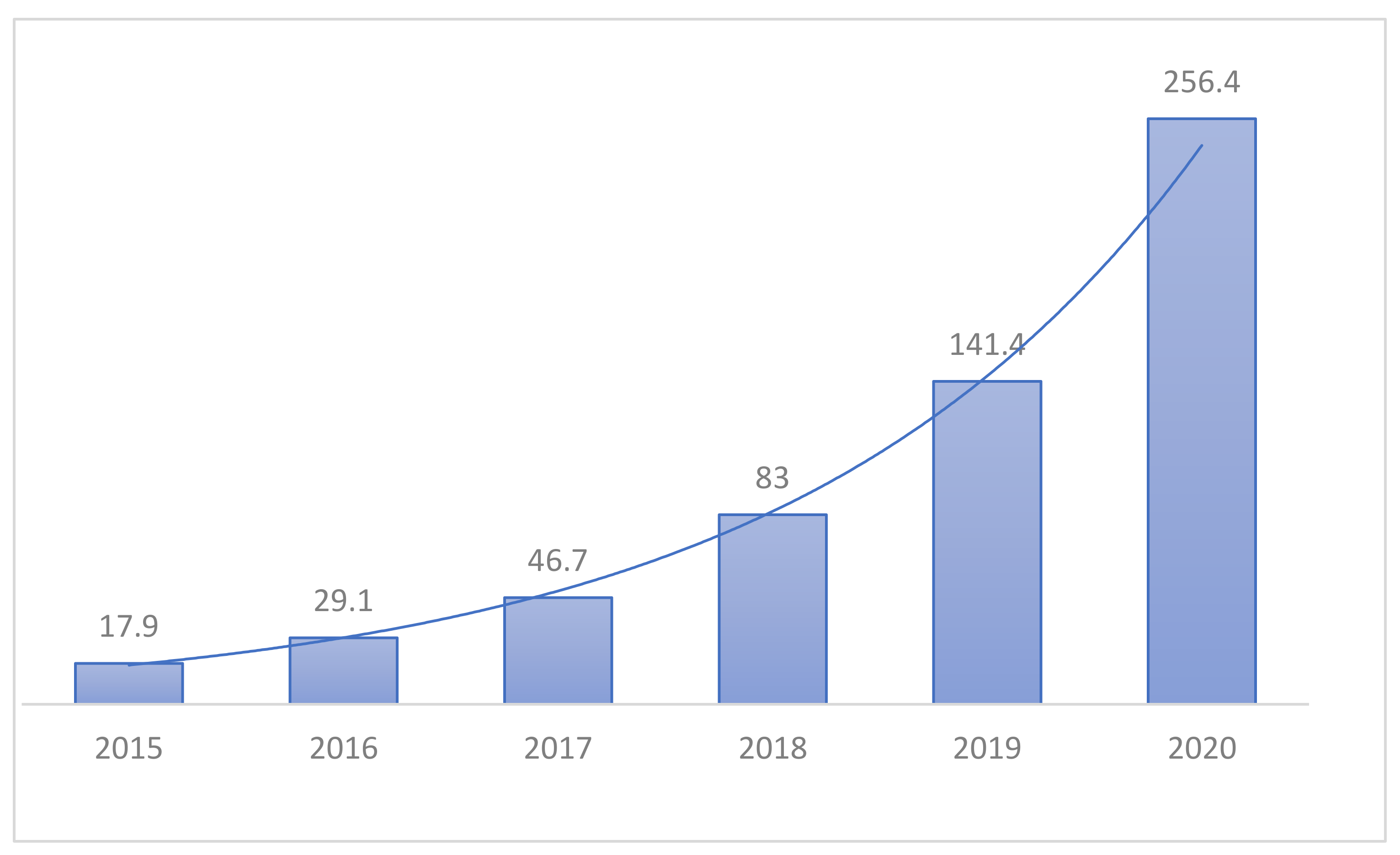
Unlike previous machine learning methods, which required a lot of user intervention, Hyundai Deep Learning is seeking convergence in many areas due to its end-to-end input and output capabilities and ease of access. The medical field is also paying attention to deep learning as a role to assist medical staff in diagnosing in line with this trend. In Korea, various AI startup companies such as Beuno, Rooney, and JLK Inspection are established, and working with medical institutions on projects for various diseases, as shown in Figure 1. With the rise of COVID-19, studies on lung diseases are also underway, especially on Pneumonia. However, research on other lung diseases is relatively lacking in Korea, especially Tuberculosis [9,10,11].

Therefore, in this paper, we propose a multi-class classification model that can cover a wider range of lung diseases by learning a total of four classes, from three lung diseases such as Pneumonia, Pneumothorax, and Tuberculosis, to Normal which is the negative state.

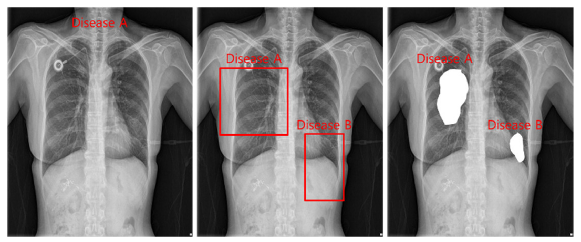
The tasks of deep learning currently utilized in health care are divided into classification, detection, and segmentation, as shown in Figure 2. Models used in all tasks utilize heavy and accurate SOTA models due to the nature of the medical field requiring refinement.

Classification is a task that divides negatives and positives by learning images and labels of diseases and is a method that focuses on learning for inferring disease names. For detection, a Bounding Box is marked around the location of a disease, and the disease name and Bounding Box coordinates are learned to infer the location information of the disease. Segmentation is a method of inferring the disease pixel by pixel by learning the location pixel of the disease.

On the other hand, medical images include continuous images such as Computerized Tomography (CT) and various postures such as posteroanterior chest view (PA), erect anteroposterior chest view (AP), Lateral, and Decubitus, so it is necessary to clarify the shape for learning. Therefore, the following assumptions are made. First, the captured image is a cross-sectional CR X-ray image. Second, the image is taken only in the PA and AP positions. Third, information on the location of the disease is not provided. As such, this study assumes that the medical staff infers the disease name by using the PA and AP images as input images in the model.

2. Lung Diseases

2.1. Pneumonia

Pneumonia disease is an infection that provokes lungs’ air sacs [12]. The air sacs load with fluid or pus causing symptoms such as cough, fever, chills, and trouble breathing. Symptoms of Pneumonia can vary from mild to severe and may include cough, fever, shortness of breath, shallow breathing, stabbing chest pain, loss of appetite, low energy, fatigue, nausea, vomiting, and confusion especially in older people.

2.2. Pneumothorax

Pneumothorax disease can be a complete lung collapse or only a part of the lung [13]. While doing heavy activities such as flying, mountain climbing, or scuba diving may cause accidents, lung disease or illness, and changes in air pressure have all been known to potentially cause lung collapse. A minor pneumothorax may increase on its own, but for more serious cases a needle aspiration or chest tube can be inserted to allow the lung to expand. Symptoms of Pneumothorax commonly begin with chest pain, then other problems include stabbing chest pain, shortness of breath, bluish skin, fatigue, rapid breathing, a dry and hacking cough.

2.3. Tuberculosis

Tuberculosis disease is an airborne bacterial infection in lung caused by the organism Mycobacterium tuberculosis that primarily affects the lungs, although other organs and tissues may be involved [14]. Symptoms of Tuberculosis includes a cough that lasts more than 3 weeks, loss of appetite and unintentional weight loss, fever, chills, and night sweats.

3. Related Work

Gabruseva et al. [15] proposed an automatic pneumonia detection using deep learning. The model was based on RetinaNet to output one of the classes “No Lung Opacity/Not Normal”, “Normal”, and “Lung Opacity”. The best validation mean average precision (mAP) is 0.250230. Ibrahim et al. [16] proposed a deep learning method to classify pneumonia from chest X-ray images. The model was based on AlexNet to output multiclass pneumonia. The test accuracy, sensitivity, and specificity of non-COVID-19 viral pneumonia and healthy are 94.05%, 98.19%, and 95.78%, respectively. The test accuracy, sensitivity, and specificity of Bacterial pneumonia and healthy are 91.96%, 91.94%, and 100.00%, respectively. The test accuracy, sensitivity, and specificity of COVID-19 and healthy are 99.16%, 97.44%, and 100.00%, respectively. The test accuracy, sensitivity, and specificity of COVID-19 and non-COVID-19 viral pneumonia are 99.62%, 90.63%, and 99.89%, respectively. The test accuracy, sensitivity, and specificity of COVID-19, bacterial pneumonia, and healthy are 95.00%, 91.30%, and 84.78%, respectively. The test accuracy, sensitivity, and specificity of COVID-19, non-COVID-19 viral pneumonia, bacterial pneumonia, and healthy are 93.42%, 89.18%, and 98.92%, respectively. Loddo et al. [17] proposed COVID-19 diagnosis from CT images using deep learning. Ten models were compared and VGG19 achieved the best accuracy of 98.87%.

4. Data

4.1. Preprocessing

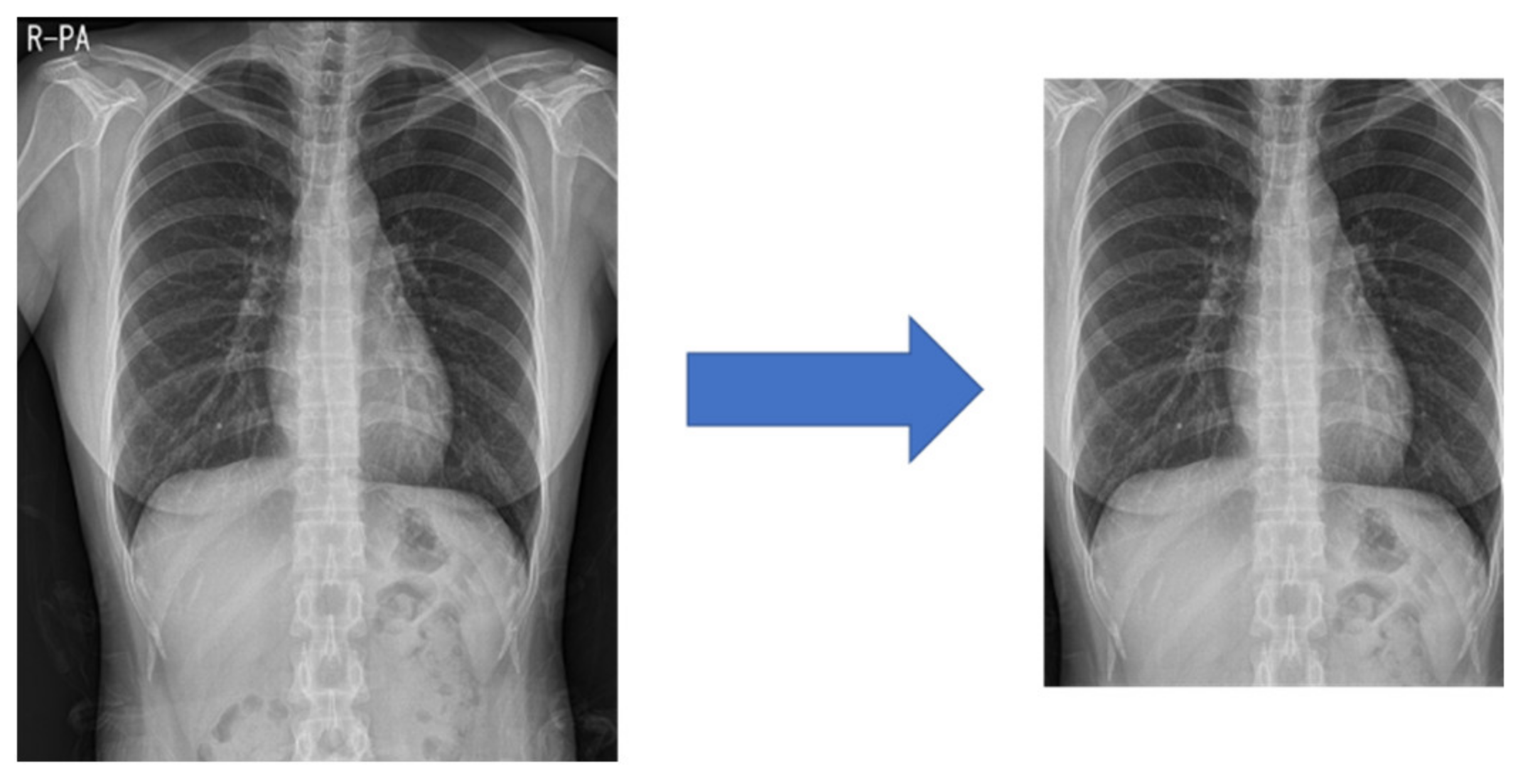
Medical images often have different heights and widths. Most deep learning research ignores this and resizes it, but in this case, the original aspect ratio of the image may be different. Therefore, in this study, to improve the learning performance, the height and width are compared, and the difference in length is cut out from the height or width. After creating a 1:1 ratio, the center pixel is cut out to a size of 87.5%, as shown in Figure 3. This preprocessed image reduces the search range of the CNN to make it easier to learn.

4.2. NIH Dataset

The U.S. National Institutes of Health (NIH) Open Dataset comprises 10,000 PNG images of Normal, Pneumonia, and Pneumothorax [18]. The training data and validation data are divided by 8:2, as shown in

Table 1. NIH dataset.

	Training Data	Validation Data
Normal	2676	669
Pneumonia	1114	278
Pneumothorax	4210	1053
Total	8000	2000

.

4.3. SCH Dataset

The study was approved by the Institutional Review Board of Soonchunhyang University Hospital (2020-12-036-002). We use 51,866 TIF image files provided after de-identification by Soonchunhyang University Hospital. The image is composed of a total of four classes, from Normal, Pneumonia, Pneumothorax to Tuberculosis, and the label information is classified by folder name. Validation data used to know the learning progress is used by collecting and using 500 sheets at the end of each type of training data, as shown in

Table 2. SCH training dataset.

	Training Data	Validation Data
Normal	15,017	500
Pneumonia	14,340	500
Pneumothorax	6730	500
Tuberculosis	9779	500
Total	45,866	2000

. The test data is composed of 4000 unidentified image files given separately for the test, as shown in

Table 3. SCH test dataset.

	Test Data
Normal	1000
Pneumonia	1000
Pneumothorax	1000
Tuberculosis	1000
Total	4000

.

5. Modeling

5.1. Backbone

The encoder model uses EfficientNet [19] B7, which occupies a lot of image classification SOTA. EfficientNet is a model that achieves SOTA by a method called Compound Scaling, and is based on DW (Depthwise Convolution), which divides features by channel and calculates them.

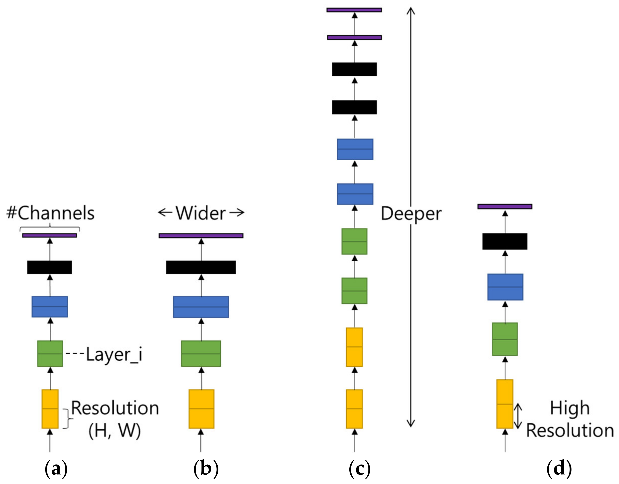
Compound Scaling refers to finding the optimal efficiency by adjusting the model width, model depth, and input image resolution in the basic model as shown in Figure 4. As shown in

Table 4. Performance according to scale change in the same amount of computation.

Model	FLOPS	Top-1 Acc
Baseline model (EfficientNet-B0)	0.4B	77.3%
Scale model by depth (d = 4)	1.8B	79.0%
Scale model by width (w = 2)	1.8B	78.9%
Scale model by resolution (r = 2)	1.9B	79.1%
Compound Scale (d = 1.4,w = 1.2,r = 1.3)	1.8B	81.1%

, the optimized value shows the best performance in terms of computational amount and accuracy.

Backbones of EfficientNet supported by the deep learning framework are models that find and apply the optimal value of Compound Scaling, and are divided into B0, B1, B2, B3, B4, B5, B6, B7, B8, and L2. As the model number increases, the amount of computation doubles.

5.2. Multi GAP

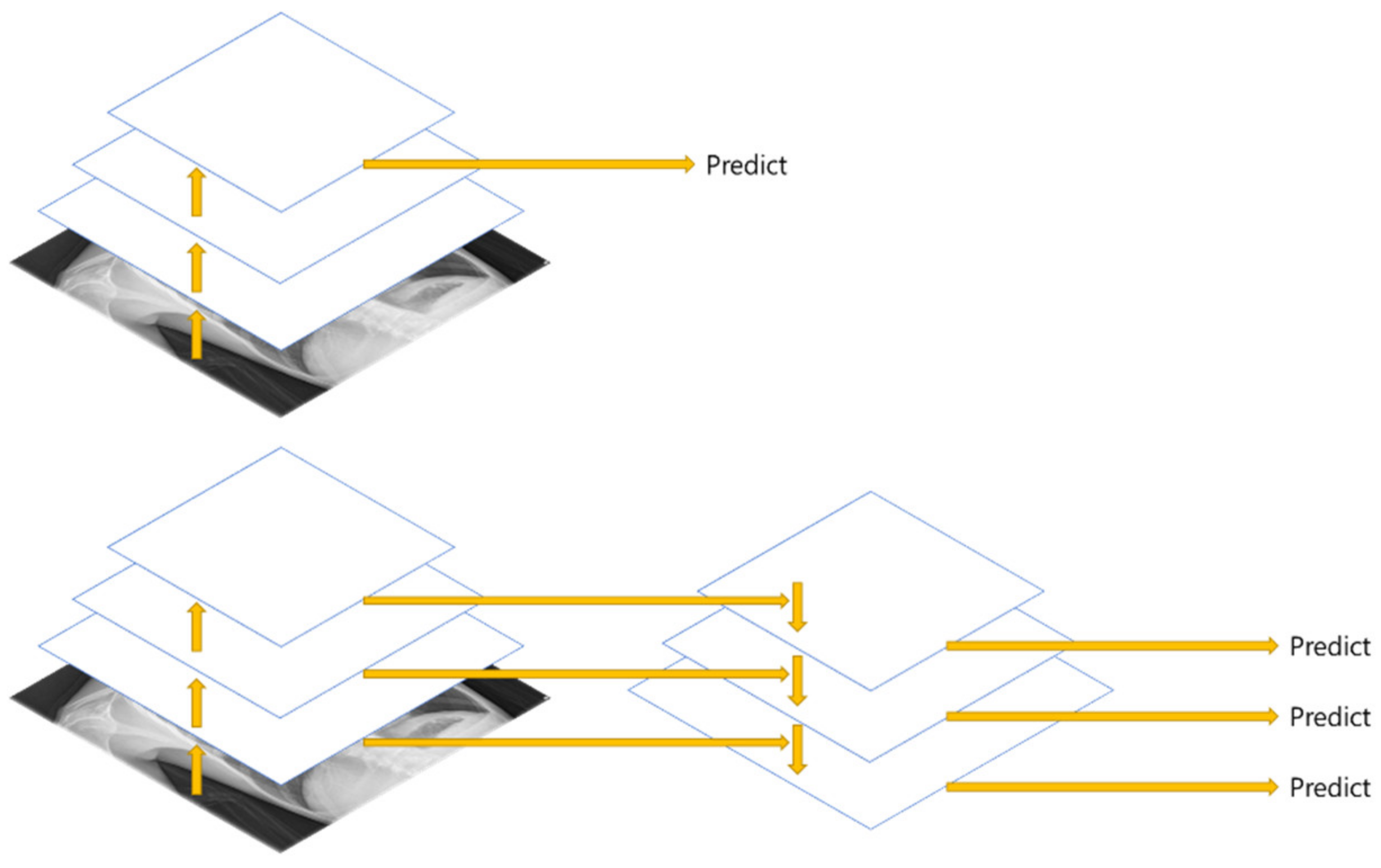
FPN (Feature Pyramid Network) [20] is a structure that extracts multi-scale features, and as shown in Figure 5, more features can be used than the Single Feature Map structure. In this paper, Multi GAP (Global Average Pooling) structure imitating FPN is used.

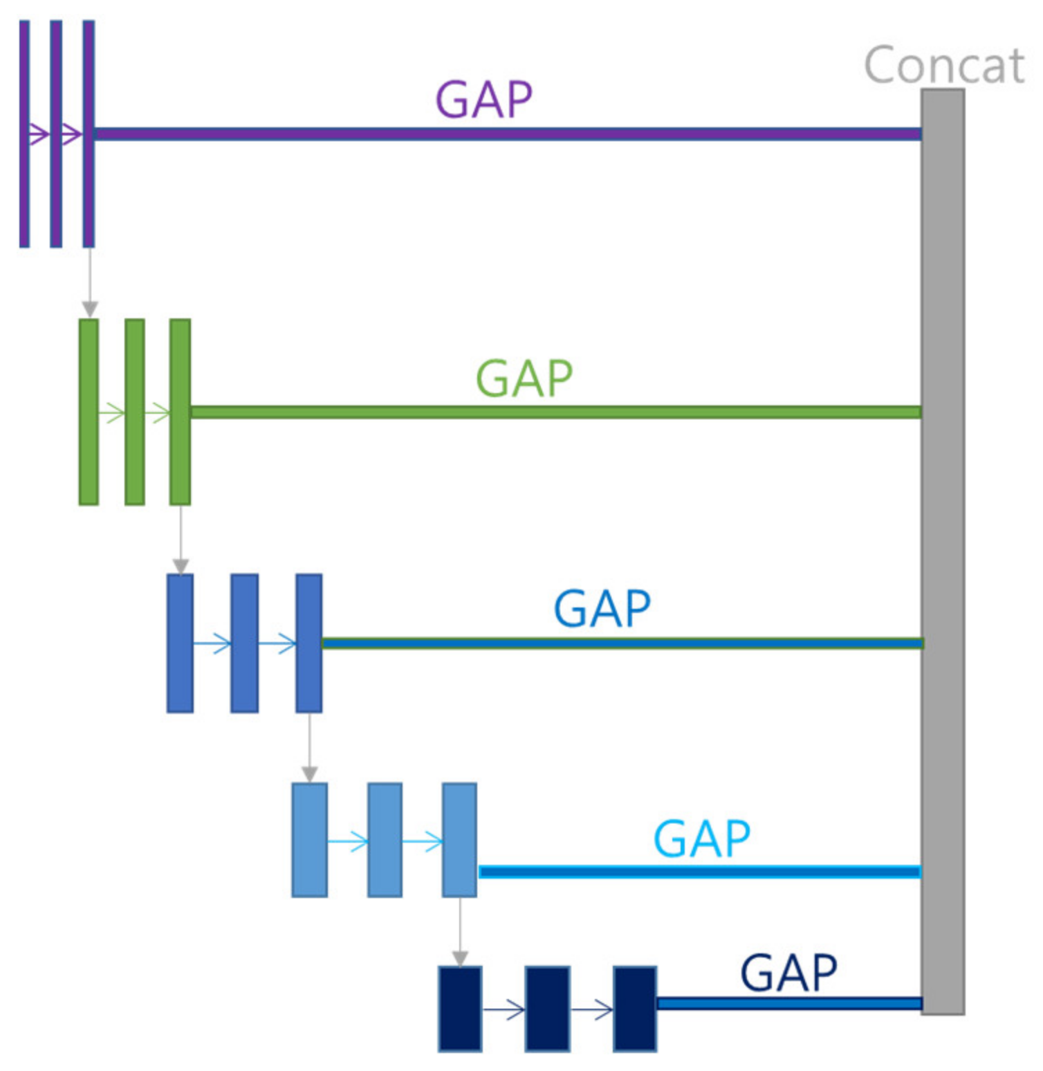
Multi GAP structure refers to a multi structure that extracts features for each layer, compresses them with GAP, and then concatenates them as shown in Figure 6. This structure has the advantage of using many features of FPN, and it is possible to reduce the risk of overload and reduce the amount of computation by compressing each feature with GAP instead of directly converting each feature into FC structure.

5.3. Decoder

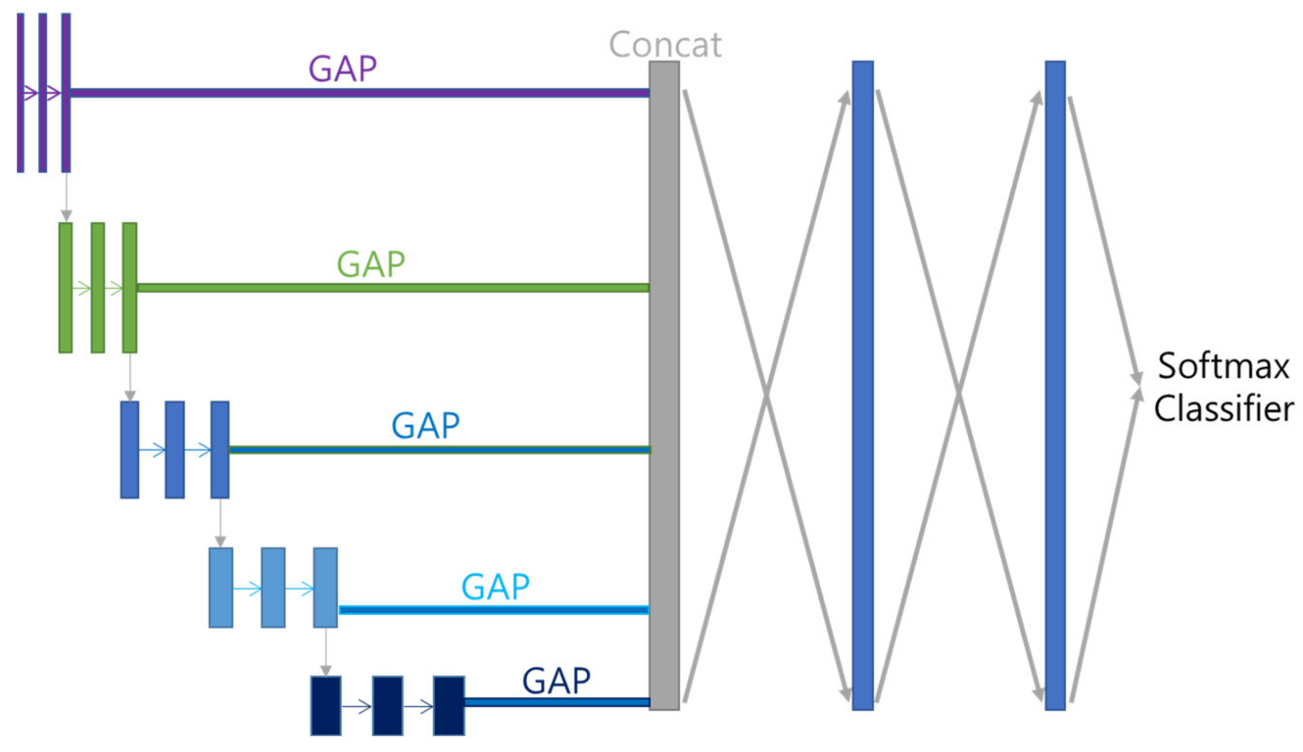
Features acquired with Multi GAP and merged with Concatenate Layer are subjected to 512 FC (Fully Connected Layer) twice, and then multi-class classified using Softmax function. Each class is divided by disease name (including Normal). The overall model structure that combines Encoder and Decoder is shown in Figure 7.

5.4. Regularizations

Since the size of the backbone, EfficienetNet B7, is quite large, the risk of overfitting is also high. To solve this problem, we apply L2 regularization to vectors passing through FC.

$$ǁ\omega ǁ=\sqrt{\left({\omega }_0^2+{\omega }_1^2+\dots +{\omega }_n^2\right)},$$

(1)

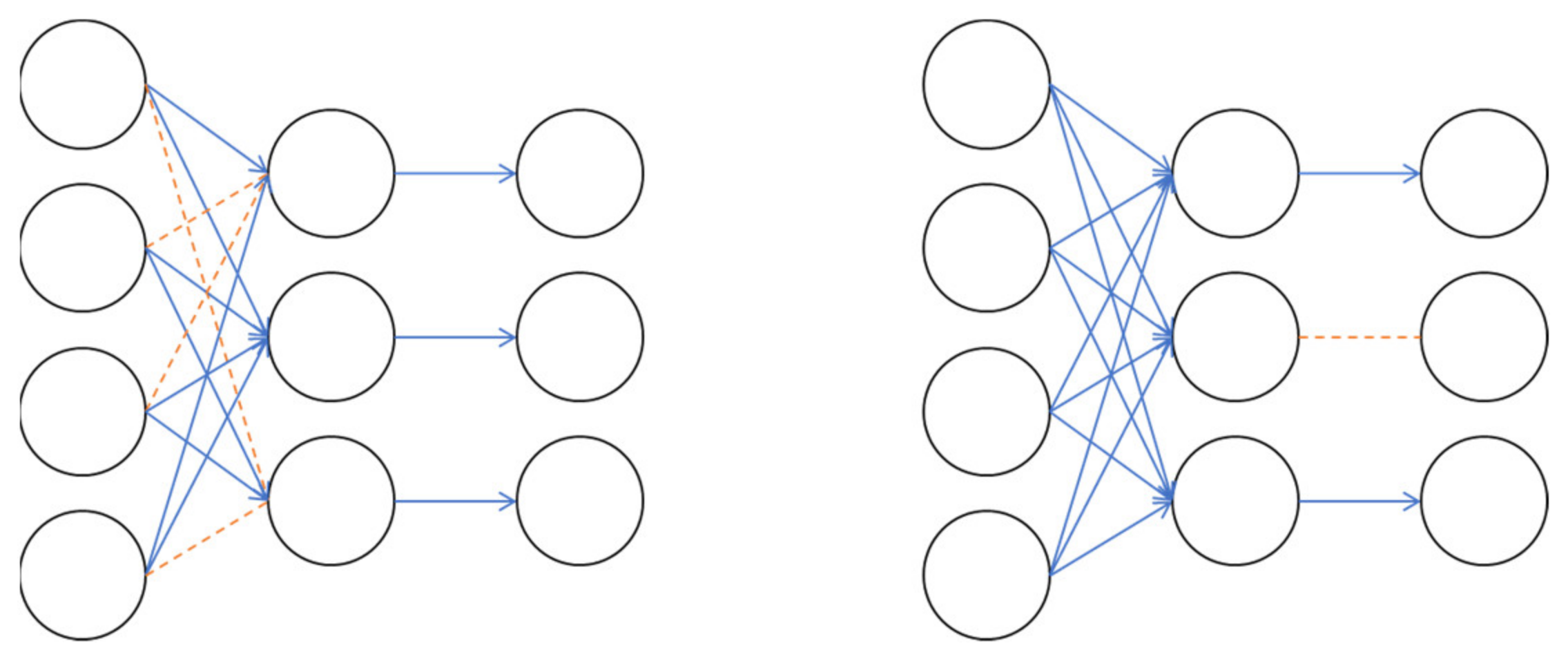
L2 normalization is a method of adding to the loss by multiplying the L2 Norm, which has computed the root of the sum of squares of weights by a certain number, as shown in Equation (1). Also, as shown in Figure 8, Drop Connect, which omits the weight in front of the neuron at a certain rate, and Drop Out, which omits the neuron itself at a certain rate, are used.

6. Benchmarks

Before learning the Cheonan Soonchunhyang Hospital data image, benchmarks are measured with the NIH dataset to compare the preprocessing and model performance. There are a total of 6 compared models including the proposed model, and the encoder structure maintains the basic model in the paper and connects the BottleNeck with GAP. In order to know the influence of the 1:1 ratio Center Crop preprocessing and Multi GAP method of the proposed model, the decoder structure after the FC Layer is set the same.

7. Experiment

7.1. Test Bed

The environment used for the experiment is as follows. The operating system is Linux Ubuntu 18.04 LTS, and we used a desktop PC with Intel CPU i9-9940X 3.30 GHz, 64 G RAM, NVidia Geforce RTX 3090 (1755 MHz, 10,496 cores, 24 GB). All the code was implemented with the deep learning framework Tensorflow 2.5 on CUDA 11 and cuDNN 8, Python 3.9.4.

7.2. Estimate Class Weights

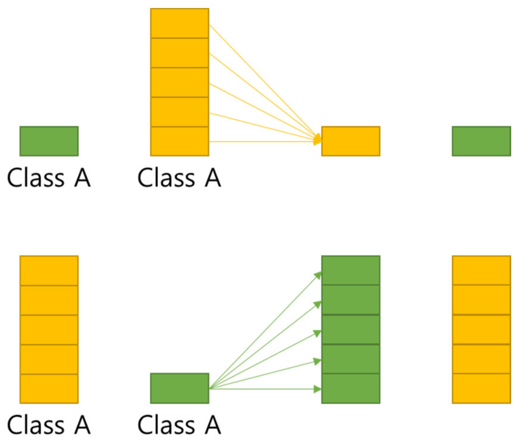
In deep learning, the problem of data imbalance can cause learning that is overly biased to a specific class. As a way to solve this problem, there are the undersampling method that reduces and samples the samples of the class with a large proportion as shown in Figure 9, and the oversampling method that duplicates the samples of the class with a small proportion.

In this study, in order to solve the problem of imbalance between learning data by disease type, a method of varying the update weight for each class was used instead of the sampling method. By assigning a low weight to a disease type with a lot of data and a high weight to a disease type with a small number of diseases, the bias of updates to a specific type of disease was alleviated, as shown in

Table 5. NIH data set weights by disease type.

	Training Data	Class Weight
Normal	2676	0.9965
Pneumonia	1114	2.3937
Pneumothorax	4210	0.6334

and

Table 6. SCH data set weights by disease type.

	Training Data	Class Weight
Normal	15,017	0.7636
Pneumonia	14,340	0.7996
Pneumothorax	6730	1.7038
Tuberculosis	9779	1.1726

.

7.3. Data Augmentations

To prevent overfitting and improve performance, Rand Augment [21] was used for data augmentation. Rand Augment is an augmentation that applies up to N random augments with a maximum random intensity of M.

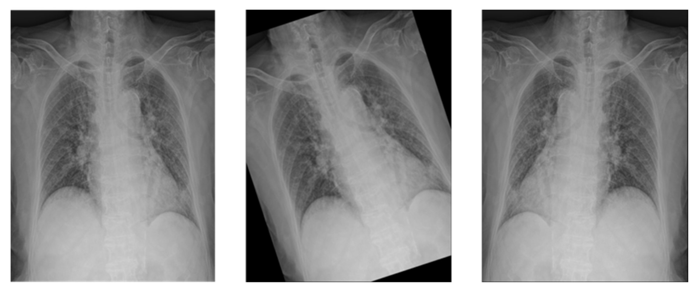
In this study, Augments such as FlipLR, Identity, AutoContrast, Equalize, Rotate, Solarize, Color, Posterize, Contrast, Brightness, Sharpness, ShearX, ShearY, TranslateX, TranslateY were applied. The maximum number N is 2, and the maximum intensity M is set to 28, as shown in Figure 10.

Since deep learning approach is a data-driven approach, the more training data we have, the higher performance we would achieve. Therefore, we did the augmentation in order to increase the number of training sets. By applying Rand augmentation, number of augmented data was randomly created up to maximum 2.

7.4. Fine Tuning

In current deep learning, research [22] has proven that the results of transfer learning or fine tuning with pre-learned weights are superior in performance and stability, and the learning speed is also faster than scratch learning that is learned from scratch. Following this study result, this study also used the weights of “ImageNet” [23] trained as “Noisy Student” [24]. Since the pretrained weights are based on color images in RGB format, the channels of the 1-channel grayscale image were tripled to have 3 channels. Since there was not a lot of data, we did not use the method to freeze the layer. Since the pretrained weights are based on the image size (600, 600), the training data were also image-processed with the same size.

7.5. Scaling

The data scaling method used the standardization method following the method of pretrained weights.

$$ǁz_iǁ=\frac{x_i-\overline{x}}{s} \left(0\le x_i\le 1\right) ,$$

(2)

The standardization formula is as Equation (2). First, the pixel value is divided by 255 (8 bits) or 65,535 (16 bits) to make a decimal number between 0 and 1, and then the overall mean, variance, and standard deviation of the training data set are calculated based on the value. Then subtract the pixel mean from all pixel values made into decimals, and finally divide by the pixel standard deviation.

7.6. Optimizer

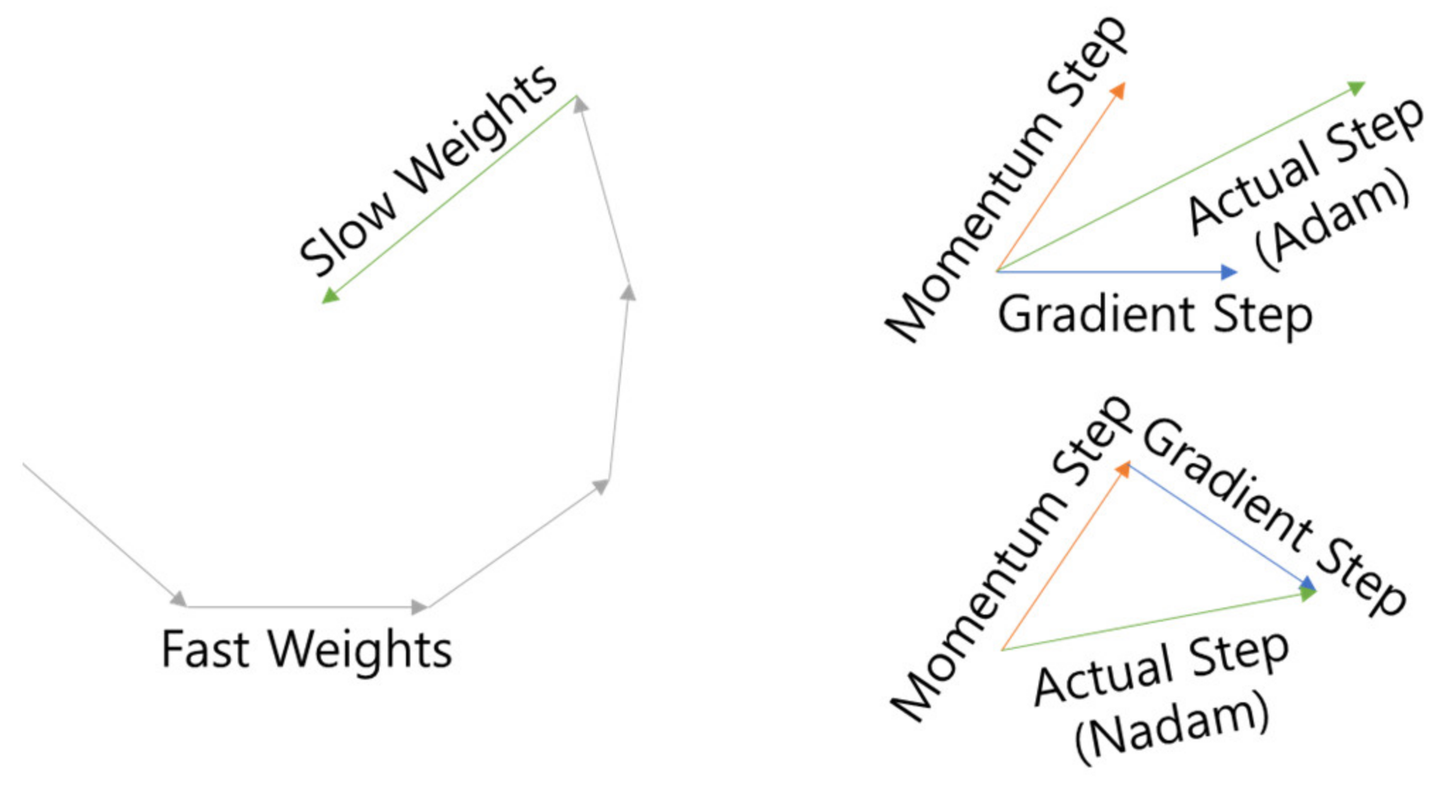
The optimizer used Lookahead [25] as the wrapper and Nadam [26] as the inner optimizer (LA-Nadam). Lookahead is an optimizer that attempts to escape from Local Minima by updating k times (fast weight) and then updating it in the opposite direction (slow weight) once as shown in Figure 11, and Nadam is an optimizer that attempts to escape from Adam [27]’s Momentum as shown in Figure 11 by Nesterov Momentum [28], which is the optimizer. The learning rate is 0.0001, which is 1/10 of Adam’s standard learning rate of 0.001, is used to account for fine-tuning.

$$\begin{gathered} if ǁGradientǁ\ge threshold then \\ Gradient=\frac{threshold}{ǁGradientǁ}\times Gradient \\ end if, \end{gathered}$$

(3)

For the stability of early learning, the Clip Norm value was set to 1. The equation of Clip Norm is the same as (3), and when the L2 Norm value of the Gradient exceeds the Threshold, the Threshold ÷ L2 Norm value is multiplied by the Gradient.

7.7. Learning Rate Scheduling

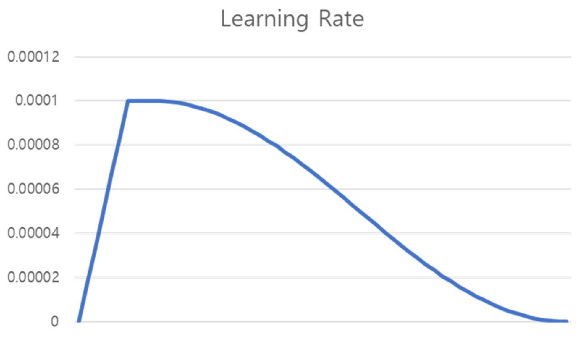
Learning was conducted for a total of 60 epochs. As shown in Figure 12, Warm Up [29] was performed in which the learning rate was linearly increased from 0 to the initial learning rate until 6 epochs, which is 10% of the total epoch, and then proceeded to the initial learning rate until 4 epochs (Flat). For the remaining epochs, the learning rate was gradually decreased using the cosine annealing learning rate [30].

$${\eta }_t=\frac{1}{2} \left(1+\cos \left(\frac{t\pi }{T}\right)\right)\eta ,$$

(4)

Equation of cosine annealing is the same as (4), where η is the learning rate, t is the learning epoch, and T is the total epoch. The learning rate curve applied to warm up, flat, and cosine is shown in Figure 12.

7.8. Label Smoothing

Sigmoid or Softmax, which are used as classifiers in deep learning, approaches 0 and 1, but does not reach them. In general, the GT (Ground Truth) value is set to 0 and 1 and the update proceeds. This setting value makes the model endlessly pursue a value that cannot be reached, so the update of a well-predicted class is also performed constantly. In order to solve this phenomenon, label smoothing [31] is called label smoothing, which relaxes the value of GT so that the model concentrates on the class with poor prediction rather than on the class with good prediction.

$$y_{k^{LS}}=y_k \left(1+\alpha \right)+\alpha /K ,$$

(5)

The label smoothing formula is as in Equation (4), where $y_k$ means GT value, α means the label smoothing ratio, and $K$ means the number of classes. In this study, learning was carried out by setting the label smoothing ratio to 0.1, as shown in

Table 7. Value of GT before and after applying Label Smoothing (NIH).

	Non LS	LS
Negative	0	0.033
Positive	1	0.933

and

Table 8. Value of GT before and after applying Label Smoothing (SCH).

	Non LS	LS
Negative	0	0.025
Positive	1	0.925

.

7.9. Mixed Precision

Common deep learning frameworks proceed with Float32 operation during training. Although Float16 occupies less memory, there was a drawback of somewhat lower accuracy. Mixed Precision [32] solves this problem and mixes the lightness of Float16 operation with the sophistication of Float 32 operation. Mixed Precision uses Float16 for the overall operation and Float32 for the head part that determines the value. And it is a method of calculating all updates with Float32.

In the process of mixing Float16 and Float32, there may be a loss of numbers that exceed the range of Float16 as shown in Figure 10, and this is solved through scaling. When a loss due to a range difference is detected, the corresponding value is scaled to prevent the loss.

By using Mixed Precision, the batch size can be nearly doubled, so the learning speed is very fast, and the performance is similar to or higher than when using Float32. According to Mixed Precision’s paper, as shown in

Table 9. ILSVRC12 Classification Top-1 Accuracy.

Model	Float32	Mixed Precision
AlexNet	56.77%	56.93%
VGG-D	65.40%	65.43%
GoogLeNet(Inception V1)	68.33%	65.43%
Inception V2	70.03%	70.02%
Inception V3	73.85%	74.13%
Resnet 50	75.92%	76.04%

, the results of Mixed Precision were similar or better than Float32. In this study, using Mixed Precision, the existing batch size of 4 was expanded to double that of 8.

7.10. Loss and the Others

Loss used categorical cross-entropy, and Step was set as ‘data set size ÷ batch size’.

Table 10. Hyper Parameters.

Hyper Parameters	Value
Image Resolution	(600, 600)
Number of channels	3
Scaling	Standardization
Optimizer	LA-Nadam
Learning Rate	0.0001
Scheduler	Flat Cosine Anneling with Warm Up
Loss	Categorical Cross-entropy
Label Smoothing	0.1
Augmentations	Rand Augment(2, 28)
Regularizations	Drop Connect 0.4, Drop Out 0.5, L2 Norm 0.01
Max Epoch	60
Batch	8
Classifier	Softmax
Global Policy	Mixed Precision

shows the overall Hyper Parameters.

7.11. Metrics

There are three metrics used for learning evaluation: Accuracy, Sensitivity, and Specificity. In the NIH dataset, the performance of each model is compared with Accuracy, and in the Cheonan Soonchunhyang University data set, all three metrics are measured to measure the precise performance of the proposed model.

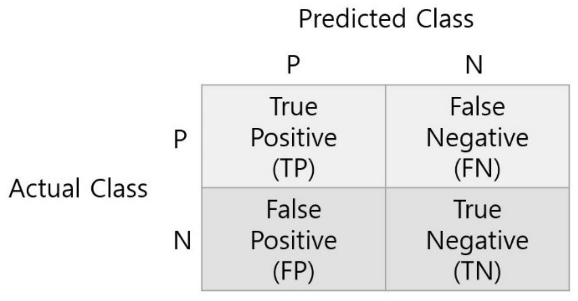
To calculate metrics, first obtain a confusion matrix. Confusion Matrix compares the correct answer with the predicted value as shown in Figure 13, and divides the correct result into TP (True Positive) and TN (True Negative) and the wrong result into FP (False Positive) and FN (False Negative).

$$Accuracy=\frac{TP+TN}{TP+TN+FP+FN} ,$$

(6)

$$Sensitivity=\frac{TP}{TP+TN},$$

(7)

$$Specificity=\frac{TN}{TN+FP},$$

(8)

The formulas for each metric calculated based on the Confusion Matrix are as Equations (6)–(8). Accuracy is a metric that evaluates overall performance, Sensitivity is a metric for whether the model correctly predicted the positive among actual positive samples, and Specificity is a metric to evaluate whether the model correctly predicted the negative among actual negative samples.

8. Results

8.1. NIH Dataset

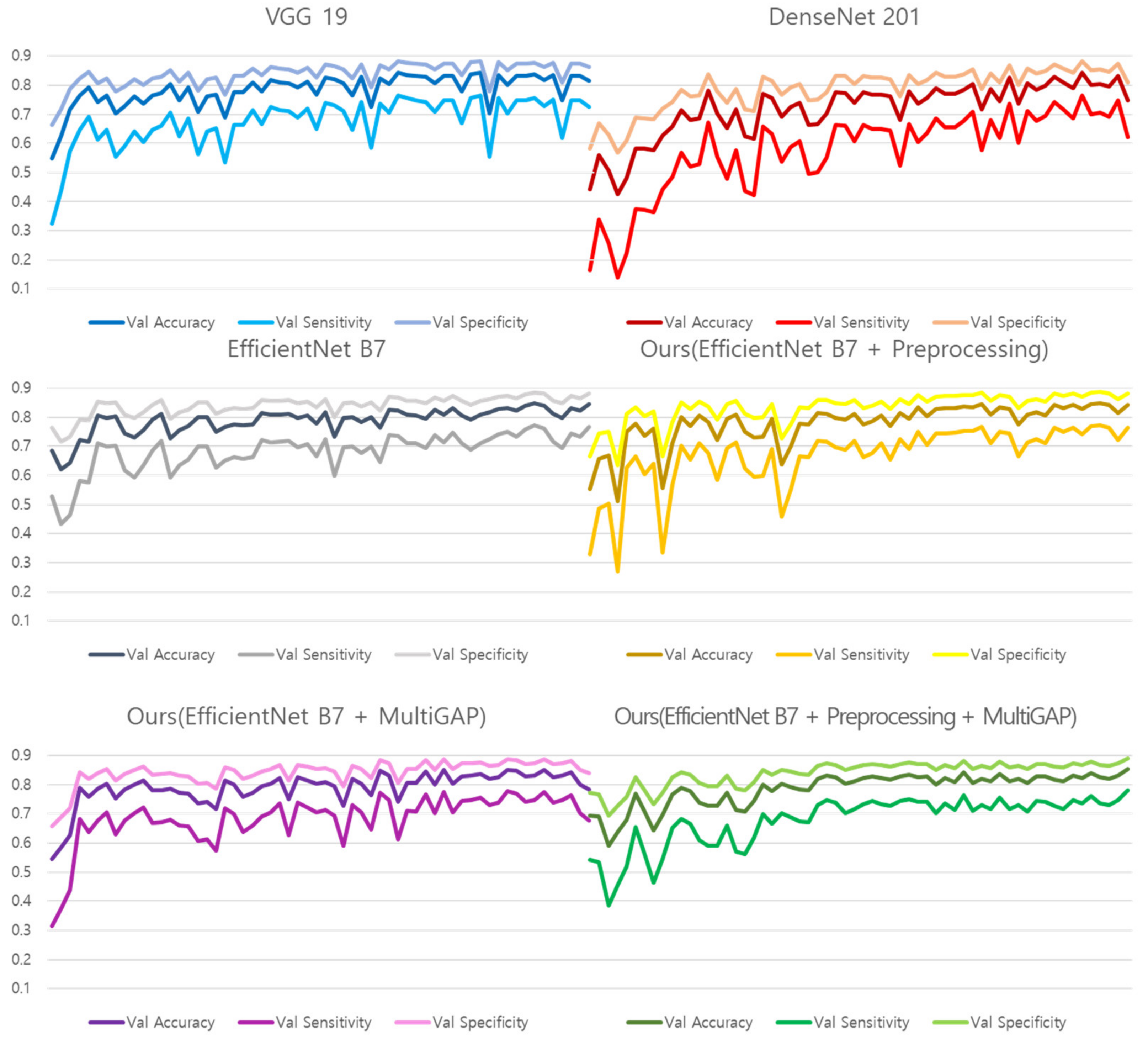
Figure 14 shows the training graphs of models that predicted Normal, Pneumonia, and Pneumothorax by learning 10,000 NIH images. Since validation was used as a test set, the performance was measured based on the learning graph without a separate test process, and the accuracy of a total of 6 models was compared.

Table 11. Validation performance.

Model	Accuracy	Sensitivity	Specificity
VGG 19	84.25%	76.36%	88.18%
DenseNet 201	84.37%	76.56%	88.28%
Vanilla EfficientNet B7	84.76%	77.14%	88.57%
Ours (EfficientNet B7 + Preprocessing)	84.86%	77.29%	88.64%
Ours (EfficientNet B7 + Multi GAP)	85.15%	77.73%	88.86%
Ours (EfficientNet B7 + Preprocessing + Multi GAP)	85.32%	77.97%	88.98%

shows the validation performance of the models created based on the training epoch that recorded the highest number within a total of 60 epochs. Because of the use of Pre-trained weight, it can be converged within 60 epochs. Since the NIH data was not divided like the test dataset, we evaluated the NIH dataset on validation performance only. It can be seen that the proposed model outperforms the comparative models. In particular, the improvement of Accuracy in comparison with Vanilla EfficientNet B7 shows that the proposed preprocessing method and Multi GAP have an effect on performance.

8.2. SCH Dataset

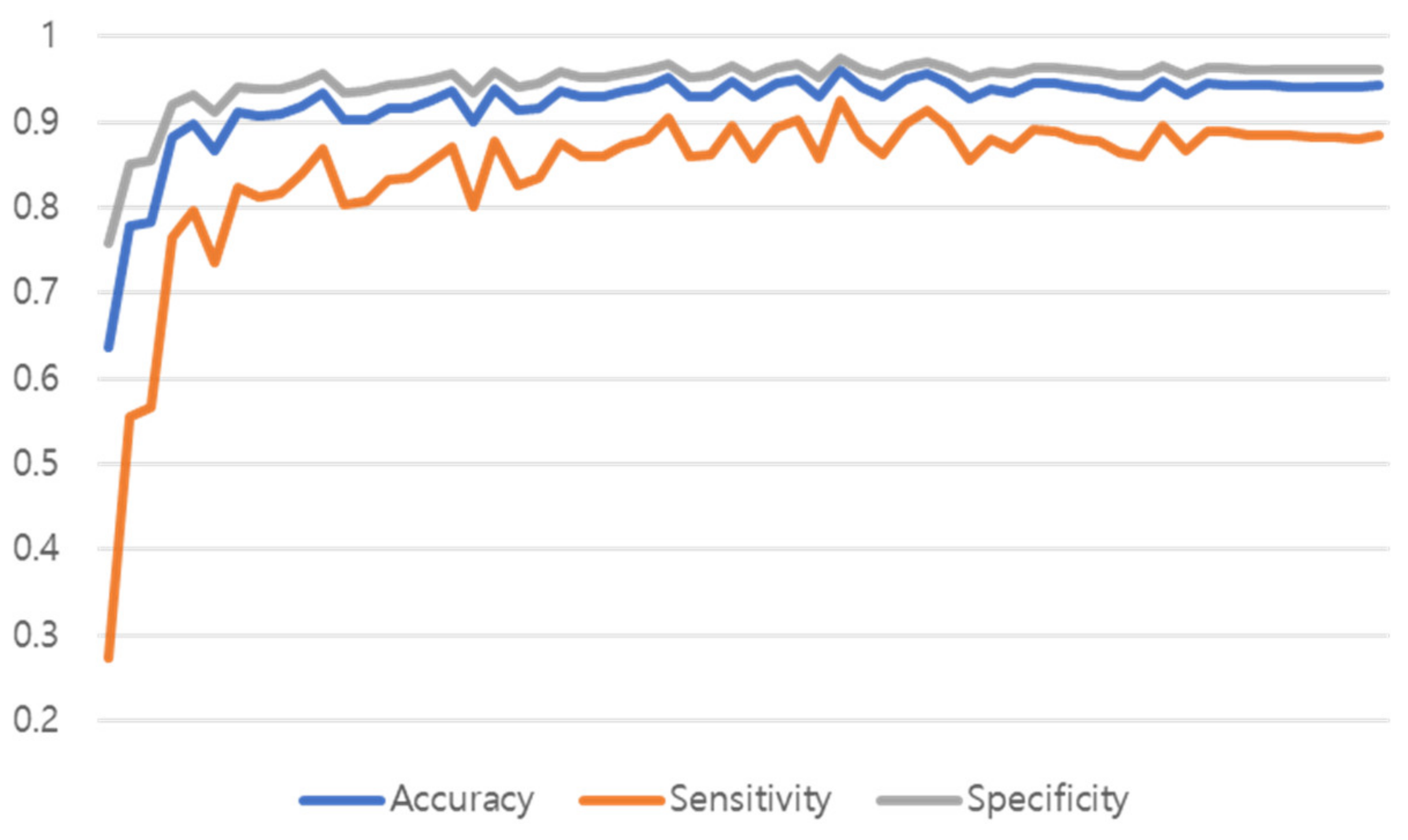
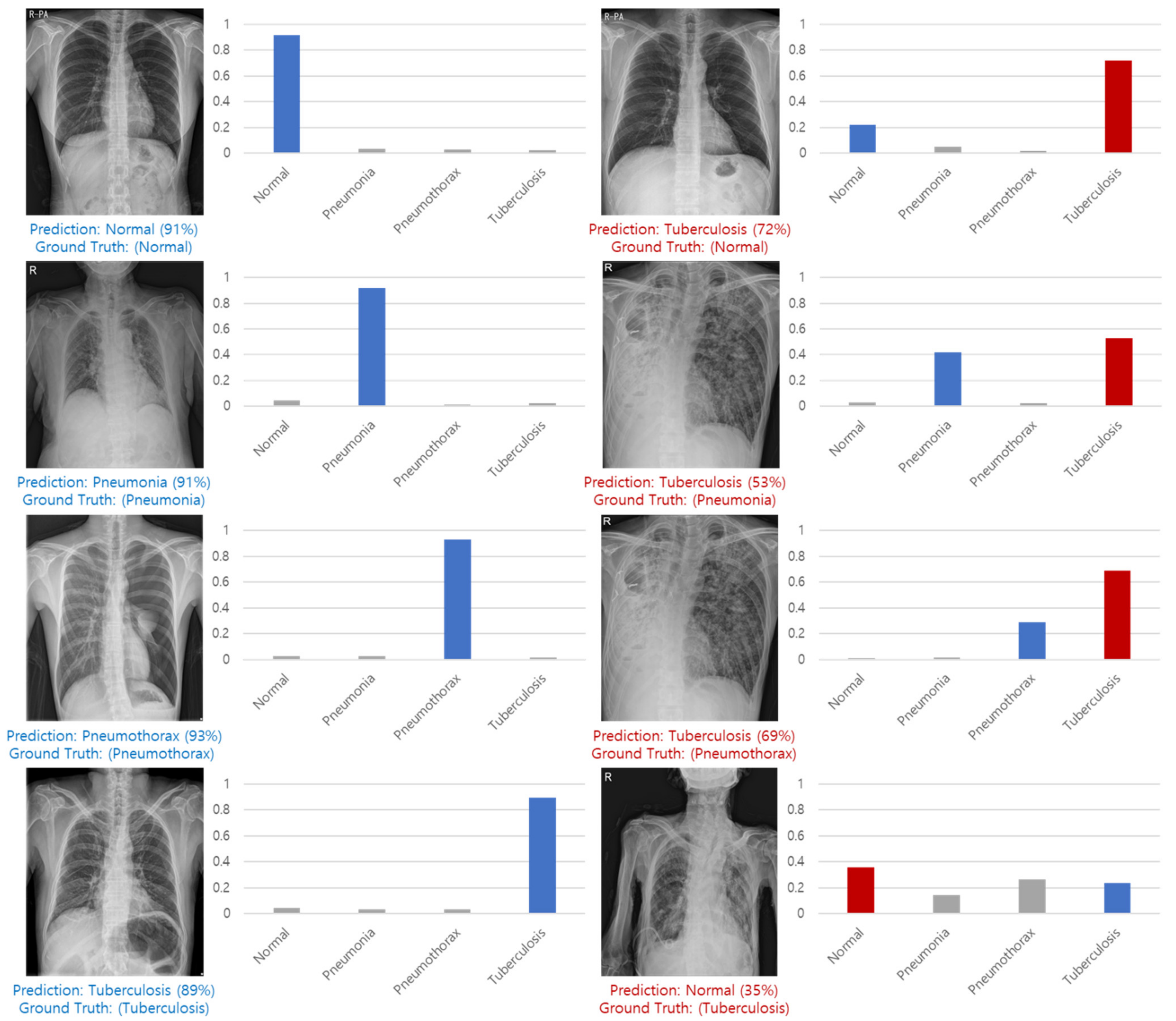
Figure 15 shows the training graph of the model that predicted Normal, Pneumonia, Pneumothorax, and Tuberculosis by learning 51,866 de-identified images provided by Soonchunhyang University Hospital, Cheonan. The performance was measured with a single model to which both the proposed preprocessing and multi GAP were applied, and the performance of the test set was measured in the epoch that had the highest validation accuracy performance. Figure 16 shows examples of correct predictions and incorrect predictions by classes.

As a result of learning all 60 epochs, the 35 epochs showed the highest performance, and the validation performance of the 35 epochs was shown in

Table 12. Validation Performance.

	Accuracy	Sensitivity	Specificity
Total	96.22%	92.45%	97.48%

. As a result of measuring the performance of the test set, the test performance and inference time are shown in

Table 13. Test Performance.

	Accuracy	Sensitivity	Specificity
Normal	98.80%	97.30%	99.30%
Pneumonia	93.50%	87.10%	95.63%
Pneumothorax	98.45%	96.70%	99.03%
Tuberculosis	93.65%	87.70%	95.63%
Total	96.10%	92.20%	97.40%

and

Table 14. Test Inference Time.

	Inference Time
Total	13 m
Average	0.2 s

.

9. Conclusions

In this study, we proposed a multi-class classification method of lung disease using CNN model. After making the image in a 1:1 ratio and center cropping it by 87.5%, a classification model of the Multi GAP format was created based on the Noisy Student ImageNet Pretrained weight of the EfficientNet B7 model. In the NIH dataset for benchmarks measurement when lung disease was predicted with the model, the models to which the proposed method was applied showed high performance at 84.86%, 85.15%, and 85.32% of the accuracy criteria, and the model to which all the suggestions were applied showed the most satisfactory performance. Shown in the dataset of Soonchunhyang University Hospital in Cheonan, which includes tuberculosis, an average of 96% accuracy, an average sensitivity of 92.20, and an average specificity of 97.40% were obtained. The average test inference time was 0.2 s, and as a result of not much difference between the validation performance and the test performance, it was confirmed that the generalization of the model was not bad.

Chest X-ray is the basis of all chest radiographic tests, and it is easy to check the overall outline of the chest at a glance, and it is suitable for follow-up examination because it is easy to observe the chest disease changes. However, there is also a disadvantage that accurate reading of chest X-ray is difficult due to the complex anatomical structure of the chest. Clinical decision supporting system (CDSS) is a system that helps clinicians make clinical decisions, and is a set of programs that help with more precise diagnosis or prevent misdiagnosis. Therefore, our multi-class classification method of lung disease using CNN model showed high performance (Accuracy, 96.22: Sensitivity, 92.45: Specificity, 97.48) and could be considered applicable to CDSS system for lung diseases.

Future research intends to proceed with learning methods for more diverse disease types and methods for improving learning performance.

References

- Hinton, G.E.; Osindero, S.; Teh, Y.W. A fast learning algorithm for deep belief nets. Neural Comput. 2006, 18, 1527–1554. [Google Scholar] [CrossRef] [PubMed]
- Bengio, Y.; Lamblin, P.; Popovici, D.; Larochelle, H. Greedy layer-wise training of deep networks. In Proceedings of the Advances in Neural Information Processing Systems, Vancouver, BC, Canada, 3–8 December 2007; pp. 153–160. [Google Scholar]
- LeCun, Y.; Boser, B.; Denker, J.S.; Henderson, D.; Howard, R.E.; Hubbard, W.; Jackel, L.D. Backpropagation applied to handwritten zip code recognition. Neural Comput. 1989, 1, 541–551. [Google Scholar] [CrossRef]
- Krizhevsky, A.; Sutskever, I.; Hinton, G.E. Imagenet classification with deep convolutional neural networks. Adv. Neural Inf. Process. Syst. 2012, 25, 1097–1105. [Google Scholar] [CrossRef]
- Simonyan, K.; Zisserman, A. Very deep convolutional networks for large-scale image recognition. arXiv 2014, arXiv:1409.1556. [Google Scholar]
- He, K.; Zhang, X.; Ren, S.; Sun, J. Deep residual learning for image recognition. In Proceedings of the IEEE Conference on Computer Vision and Pattern Recognition, Las Vegas, NV, USA, 27–30 June 2016; pp. 770–778. [Google Scholar]
- Szegedy, C.; Liu, W.; Jia, Y.; Sermanet, P.; Reed, S.; Anguelov, D.; Erhan, D.; Vanhoucke, V.; Rabinovich, A. Going deeper with convolutions. In Proceedings of the IEEE Conference on Computer Vision and Pattern Recognition, Boston, MA, USA, 7–12 June 2015; pp. 1–9. [Google Scholar]
- Papers with Code: The latest in Machine Learning, Browse State-of-the-Art Image Classification. Available online: https://paperswithcode.com/task/image-classification (accessed on 4 January 2021).
- Park, S.; Jeong, W.; Moon, Y.S. X-ray Image Segmentation using Multi-task Learning. KSII Trans. Internet Inf. Syst. (TIIS) 2020, 14, 1104–1120. [Google Scholar]
- Ming, J.; Yi, B.; Zhang, Y.; Li, H. Low-dose CT image denoising using classification densely connected residual network. KSII Trans. Internet Inf. Syst. (TIIS) 2020, 14, 2480–2496. [Google Scholar]
- Hao, R.; Qiang, Y.; Liao, X.; Yan, X.; Ji, G. An automatic detection method for lung nodules based on multi-scale enhancement filters and 3D shape features. KSII Trans. Internet Inf. Syst. (TIIS) 2019, 13, 347–370. [Google Scholar]
- American Lung Association, Learn About Pneumonia. Available online: https://www.lung.org/lung-health-diseases/lung-disease-lookup/pneumonia/learn-about-pneumonia (accessed on 20 February 2021).
- American Lung Association, Learn About Pneumothorax. Available online: https://www.lung.org/lung-health-diseases/lung-disease-lookup/pneumothorax/learn-about-pneumothorax (accessed on 20 February 2021).
- American Lung Association, Learn About Tuberculosis. Available online: https://www.lung.org/lung-health-diseases/lung-disease-lookup/tuberculosis/learn-about-tuberculosis (accessed on 20 February 2021).
- Gabruseva, T.; Poplavskiy, D.; Kalinin, A. Deep learning for automatic pneumonia detection. In Proceedings of the IEEE/CVF Conference on Computer Vision and Pattern Recognition Workshops, Virtual Conference, 14–19 May 2020; pp. 350–351. [Google Scholar]
- Ibrahim, A.U.; Ozsoz, M.; Serte, S.; Al-Turjman, F.; Yakoi, P.S. Pneumonia classification using deep learning from chest X-ray images during COVID-19. Cogn. Comput. 2021, 1–13. [Google Scholar] [CrossRef]
- Loddo, A.; Pili, F.; Di Ruberto, C. Deep Learning for COVID-19 Diagnosis from CT Images. Appl. Sci. 2021, 11, 8227. [Google Scholar] [CrossRef]
- NIH Chest X-ray Dataset. Available online: https://cloud.google.com/healthcare/docs/resources/public-datasets/nih-chest (accessed on 4 January 2021).
- Tan, M.; Le, Q. Efficientnet: Rethinking model scaling for convolutional neural networks. In Proceedings of the International Conference on Machine Learning, Long Beach, CA, USA, 9–15 June 2019; pp. 6105–6114. [Google Scholar]
- Lin, T.Y.; Dollár, P.; Girshick, R.; He, K.; Hariharan, B.; Belongie, S. Feature pyramid networks for object detection. In Proceedings of the IEEE Conference on Computer Vision and Pattern Recognition, Honolulu, HI, USA, 21–26 July 2017; pp. 2117–2125. [Google Scholar]
- Cubuk, E.D.; Zoph, B.; Shlens, J.; Le, Q.V. Randaugment: Practical automated data augmentation with a reduced search space. In Proceedings of the IEEE/CVF Conference on Computer Vision and Pattern Recognition Workshops, Seattle, WA, USA, 14–19 June 2020; pp. 702–703. [Google Scholar]
- Montalbo, F.J.P. A Computer-Aided Diagnosis of Brain Tumors Using a Fine-Tuned YOLO-based Model with Transfer Learning. KSII Trans. Internet Inf. Syst. 2020, 14, 4816–4834. [Google Scholar]
- Deng, J.; Dong, W.; Socher, R.; Li, L.J.; Li, K.; Fei-Fei, L. Imagenet: A large-scale hierarchical image database. In Proceedings of the 2009 IEEE Conference on Computer Vision and Pattern Recognition, Miami, FL, USA, 20–25 June 2009; pp. 248–255. [Google Scholar]
- Xie, Q.; Luong, M.T.; Hovy, E.; Le, Q.V. Self-training with noisy student improves imagenet classification. In Proceedings of the IEEE/CVF Conference on Computer Vision and Pattern Recognition, Virtual Conference, 14–19 May 2020; pp. 10687–10698. [Google Scholar]
- Zhang, M.R.; Lucas, J.; Hinton, G.; Ba, J. Lookahead optimizer: K steps forward, 1 step back. arXiv 2019, arXiv:1907.08610. [Google Scholar]
- Dozat, T. Technical report, Incorporating Nesterov Momentum into Adam. In Proceedings of the ICLR Workshop, San Diego, CA, USA, 7–9 May 2015. [Google Scholar]
- Kingma, D.P.; Ba, J. Adam: A method for stochastic optimization. arXiv 2014, arXiv:1412.6980. [Google Scholar]
- Botev, A.; Lever, G.; Barber, D. Nesterov’s accelerated gradient and momentum as approximations to regularised update descent. In Proceedings of the 2017 International Joint Conference on Neural Networks (IJCNN), Anchorage, AK, USA, 14–19 May 2017; pp. 1899–1903. [Google Scholar]
- Goyal, P.; Dollár, P.; Girshick, R.; Noordhuis, P.; Wesolowski, L.; Kyrola, A.; Tulloch, A.; Jia, Y.; He, K. Accurate, large minibatch sgd: Training imagenet in 1 hour. arXiv 2017, arXiv:1706.02677. [Google Scholar]
- Loshchilov, I.; Hutter, F. Sgdr: Stochastic gradient descent with warm restarts. arXiv 2016, arXiv:1608.03983. [Google Scholar]
- Müller, R.; Kornblith, S.; Hinton, G. When does label smoothing help? arXiv 2019, arXiv:1906.02629. [Google Scholar]
- Nishikawa, S.; Yamada, I. Studio Ousia at the NTCIR-15 SHINRA2020-ML Task. In Proceedings of the NTCIR 15 Conference: Proceedings of the 15th NTCIR Conference on Evaluation of Information Access Technologies, Tokyo, Japan, 8–11 December 2020. [Google Scholar]
Figure 1.
Forecast of the size of the healthcare market in Korea (KISTI Market Report).
Figure 2.
Classification, detection, and segmentation task.
Figure 3.
Center cropped image after processing in a 1:1 ratio.
Figure 4.
(a) Baseline. (b) Width Scaling. (c) Depth Scaling. (d) Resolution Scaling.
Figure 5.
Single Feature Map and Feature Pyramid Network.
Figure 6.
Encoder with Concat structure.
Figure 7.
Full model structure.
Figure 8.
Drop Connect and Drop Out.
Figure 9.
Undersampling and Oversampling methods.
Figure 10.
X-ray image with Rand Augment applied.
Figure 11.
Update method of Lookahaed, Adam, and Nadam.
Figure 12.
Learning Rate Curve.
Figure 13.
Confusion Matrix.
Figure 14.
NIH dataset training graph.
Figure 15.
SCH dataset training graph.
Figure 16.
Correct predictions and incorrect predictions by classes.