Article

A Feasibility Study for a Nonlinear Guided Wave Mixing Technique

1
Extreme Environment Design and Manufacturing Engineering, Changwon National University, Changwon 51140, Korea
2
Equipment Innovation Team, TSP Center, Samsung Electronics, Asan 31489, Korea
3
School of Mechanical Engineering, Changwon National University, Changwon 51140, Korea
*
Author to whom correspondence should be addressed.
Appl. Sci. 2021, 11(14), 6569; https://doi.org/10.3390/app11146569
Submission received: 2 June 2021 / Revised: 1 July 2021 / Accepted: 14 July 2021 / Published: 16 July 2021
(This article belongs to the Special Issue Applications on Ultrasonic Wave ‖)

Abstract

:
Ultrasonic non-destructive testing is an effective means of examining objects without destroying them. Among such testing, ultrasonic nonlinear evaluation is used to detect micro-damage, such as corrosion or plastic deformation. In terms of micro-damage evaluation, the data that comes from amplitude comparison in the frequency domain plays a significant role. Its technique and parameter are called ultrasonic nonlinear technique and nonlinearity. A certain portion of nonlinearity comes from the equipment system, while the other portion of nonlinearity comes from the material. The former is system nonlinearity, while the latter is material nonlinearity. System nonlinearity interferes with interpretation, because its source is not from the material. In this study, in order to minimize system effects, a mixing technique is implemented. To use the large area inspection ability of the guided wave, the main research issue in this paper is focused on the guided wave mixing technique. Moreover, several bulk wave mixing theory equations become good concepts for guided wave mixing theoretical study, and the conventional nonlinear technique and guided wave mixing experimental results are compared in this study to confirm the reliability. This technique can play an important role in quantitatively discriminating fine damage by minimizing the nonlinearity of the equipment system.

1. Introduction

Ultrasonic waves and radiation are normally used for non-destructive testing. In the case of ultrasonic testing, the velocity, time, and distance of ultrasonic waves help the user to find defects. However, these simple parameters do not satisfy all evidence for evaluating micro-damage in a material, such as damage from corrosion, plastic deformation, or microstructure variation. The estimation ability of nonlinear information in the frequency domain also needs to be improved.
In ultrasonic nonlinear techniques, it is important to measure the second harmonic component. The ratio between the primary and secondary harmonic wave amplitudes becomes the nonlinear parameter called nonlinearity. Based on the nonlinearity derived from the second harmonic component, many research results have been widely studied for micro-damage assessments [1,2,3]. Even though nonlinearity indicates good micro-damage assessment sensitivity, it usually shows relative results. One of the main reasons that it shows relative results is that the nonlinearity is affected by the experimental setup. A certain portion of nonlinearity comes from the system, which includes the equipment, sensors, and cables. As such, nonlinearity influenced by the system acts as an error. This means that reducing system nonlinearity could increase the accuracy of the results. One of the few techniques that can reduce system nonlinearity is the wave mixing technique [4]. Currently, many researchers are researching a nonlinear method to measure the third harmonic ratio, but the third harmonic has a very small relative ratio, so many variables exist, and as such it is difficult to apply in practical applications, and theoretical and experimental verification is being performed [5,6].
There are two reasons why the mixing technique could minimize the system nonlinearity. The first reason is that the key point of the wave mixing technique is that one mixing wave is generated from two primary waves. In contrast to conventional ultrasonic nonlinear techniques, the received signal does not come directly from the equipment, which thus does not influence the mixing signal much. In the words, the mixing technique has less system nonlinearity [7]. The second reason is that mixing techniques are classified into two types depending on the frequency, or the sum or difference of the primary wave frequencies. Theoretically, each primary wave signal produces the same or similar system nonlinearity. If the mixing signal were to have the difference of the primary wave frequencies, the system nonlinearity would theoretically be canceled out [7,8].
Mixing technique theory has been studied for a long time, but there are not as many experimental studies as theoretical studies. Jones et al. [8] and Taylor et al. [9] developed a theoretical mixing basement. Based on basic equations, wave mixing terms and information are derived. The major features of its study consider equations to contain linear and nonlinear information. The main factors include the interaction angle and mixing signal propagation. Hu, L. et al. [10] numerically analyzed the one-way mixing of S0 and A0 modes using simulation, and Bin, W. et al. [11] detected micro-defects with nonlinear mixing experiments and simulations in S0 single mode. Croxford et al. [7] measured the material nonlinearity using a non-collinear mixing technique, conducting experiments on large and thick specimens. Moreover, Liu et al. [4] theoretically and experimentally studied a collinear mixing technique. Recently, research to study nonlinearity by constructing four-wave mixing (FWM) using highly nonlinear fiber (Bi-HNLF) and laser has also been actively conducted [12,13].
All researchers mentioned in this paper have tried to reduce the system influence on the results. However, these studies were limited to bulk waves, and guided wave mixing has not been studied as much, because guided waves have a dispersive characteristic [14,15,16,17,18]. Nonetheless, guided waves are more appropriate than bulk waves for scanning large areas such as plates and long pipes. In addition, previous researchers have conducted guided wave mixing studies in a single mode [19,20,21,22]. Representatively, Adachi, T. et al. [23] numerically and experimentally shows the non-collinear mixing of low-order asymmetric Rayleigh-Lamb waves in the SH0 single mode. Guided waves have various modes, and the experimental results vary greatly depending on the mode selection and the angle of incidence. Therefore, the guided wave mixing technique deserves study [24,25,26,27,28,29].
In this study, guided wave mixing was theoretically analyzed and experimentally verified. To use bulk wave mixing theory and overcome the difficulty of interpreting guided waves with different modes and frequencies, several assumptions are applied. Several assumptions help guided wave displacement components (in-plane and out-of-plane displacement) be treated as longitudinal and transverse waves. The guided wave mixing and the conventional ultrasonic nonlinear technique are compared by using the same specimen. The significant contents in this study are as follows:
  • Based on bulk wave mixing theory and several assumptions, guided wave mixing technique is studied theoretically.
  • Based on theoretical study, an experimental test is conducted. Both the available mixing condition and non-available mixing condition are experimented with.
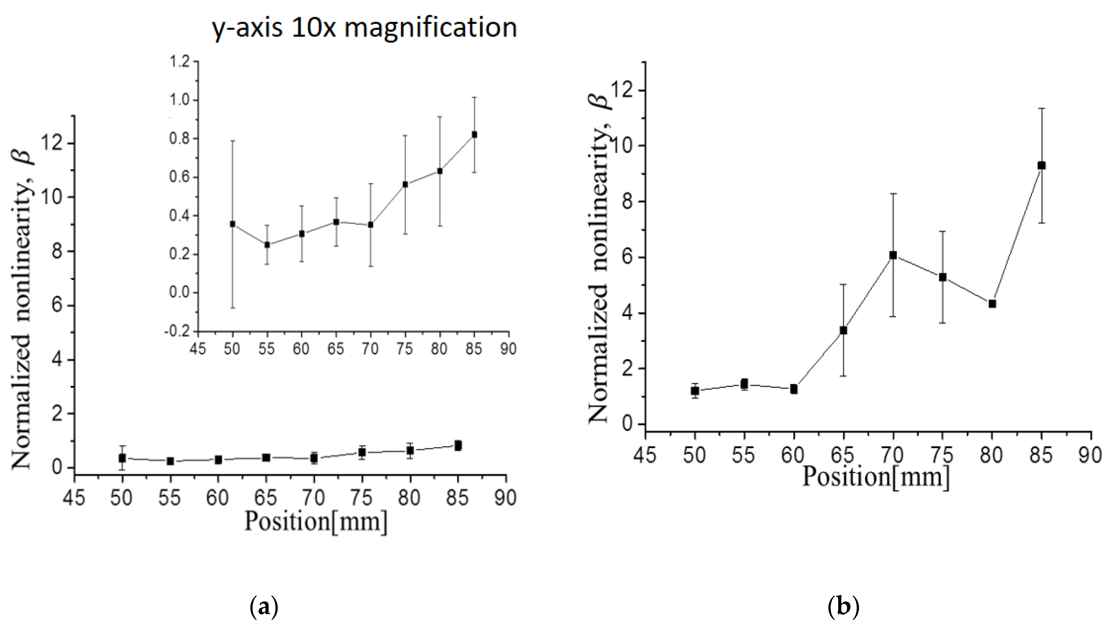
  • As the distance is changed, nonlinearity is measured by the conventional technique and the guided wave mixing technique for comparison.

2. Theory

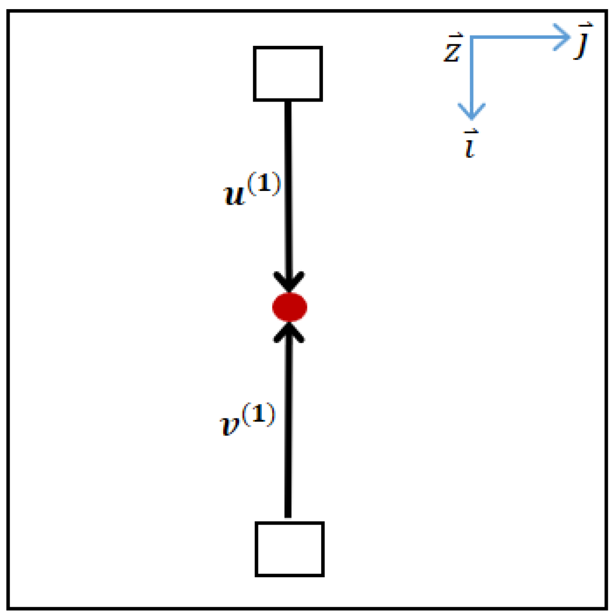
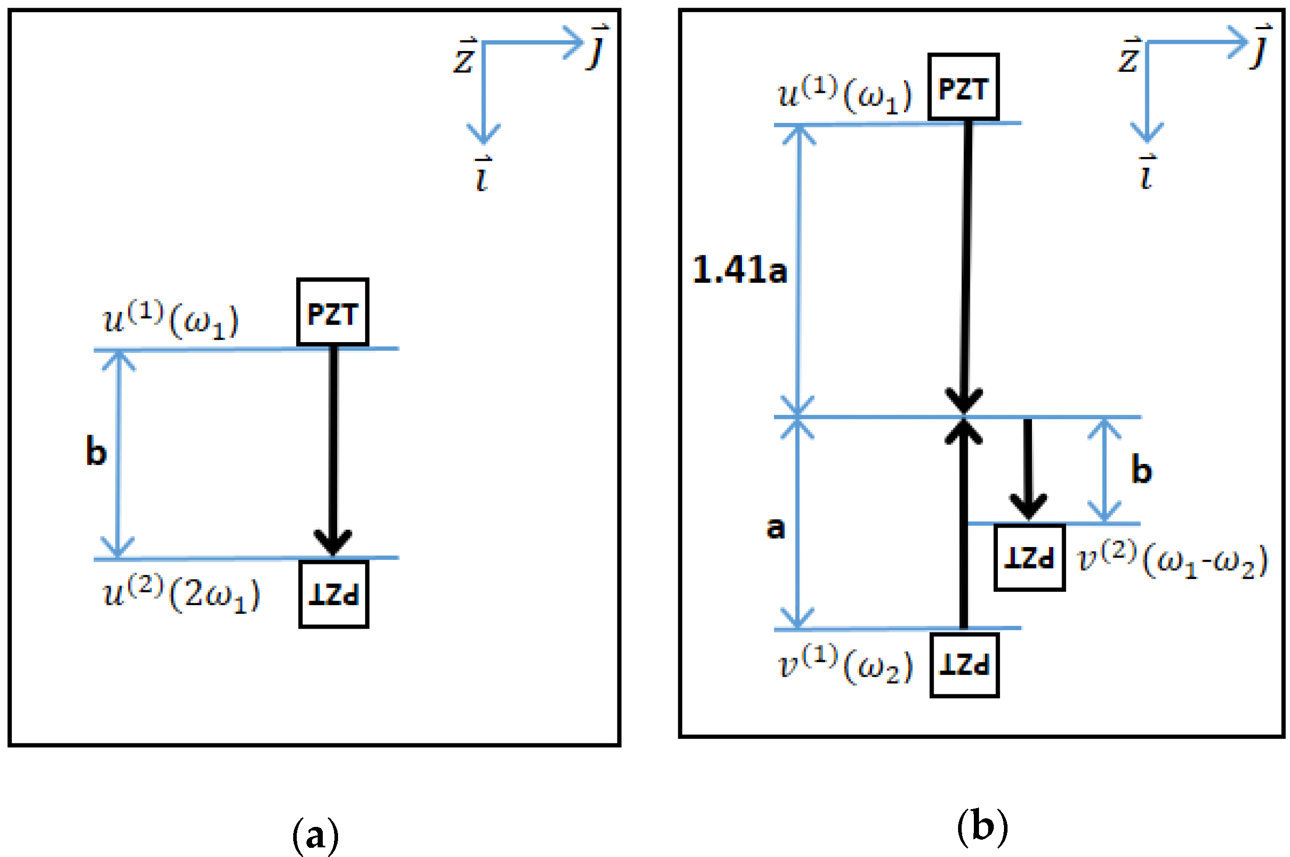
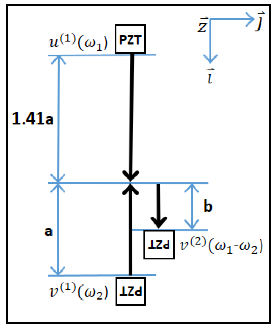
2.1. Guided Wave Mixing Theory

A bulk wave consists of a longitudinal wave and transverse wave, and has the same velocity, regardless of frequency. The characteristics of bulk waves make studying and applying them easy. Guided wave study is more difficult to use for experiments. The most important feature of a guided wave is dispersion. The wave velocity has a variety of value ranges that depend on the mode and frequency, and the specimen depth makes the magnitude of displacement different.
Guided wave displacement consists of in-plane displacement ( u 1 ) , and out-of-plane displacement   ( u 3 ) . In-plane displacement takes place horizontal to the propagation direction, while out-of-plane displacement takes place vertical to that direction. Figure 1 shows the in-plane and out-of-plane placement coordinate diagram. In the figure, x and t denote the propagation direction and thickness, respectively. These components are expressed in Equations (1) and (2) [30,31]. These indicate scalar potential ( φ ) and vector potential ( ψ ), as in Equation (3). This is called Helmholtz decomposition. Equations (1) and (2) can be simplified into Equations (4) and (5):
u 1 = ( ϕ x 1 + φ 2 x 3 ) = ( i k Φ ( x 3 ) + x 3 ( Ψ ( x 3 ) ) ) exp ( i ( k x 1 ω t ) )
u 3 = ( ϕ x 3 φ 2 x 1 ) = ( x 3 ( Φ ( x 3 ) ) i k Ψ ( x 3 ) ) exp ( i ( k x 1 ω t ) )
u = ϕ + × φ
u 1 ( 1 ) = A 1 exp i ( k 1 x ω 1 t )
u 3 ( 1 ) = A 2 exp i ( k 3 x ω 1 t )
where, k and ω are the wave vector and frequency, respectively, and A shows the positive wave amplitude.
In the bulk wave, the longitudinal component is horizontal to the propagation direction, while the transverse component is vertical to the propagation direction. This concept becomes equivalent to the in-plane and out-of-plane displacement of the guided wave. These displacement components cannot be separated out in one guided wave signal, but the ratio of the two components changes with the mode and frequency. Analyzing wave structure helps to determine the component ratio.
u t t c l 2 u a a = ( 3 c l 2 + C 111 / ρ ) u a u a a + ( c l 2 + C 166 / ρ ) ( v a v a a + w a w a a )
v t t c s 2 v a a = ( c l 2 + C 166 / ρ ) ( u a v a a + v a u a a )
w t t c s 2 w a a = ( c l 2 + C 166 / ρ ) ( u a w a a + w a u a a )
u ( 1 ) = A sin ( k l x ω l t )
v ( 1 ) = B sin ( k s x + ω s t )
where, C 111 and C 116 indicate the third order elastic moduli, and c l and c s indicate the longitudinal and transverse wave’s velocities respectively. ρ denotes the constant density. Subscripts   a and t mean the spatial coordinate and time, and ‘(1)’ indicates primary waves.
Some conditions are assumed to use some parts of bulk wave mixing theory in guided wave mixing theory. If the in-plane displacement is greater than the out-of-plane displacement, the guided wave signal is treated as a longitudinal wave. If the out-of-plane displacement is greater, the signal is treated as a transverse wave in this paper.
Figure 2 illustrates the guided wave mixing concept. The case in which one component has dominant in-plane displacement, and another component has dominant out-of-plane displacement, is shown in the plate. Each signal is defined by Equations (9) and (10). These are input primary waves in this mixing theory study. Because the directions show opposite, the marks inside of the sine functions in Equations (9) and (10) are different. Moreover, Equations (6)–(8) express nonlinear wave equations (Goldberg, 1961) [32]. These nonlinear wave equations represent wave behavior in nonlinear conditions. The nonlinearity ( β s ) is defined as β s = ( c l 2 + C 166 / ρ ) . Based on these derived equations and two input primary waves (Equations (9) and (10)), mixing wave components can be derived.
Equation (11) can be derived by substituting two primary waves based on Equations (9) and (10) in Equation (7). After a few rearrangement steps, Equation (12) is obtained. Here, there are two out-of-plane dominant mixing waves. The frequency of the first one is the difference of the two primary wave frequencies ( ω 1 ω 2 ) , while that of the second one is the sum ( ω 1 + ω 2 ) . The point of interest is the difference-frequency mixing signal for dominant out-of-plane displacement, so the sum-frequency component is ignored.
v t t ( 2 ) c s 2 v a a ( 2 ) = β s ( A B k l k s 2 cos ( k l x ω l t ) sin ( k s x + ω s t ) + A B k l 2 k s sin ( k l x ω l t ) cos ( k s x + ω s t ) )
v t t ( 2 ) c s 2 v a a ( 2 ) = β s ( 1 2 A B k l k s ( k l + k s ) sin ( ( k l + k s ) x ( ω 1 ω s ) t ) + 1 2 A B k l k s ( k l k s ) sin ( ( k l k s ) x ( ω l + ω s ) t ) )
After perturbation method processes and several steps, the final form of the mixing component is expressed as Equation (13) [33,34]. It contains the difference frequency of primary waves. One in-plane dominant wave is mixed with the other one out-of-plane dominant wave to generate an out-of-plane dominant mixing signal with the difference of the primary waves’ frequencies: u ( ω 1 ) + v ( ω 2 ) v ( ω 1 ω 2 ) . Whether the propagation direction is the same as that of a longitudinal component defined can be determined by checking the mark in the sine function of Equation (13). Figure 3 explains this.
Equation (14) shows the amplitude term of a mixing signal (Equation (13)). Even though the concept of the mixing technique is similar to second harmonic generation, experimental signal detection is much more difficult. A few considerations are therefore needed to detect a mixing signal.
v ( 2 ) = C sin ( ( k l + k s ) x ( ω l ω s ) t )
C = 1 2 β s A B k l k s ( k l + k s ) ( ω l ω s ) 2 + c s 2 ( k l + k s ) 2
ω s ω l = c 1 c 2 2 c 1 = c l c s 2 c l
Figure 3. Guided wave mixing concept with mixing signal in a plate.
Applsci 11 06569 g003
The mixing signal amplitude (Equation (14)) is a function of the primary wave frequencies. Additionally, when the denominator becomes zero, the value becomes infinite. Based on these concepts, the primary wave frequencies are decided. Equation (15) denotes the frequency ratio for the theoretical maximum amplitude. If a specimen is set, the longitudinal and transverse wave velocities are constants, because longitudinal and transverse wave velocities are determined by the material property. Therefore, their ratio is also constant.
For an aluminum specimen (Al1050), the longitudinal and transverse wave velocities are (6.36 and 3.01) mm/µs, respectively. The frequency ratio that results in the maximum mixing wave amplitude is ω s / ω l = 0.263, which is simplified as: u ( ω 1 ) + v ( 0.263 ω 1 ) v ( 0.737 ω 1 ) .

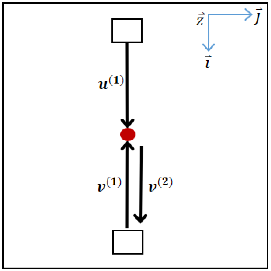
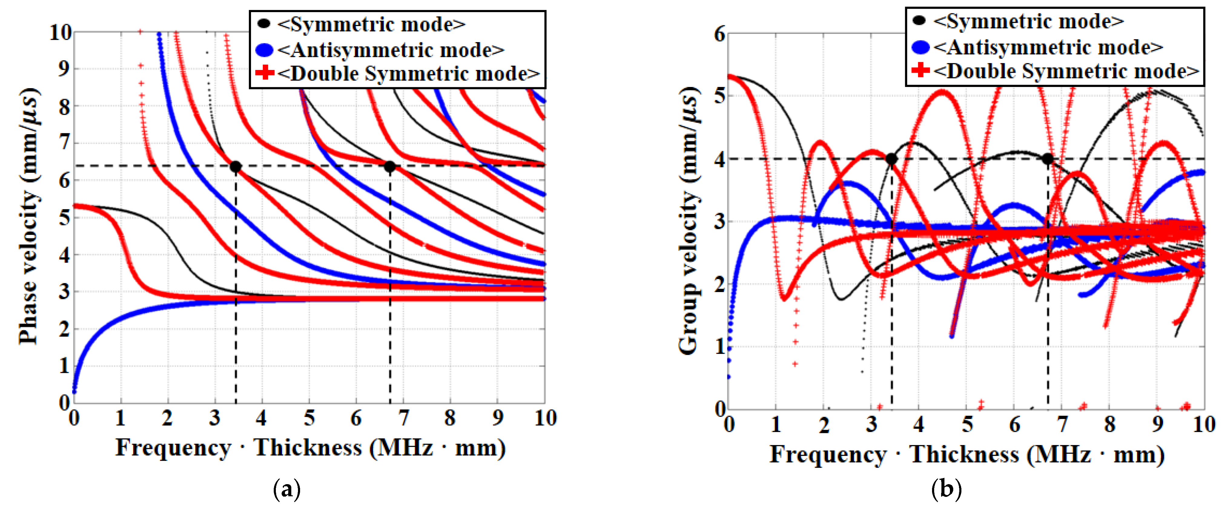
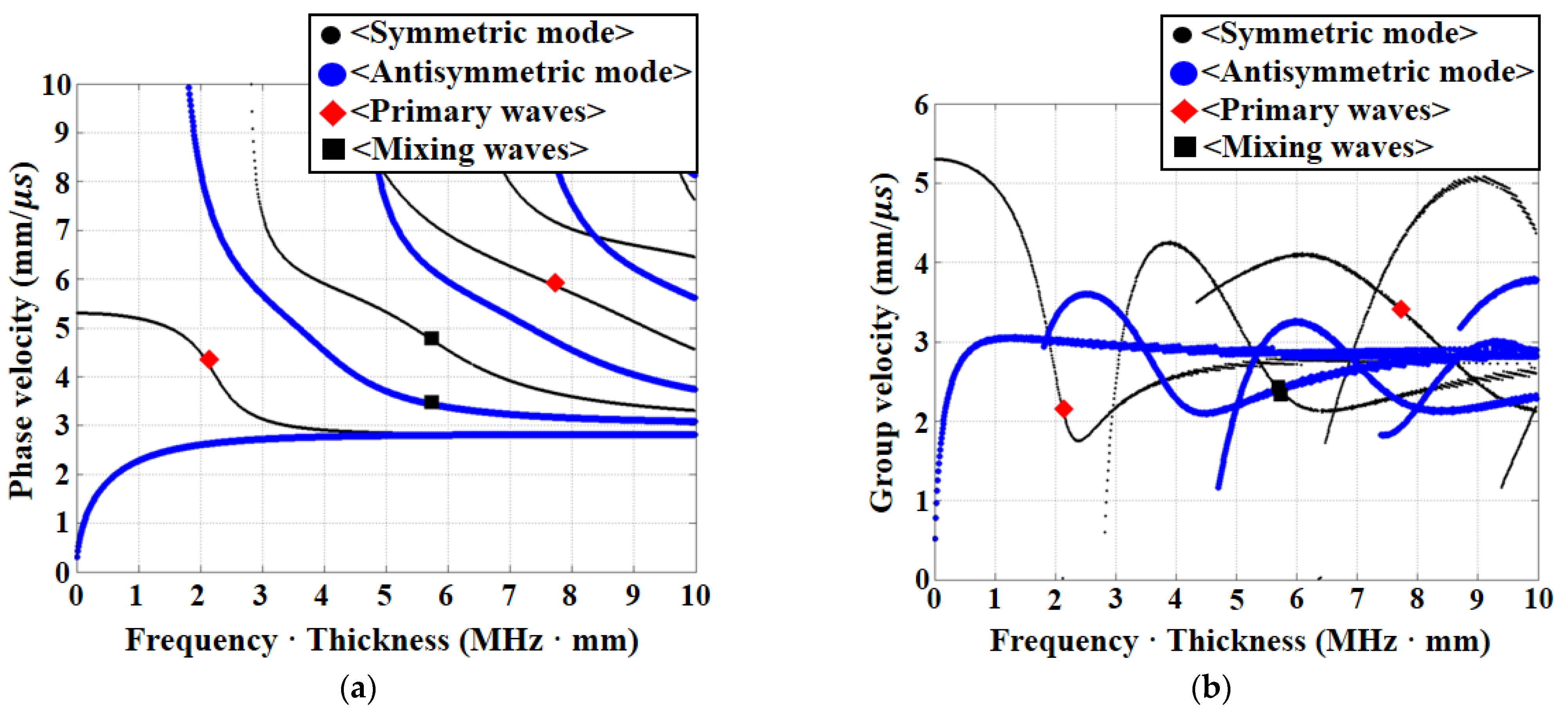
2.2. Phase Matching Mode Theory

The phase matching mode technique is normally used for measuring guided wave nonlinearity in a plate. The most important phenomenon of nonlinearity is the second harmonic wave. Generally, its signal has double the frequency of the primary wave. In a bulk wave, the primary wave velocity is the same as the second harmonic wave velocity. Therefore, the two components arrive at the same time, so measuring the bulk wave nonlinearity becomes simple. However, in a guided wave, the two components have different velocities because of the dispersion characteristic. This makes studying nonlinear guided waves difficult. Because the arrival times of the two components are different, signal reception at the same position is almost impossible. However, fortunately there are a few mode cases where the primary and second harmonic wave velocities are equal. This combined mode and frequency is called the phase matching mode [35]. Based on the phase matching mode, nonlinearity measurement could be conducted in a plate or pipe using guided waves.
Equations (16) and (17) shows the symmetric mode equation and double frequency harmonic symmetric mode equation, respectively. Equation (17) represents the second harmonic component. k and h mean the wave number and half of plate thickness respectively. In this study, only the symmetric mode is considered for the phase matching mode experiment. Here, p and q are given by p 2 = ( ω / c l ) 2 k 2 and q 2 = ( ω / c s ) 2 k 2 . Figure 4a shows the phase velocity dispersion curves, while Figure 4b shows the group velocity dispersion curve based on Equations (16) and (17) for aluminum (Al 1050):
tan ( q h ) tan ( p h ) = 4 k 2 p q ( k 2 q 2 ) 2
tan ( 2 q h ) tan ( 2 p h ) = 4 k 2 p q ( k 2 q 2 ) 2
One example of phase matching mode is the component with 3.4 MHz frequency and S1 mode, and the second harmonic wave with 6.8 MHz frequency and S2 mode. Both frequency components are the intersection point (black circle) of each dashed line in Figure 4a,b. These two components have the same phase velocity and group velocity. The phase matching mode concept was studied by Deng et al. [35]. Experimental application of the phase matching mode was studied by Li et al. [36].

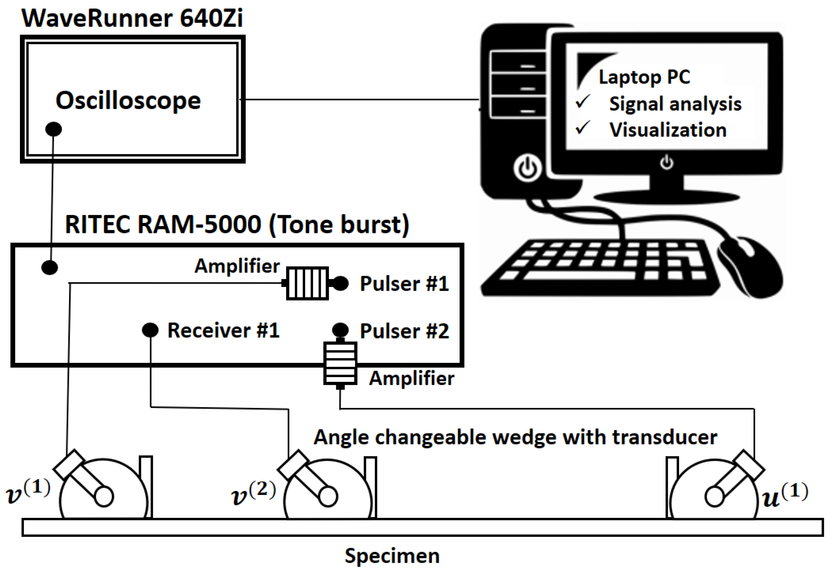
3. Experimental Setup

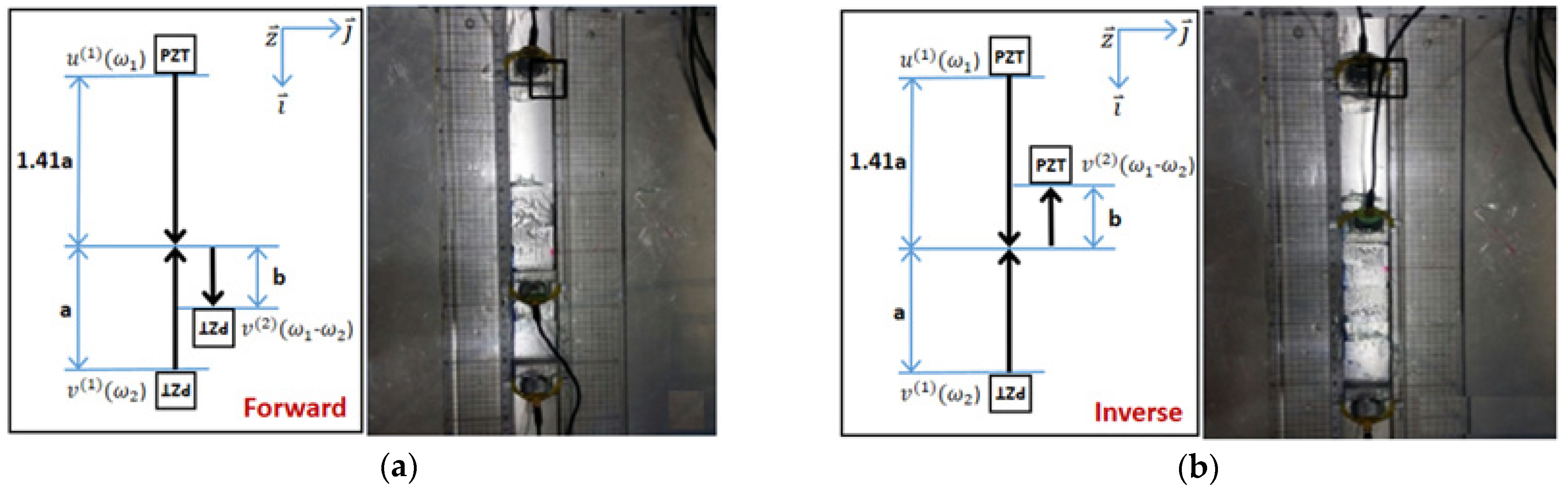
3.1. Experimental Setup for Guided Wave Mixing Generation

A guided wave mixing signal was generated using an aluminum specimen (Al 1050). The specimen thickness is 1 mm. The main purpose of this experiment is to generate an out-of-plane dominant mixing signal from one in-plane dominant signal and one out-of-plane dominant signal. Table 1 shows the primary wave frequencies and modes that are decided based on Equation (18). The primary waves consist of an in-plane-dominant wave (7.83 MHz, S2) and out-of-plane dominant wave (2.06 MHz, S0). In Table 1 and Table 2, in order to express the relative magnitude between in-plane and out-of-plane displacement, alphabet letters a ,   b ,   c ,   d are used. Without this object, a ,   b ,   c ,   d do not have any other means.
u ( ω 1 ) + v ( 0.263 ω 1 ) = v ( 0.737 ω 1 ) u ( 7.83   MHz ) + v ( 2.06   MHz ) v ( 5.77   MHz )  
In the dispersion curve, several modes exist at 5.77 MHz that are mixing waves. However, there are only two out-of-plane dominant modes: S1 and A1 (Table 2). Both mixing signals have the possibility of becoming wave mixing signals. Figure 5a,b show the dispersion curves with the primary waves (Red diamond) and mixing waves (Black square). Figure 6 shows the basic sensor arrangement. To mix the two primary waves, each sensor distance is set differently. The quantity b indicates the propagation distance of the mixing signal from the mixing point. The experimental setup is configured as shown in Figure 7. The pulser and receiver use RITEC co.’s RAM-5000 and generate a sine wave. Pulser #1 and #2 are used with amplifiers installed, and the received signal can be verified with an oscilloscope. RAM-5000 has two pulsers and two receivers and is actively used in ultrasonic mixing experiments. Each sensor was tested using an Olympus’s sensor.
The mixing signal propagation direction was calculated for the two possible modes. Figure 8 shows four experimental setups with different modes and propagation directions. The distances of the sender and receiver sensors are defined as a = 100 mm and |b| = 20 mm.
1 : u ( 6.83   MHz ) + v ( 2.06   MHz ) v ( 4.77   MHz ) 2 : u ( 7.83   MHz ) + v ( 2.06   MHz ) v ( 5.77   MHz ) 3 : u ( 8.83   MHz ) + v ( 2.06   MHz ) v ( 6.77   MHz )
Equation (19) represents the frequency combination for the experiment. The second part of Equation (19) has exactly the same equation as Equation (18), and maximizes the mixing signal amplitude. The first and third frequency combinations have different calculated frequency ratios. These two ratios were implemented to find whether a mixing signal is detected at only the calculated frequency ratio. The second frequency setup is applied to the four experimental setups with different modes and directions. The first and third frequency combinations of Equation (19) are only experimented with when the mixing signal appears in the second frequency combination of Equation (19).
To check if primary waves are generated with a determined mode and frequency, each signal needs to be analyzed individually. Pulse and echo experiments are performed at a 100 mm total distance on plate. The arrival times of primary waves u ( 7.83   MHz ) and v ( 2.06   MHz ) are ( 39.99   and 52.37 )   μ s , respectively. Figure 9 and Figure 10 show the analysis results, which verify that each primary wave is generated properly.
The mixing signal is represented by four FFT functions as shown in Figure 11, and the result for number 4 in Table 3 is shown by removing the sum of a and c from b. Figure 12 shows the frequency analysis for the four experimental setups and with different mode and direction. These results show that the mixing signal is only detected in the setup with A1 mode and the forward direction (Figure 12c). Figure 13a,b are the results for the first and third frequency setup of Equation (19) with A1 mode and the forward direction. In both figures, no mixing signal is detected. This means that a mixing signal is only generated at the calculated frequency ratio (Equation (18)) that maximizes the mixing amplitude.

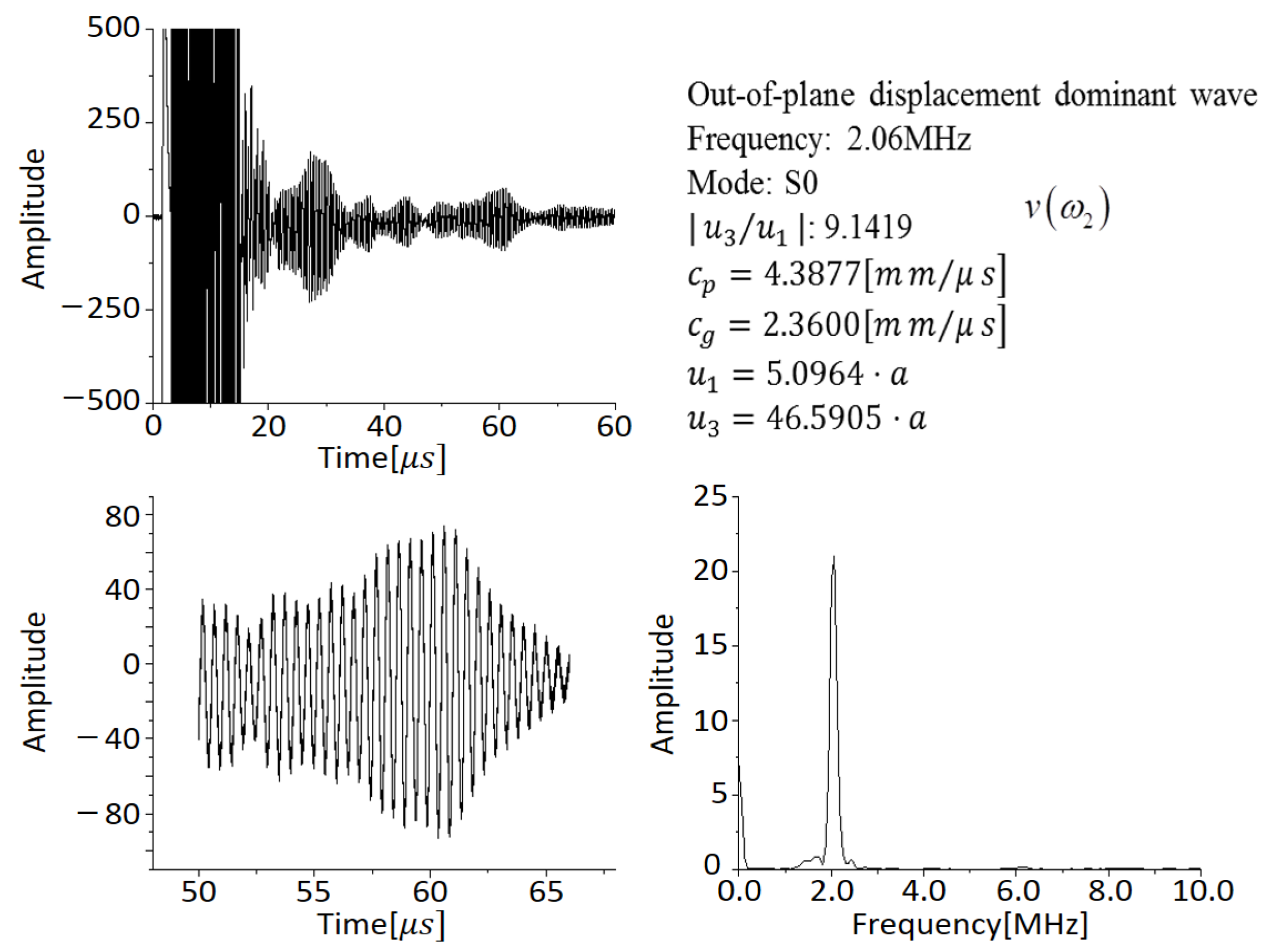
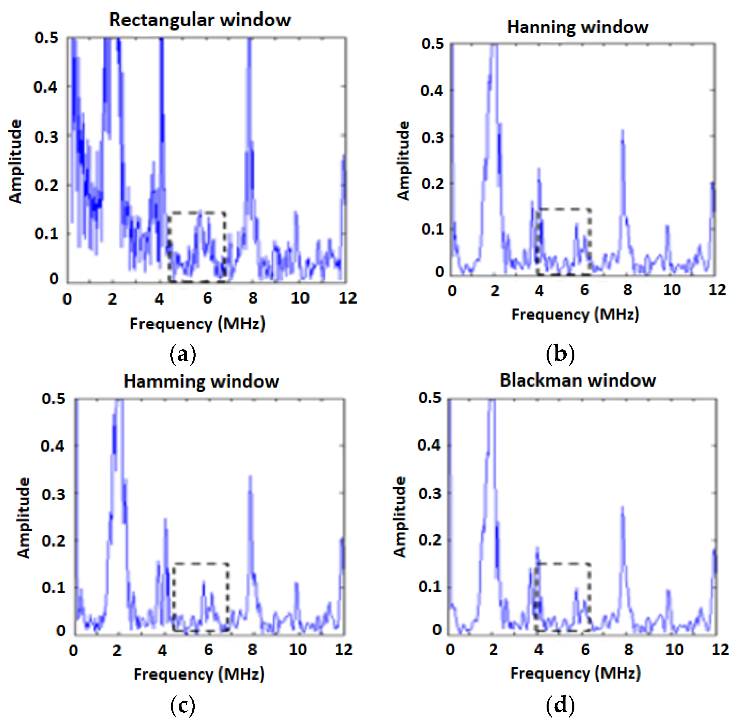
3.2. Standard for Guided Wave Mixing Signal Detection

It is necessary to give standards for guided wave mixing signal detection, and to determine whether a signal is a mixing signal. The frequency of the two primary waves and mixing wave is set by Equations (15) and (18). Table 3 shows the signal data used for analysis to determine standards for detecting a mixing signal. Primary waves are generated individually using No. 1 and 3 in Table 3. Primary waves are generated together using No. 2 in the table. These three sets of data are sufficient for analysis. No. 4 is provided for when the sum of Nos. 1 and 3 is removed from No. 2 for signal processing.
A guided wave mixing single is detected when the following standards are met: Data types No. 2 and 4 have a mixing frequency component (5.77 MHz) in the frequency domain.
The mixing frequency component of No. 2 has much greater amplitude than the other data types in the frequency domain.

4. Results

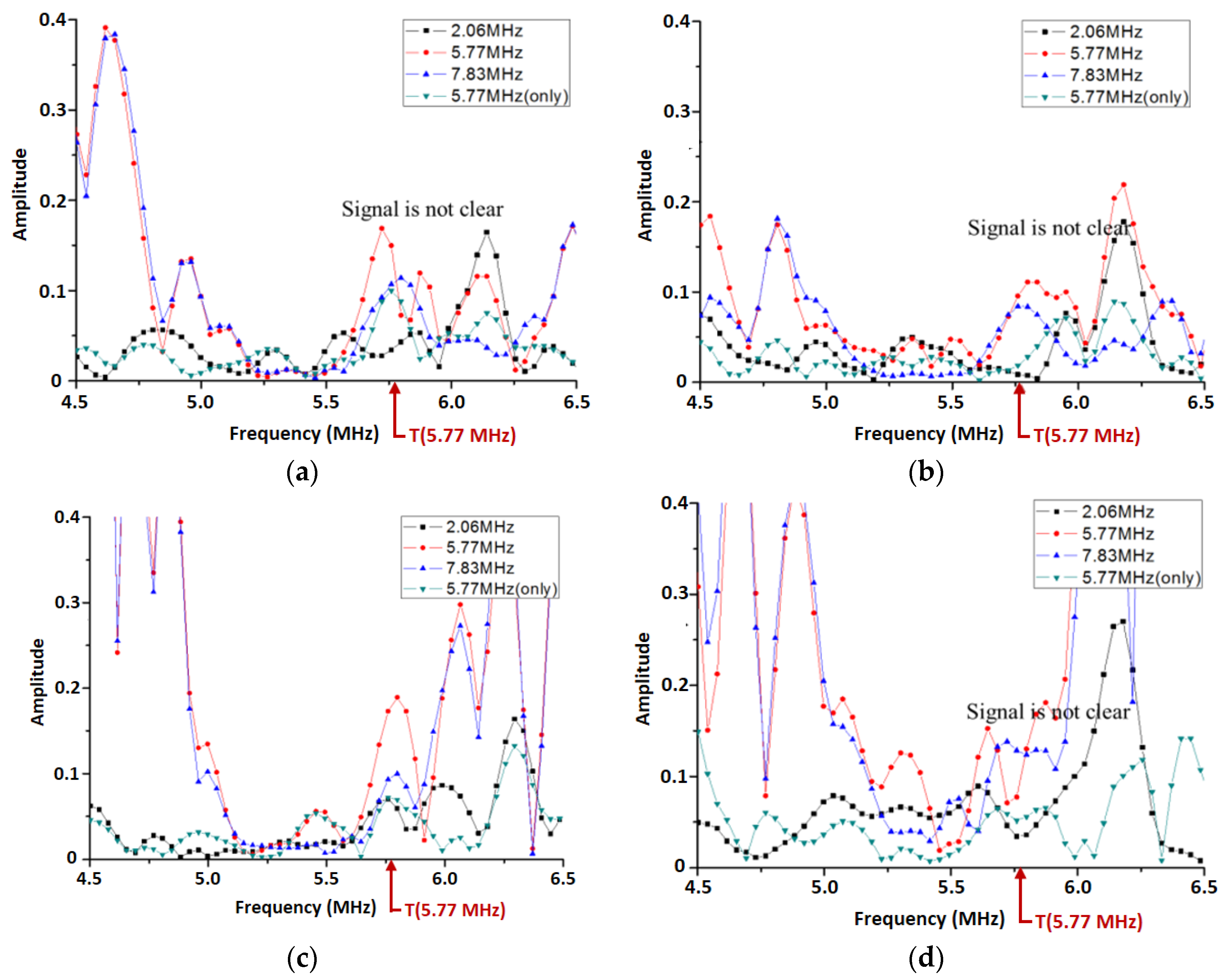
4.1. Experimental Result of Guided Wave Mixing Signal Generation

A mixing signal appears at S1 mode, and the forward direction in the theoretical analysis, but not in the experiment. This result could be interpreted based on the phase velocity. The wedge angle can be determined from the phase velocity. For S1 and A1 modes, the phase velocities of the mixing wave components at 5.77 MHz are ( 4.7282 and 3.3465 )   mm / μ s , respectively. The two primary wave phase velocities are ( 5.8072 and 4.3877 )   mm / μ s , respectively. The S1 mode mixing signal phase velocity is more akin to the primary wave phase velocities than that of the A1 mode. This means that the wedge angle is very similar. In other words, the sensor and wedge receive both the mixing signal and primary waves in the mixing generation experiment with S1 mode. Its situation interrupts frequency analysis. In contrast, the sensor and wedge receive only the mixing signal relatively in the mixing generation experiment with A1 mode, compared to that with S1 mode. Therefore, A1 mode is better for detecting a mixing wave. In mixing signal generation with A1 mode and the forward direction, only a mixing component is detected.

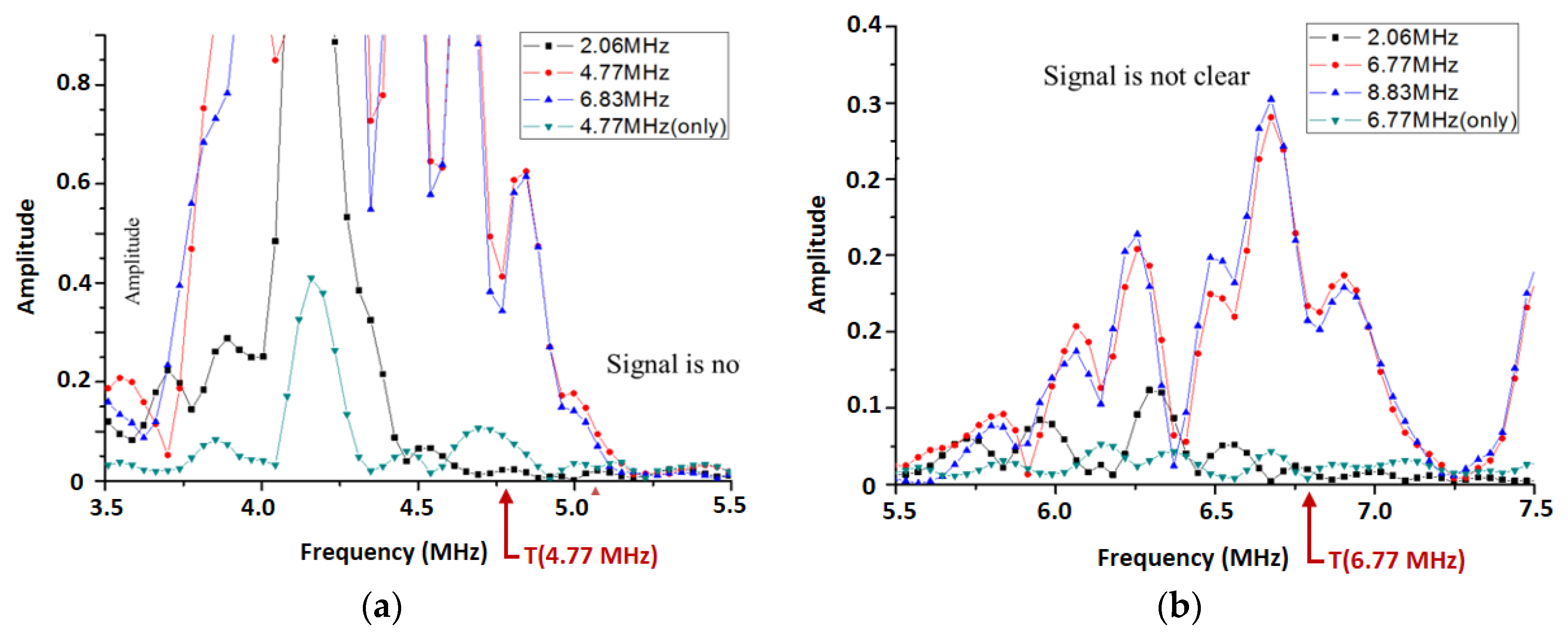
4.2. Comparison of Guided Wave Mixing Technique and Phase Matching Mode Experimental Setup and Results

To examine the feasibility of the guided wave mixing technique, the results were compared with phase matching mode results for the same specimen. Figure 14a,b show the experimental diagrams for the phase matching mode technique and guided wave mixing technique.   b means the mixing wave propagation distance (the scan range). As the distance is changed, nonlinearity is also measured ( a = 125   mm ,   b = 50   mm ,   55   mm , ,   85   mm ). Table 4 and Table 5 give information about the experimental setup. Even though the two experimental setups are based on different mode and frequency, it is worthwhile to compare the results, because the data type that is used for study is not absolute data, but relative data (nonlinearity variation). Through nonlinearity variation, sensitivity information is estimated.
Figure 15 shows the nonlinearity variation as the receiver distance ( b ) is increased. Both graphs show the nonlinearity increment. The same tendencies are observed for the different techniques. To compare the degree of variation and sensitivity, a graph with the same vertical axis range of the two graphs is inserted in Figure 15a. The results for the guided wave mixing technique represent a big nonlinearity variation difference. This means that the technique is more appropriate for evaluating nonlinearity variation than the phase matching mode technique. The reasons for the good nonlinear sensitivity are as follows:
A mixing signal is not generated directly from the equipment, but is instead newly generated and mixed in the specimen by two primary waves. Therefore, it has less influence from the system. This means the mixing signal contains reduced system nonlinearity.
In the case of the difference frequency mixing component, the system nonlinearity commonly included in the primary waves is canceled out, so the system nonlinearity is reduced.

5. Conclusions

The main purpose of this study is the theoretical and experimental verification of a guided wave mixing technique. The biggest advantage of the mixing technique is the reduction of system nonlinearity. Because the system nonlinearity is not what a user wants, it interrupts the evaluation. We can expect clear nonlinearity variation if the measured nonlinearity contains less system nonlinearity. A part of bulk wave mixing theory was applied for simple or assumed guided wave signals. In order to simplify the guided wave mixing theory study, wave structure was considered. In-plane and out-of-plane dominant displacements for each guided wave were considered as longitudinal and transverse waves in a bulk wave.
It was theoretically and experimentally verified that a certain frequency ratio must be considered for mixing. The guided wave mixing result showed the same tendency as the phase matching mode result, but the guided wave mixing technique had better sensitivity for nonlinear variation, because it has less system nonlinearity. Because of the experimental difficulty, the experimental result contains a large error, so repeated and accurate experiments are necessary. Moreover, nonlinearity variation was only evaluated according to distance. For field applications, experiments with micro-damage, such as that from corrosion, are essential. The significant results in this study are as follows:
In this study, guided wave mixing equations and terms such as frequency ratio and mode are derived, and calculated successfully.
The experimental results and the theoretical expectation matched well. The mixing signal only detected the calculated frequency ratio condition.
Comparison of the results between the conventional technique and guided wave mixing technique indicates that the guided wave mixing technique has less system nonlinearity and more sensitive nonlinear variation.
The final result of this study is that the guided wave mixing technique is the proper method for nonlinear evaluation, compared with the conventional technique, because less system nonlinearity is included.
The nonlinear ultrasonic technique used in this study is used by many researchers as an innovative method that can detect micro-defects, but it was used without considering the nonlinearity of the equipment. Analyzing only the nonlinearity of the material without considering the nonlinearity of the system cannot guarantee the reliability of the results. The guided ultrasonic mixing technique that can reduce system nonlinearity is expected to decrease experimental errors and analyze micro-defects in materials more quantitatively.

Author Contributions

J.P. and J.C. designed and performed the experiments. J.L. and J.C. conceived the original idea. J.P. developed the theory, and performed the computations with support from J.L. and J.C. verified the analytical methods. J.C. wrote the draft study, J.P. completed the final study, and J.L. made the final review. All authors have read and agreed to the published version of the manuscript.

Funding

This work was supported by the National Research Foundation of Korea(NRF) grant funded by the Korea government(MSIT) (No. 2019R1A5A808320112).

Conflicts of Interest

The authors declare no conflict of interest.

References

  1. Pruell, C.; Kim, J.-Y.; Qu, J.; Jacobs, L.J. Evaluation of plasticity driven material damage using Lamb waves. Appl. Phys. Lett. 2007, 91, 231911. [Google Scholar] [CrossRef]
  2. Kim, J.-Y.; Jacobs, L.; Qu, J.; Littles, J.W. Experimental characterization of fatigue damage in a nickel-base superalloy using nonlinear ultrasonic waves. J. Acoust. Soc. Am. 2006, 120, 1266–1273. [Google Scholar] [CrossRef]
  3. Cantrell, J.H.; Yost, W. Nonlinear ultrasonic characterization of fatigue microstructures. Int. J. Fatigue 2001, 23, 487–490. [Google Scholar] [CrossRef]
  4. Liu, M.; Tang, G.; Jacobs, L.; Qu, J.; Thompson, D.O.; Chimenti, D.E. Measuring acoustic nonlinearity by collinear mixing waves. AIP Conf. Proc. 2011, 1335, 322. [Google Scholar] [CrossRef]
  5. Achenbach, J.D.; Wang, Y. Far-field resonant third harmonic surface wave on a half-space of incompressible material of cubic nonlinearity. J. Mech. Phys. Solids 2018, 120, 5–15. [Google Scholar] [CrossRef]
  6. Jeong, H.; Choi, S. Ultrasonic measurement of the nonlinear parameter using third harmonic waves—1. Theory. J. Korean Soc. Nondestruct. Test. 2021, 41, 50–58. [Google Scholar] [CrossRef]
  7. Croxford, A.J.; Wilcox, P.D.; Drinkwater, B.W.; Nagy, P.B. The use of non-collinear mixing for nonlinear ultrasonic detection of plasticity and fatigue. J. Acoust. Soc. Am. 2009, 126, EL117–EL122. [Google Scholar] [CrossRef] [PubMed] [Green Version]
  8. Jones, G.L.; Kobett, D.R. Interaction of Elastic Waves in an Isotropic Solid. J. Acoust. Soc. Am. 1963, 35, 5–10. [Google Scholar] [CrossRef]
  9. Taylor, L.H.; Rollins, J.F.R. Ultrasonic Study of Three-Phonon Interactions. I. Theory. Phys. Rev. 1964, 136, A591–A596. [Google Scholar] [CrossRef]
  10. Li, F.; Zhao, Y.; Cao, P.; Hu, N. Mixing of ultrasonic Lamb waves in thin plates with quadratic nonlinearity. Ultrasonics 2018, 87, 33–43. [Google Scholar] [CrossRef]
  11. Jingpin, J.; Xiangji, M.; Cunfu, H.; Bin, W. Nonlinear Lamb wave-mixing technique for micro-crack detection in plates. NDT E Int. 2017, 85, 63–71. [Google Scholar] [CrossRef]
  12. Qureshi, K.K.; Wang, S.H.; Wai, P.; Tam, H.Y.; Lu, C.; Sugimoto, N. Width-tunable pulse generation using four-wave mixing in bismuth based highly nonlinear fiber. Opt. Commun. 2007, 275, 223–229. [Google Scholar] [CrossRef]
  13. Lin, S.; Wang, Z.; Li, J.; Chen, S.; Rao, Y.; Peng, G.; Gomes, A.S.L. Nonlinear dynamics of four-wave mixing, cascaded stimulated Raman scattering and self Q-switching in a common-cavity ytterbium/Raman random fiber lase. Opt. Laser Technol. 2021, 134, 106613. [Google Scholar] [CrossRef]
  14. Zhu, W.; Deng, M.; Xiang, Y.; Xuan, F.-Z.; Liu, C.; Wang, Y.-N. Modeling of ultrasonic nonlinearities for dislocation evolution in plastically deformed materials: Simulation and experimental validation. Ultrasonics 2016, 68, 134–141. [Google Scholar] [CrossRef]
  15. Liu, X.; Bo, L.; Liu, Y.; Zhao, Y.; Zhang, J.; Hu, N.; Fu, S.; Deng, M. Detection of micro-cracks using nonlinear lamb waves based on the Duffing-Holmes system. J. Sound Vib. 2017, 405, 175–186. [Google Scholar] [CrossRef]
  16. Li, W.; Hu, S.; Deng, M. Combination of Phase Matching and Phase-Reversal Approaches for Thermal Damage Assessment by Second Harmonic Lamb Waves. Materials 2018, 11, 1961. [Google Scholar] [CrossRef] [Green Version]
  17. Guan, R.; Lu, Y.; Wang, K.; Su, Z. Fatigue crack detection in pipes with multiple mode nonlinear guided waves. Struct. Health Monit. 2018, 18, 180–192. [Google Scholar] [CrossRef]
  18. Park, J.; Lee, J.; Min, J.; Cho, Y. Defects Inspection in Wires by Nonlinear Ultrasonic Guided Wave Generated by Electro-magnetic Sensors. Appl. Sci. 2020, 10, 4479. [Google Scholar] [CrossRef]
  19. Metya, A.K.; Tarafder, S.; Balasubramaniam, K. Nonlinear Lamb wave mixing for assessing localized deformation during creep. NDT E Int. 2018, 98, 89–94. [Google Scholar] [CrossRef] [Green Version]
  20. Yeung, C.; Tai, N.G. Nonlinear guided wave mixing in pipes for detection of material nonlinearity. J. Sound Vib. 2020, 485, 115541. [Google Scholar] [CrossRef]
  21. Sun, M.; Qu, J. Analytical and numerical investigations of one-way mixing of Lamb waves in a thin plate. Ultrasonics 2020, 108, 106180. [Google Scholar] [CrossRef]
  22. Blanloeuil, P.; Rose, L.; Veidt, M.; Wang, C. Nonlinear mixing of non-collinear guided waves at a contact interface. Ultrasonics 2021, 110, 106222. [Google Scholar] [CrossRef] [PubMed]
  23. Ishii, Y.; Hiraoka, K.; Adachi, T. Finite-element analysis of non-collinear mixing of two lowest-order antisymmetric Rayleigh–Lamb waves. J. Acoust. Soc. Am. 2018, 144, 53–68. [Google Scholar] [CrossRef] [PubMed]
  24. Choi, H.; Lee, J.; Cho, Y. Experimental Study on Corrosion Detection of Aluminum alloy using Lamb wave Mixing Technique. Trans. Korean Soc. Mech. Eng. 2016, 40, 919–925. [Google Scholar] [CrossRef]
  25. Lee, J.; Choi, J.; Choi, H.; Cho, Y. Evaluation of Corrosion of a Material Using Guided Ultrasonic Mixing Technique. Trans. Korean Soc. Mech. Eng. A 2017, 41, 1203–1208. [Google Scholar] [CrossRef]
  26. Cho, H.J.; Hasanian, M.; Shana, S.; Lissenden, C.J. Nonlinear guided wave technique for localized damage detection in plates with surface-bonded sensors to receive Lamb waves generated by shear-horizontal wave mixing. NDT E Int. 2019, 102, 35–46. [Google Scholar] [CrossRef]
  27. Shan, S.; Hasanian, M.; Cho, H.; Lissenden, C.J.; Cheng, L. New nonlinear ultrasonic method for material characterization: Codirectional shear horizontal guided wave mixing in plate. Ultrasonics 2019, 96, 64–74. [Google Scholar] [CrossRef]
  28. Li, W.; Xu, Y.; Hu, N.; Deng, M. Impact damage detection in composites using a guided wave mixing technique. Meas. Sci. Technol. 2019, 31, 014001. [Google Scholar] [CrossRef]
  29. Ju, T.; Achenbach, J.D.; Jacobs, L.J.; Qu, J. Nondestructive evaluation of thermal aging of adhesive joints by using a nonlinear wave mixing technique. NDT E Int. 2019, 103, 62–67. [Google Scholar] [CrossRef]
  30. Viktorov, I.A. Rayleigh and Lamb Waves: Physical Theory and Applications; Plenum Press: New York, NY, USA, 1967. [Google Scholar]
  31. Rose, J.L.; Nagy, P.B. Ultrasonic Waves in Solid Media; Cambridge University Press: Cambridge, MA, USA, 2014. [Google Scholar]
  32. Norris, A.N. Finite Amplitude Waves in Solids: Nonlinear Acoustics; Academic Press: San Diego, CA, USA, 1998. [Google Scholar]
  33. Korneev, V.A.; Nihei, K.T.; Myer, L.R. Nonlinear Interaction of Elastic Waves in Solids; University of California: Berkeley, CA, USA, 1988. [Google Scholar]
  34. Krasilnikov, V.; Zarembo, L. Nonlinear Interaction of Elastic Waves in Solids. IEEE Trans. Sonics Ultrason. 1967, 14, 12–17. [Google Scholar] [CrossRef]
  35. Deng, M. Cumulative second-harmonic generation of Lamb-mode propagation in a solid plate. J. Appl. Phys. 1999, 85, 3051–3058. [Google Scholar] [CrossRef]
  36. Li, W.; Cho, Y.; Achenbach, J.D. Detection of thermal fatigue in composites by second harmonic Lamb waves. Smart Mater. Struct. 2012, 21, 085019. [Google Scholar] [CrossRef]
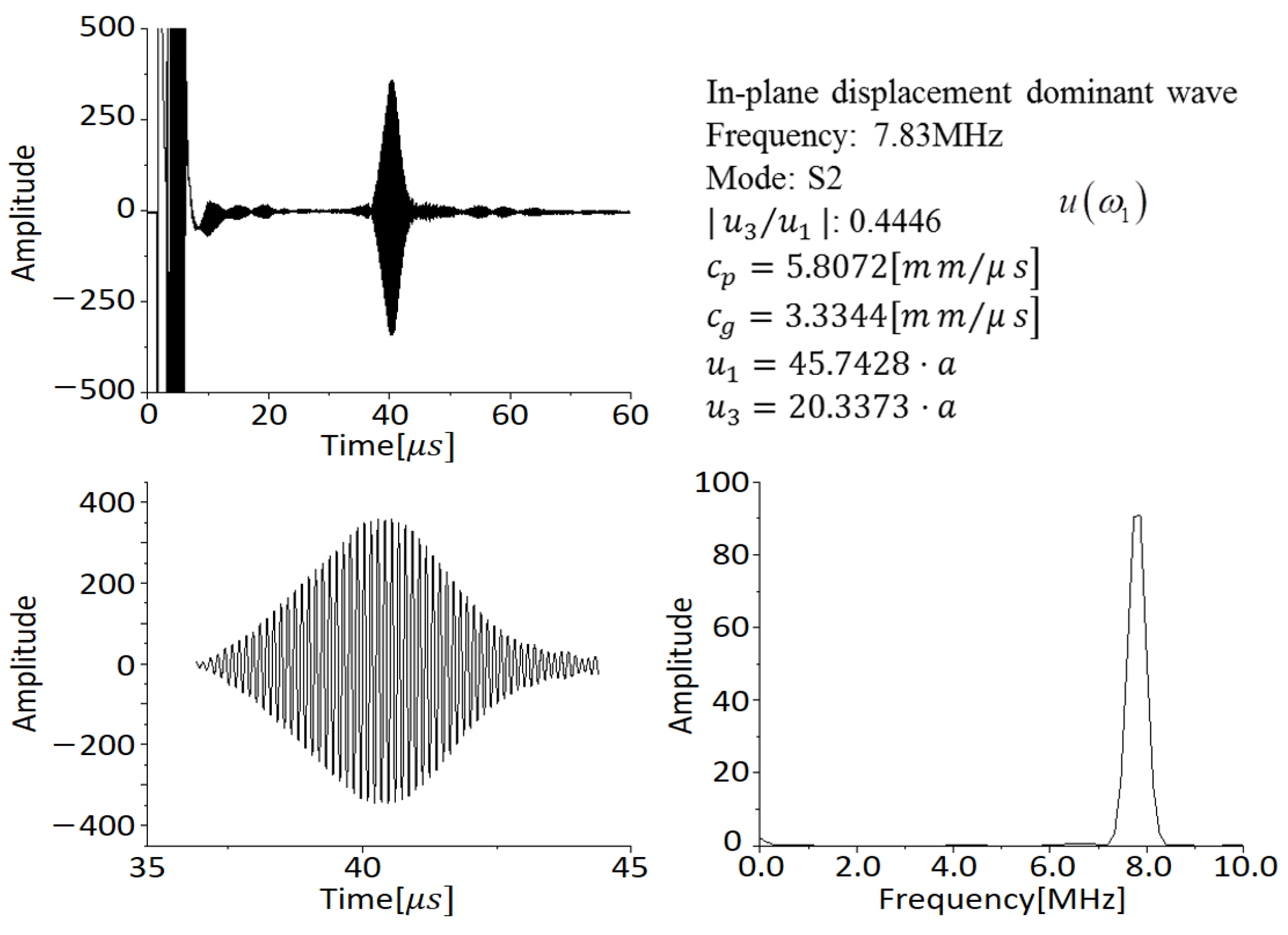
Figure 1. In-plane ( u 1 ) and out-of-plane ( u 3 ) displacement coordinate diagram.
Applsci 11 06569 g001
Figure 2. Diagram of the guided wave mixing concept on a plate.
Applsci 11 06569 g002
Figure 4. Dispersion curve (Al 1050). (a) Phase velocity with double symmetric mode; (b) Group velocity with double symmetric mode.
Applsci 11 06569 g004
Figure 5. Dispersion curve showing primary and mixing waves: (a) Phase velocity; (b) Group velocity.
Applsci 11 06569 g005
Figure 6. Basic experimental sensor arrangement.
Applsci 11 06569 g006
Figure 7. Experimental setup for material evaluation by guided wave mixing.
Applsci 11 06569 g007
Figure 8. Experimental setup with S1, A1 modes and two directions: (a) Forward direction S1, A1 modes; (b) Inverse direction S1, A1 modes (a = 100 mm and |b| = 20 mm).
Applsci 11 06569 g008
Figure 9. Wave velocity and frequency analysis for 7.83 MHz (S2 mode).
Applsci 11 06569 g009
Figure 10. Wave velocity and frequency analysis for 2.06 MHz (S0 mode).
Applsci 11 06569 g010
Figure 11. FFT results: (a) Rectangular window; (b) Hanning window; (c) Hanmming window; (d) Blackman window.
Applsci 11 06569 g011
Figure 12. Frequency domain analysis results: (a) S1 mode, forward direction; (b) S1 mode, inverse direction; (c) A1 mode, forward direction; (d) A1 mode, inverse direction.
Applsci 11 06569 g012
Figure 13. Frequency analysis results: (a) A1 mode, forward direction u ( 6.83   MHz ) + v ( 2.06   MHz ) v ( 4.77   MHz ) ; (b) A1 mode, inverse direction u(8.83 MHz) + v(2.06 MHz) → v(6.77 MHz).
Applsci 11 06569 g013
Figure 14. Experimental Setup: (a) Phase matching mode; (b) Guided wave mixing technique.
Applsci 11 06569 g014
Figure 15. Nonlinearity variation depending on the receiver position with the same vertical range: (a) Phase matching mode; (b) Guided wave mixing.
Applsci 11 06569 g015
Table 1. Primary wave information.
Frequency7.83 MHz2.06 MHz
ModeS2S0
| u 3 / u 1 | , Dispersion ratio0.44469.1419
c p [ mm / μ s ] , Phase velocity5.80724.3877
c g [ mm / μ s ] , Group Velocity3.33442.3600
u 1 , In-plane displacement45.7428 a5.0964 b
u 3 , Out-plane displacement20.3373 a46.5905 b
Table 2. Information for the two types of modes at 5.77 MHz.
Frequency5.77 MHz5.77 MHz
ModeS1A1
| u 3 / u 1 | , Dispersion ratio2.82792.3929
c p [ mm / μ s ] , Phase velocity4.72823.4265
c g [ mm / μ s ] , Group Velocity2.34902.4114
u 1 , In-plane displacement61.7937 c295.5737 c
u 3 , Out-plane displacement174.7443 d707.2642 d
Table 3. Data used for analysis, u ( 7.83   MHz ) + v ( 2.06   MHz ) v ( 5.77   MHz ) .
No.Type of DataExplanationRemarks
12.06 MHzOnly 2.06 MHz is generatedExperimental result
25.77 MHzBoth (2.06 and 7.38) MHz are generated at the same timeExperimental result
37.83 MHzOnly 7.83 MHz is generatedExperimental result
45.77 MHzNo.2 (−) (No.1 + No.3)Signal processing result
Table 4. Experimental conditions for phase matching mode technique.
FrequencyTypeFrequencyWedge Angle
Pulser3.5 MHz ω 1 = 3.41   MHz25°
Receiver7.5 MHz ω 2 = 6.82   MHz25°
Table 5. Experimental conditions for guided wave mixing technique.
FrequencyTypeFrequencyWedge Angle
Pulser10 MHz
2.25 MHz
ω 1 = 7.83   MHz
ω 2 = 2.06   MHz
25°
37°
Receiver7.5 MHz ω 1 ω 2 = 5.77   MHz52°
Publisher’s Note: MDPI stays neutral with regard to jurisdictional claims in published maps and institutional affiliations.

