Push/Pull Parts Production Policy Optimization in the ATO Environment

Abstract

Within the Assembly to Order (ATO) production strategy, the common approach is to produce the parts to assemble with a Push-Make to Stock policy.In recent decades, the effects of the modern Just in Time (JIT) moved to a Pull-Make to Order policy. Assembled parts characterized by wide variety and huge storage space utilization are critical, and a proper Push/Pull production policy definition is required. An appropriate balance of storage space utilization and setup times leads to the optimization of the production policy. The aim of this paper is to define a bi-objective mathematical optimization model to assign the most suitable production policy to the parts within the production mix in an ATO industrial context. A numerical simulation and an operative case study showcases the model application, proving the industrial relevance of this research.

1. Introduction

Offering differentiated products is essential for many manufacturing companies. To reach high levels of efficiency and throughput, they developed product platforms, implementing product standardization and modularization. These elements offered the possibility to implement the Assembly to Order (ATO) paradigm, permitting low time to market and high level of product personalization [1,2,3]. In the ATO context, assembly is performed with a Just in Time (JIT) approach, while the parts manufacturing and procurement lead times are masked by the stock. The ATO production strategy typically uses a Pull-Make to Order in the assembly phase and a Push-Make to Stock strategy before the assembly phase according to forecasts or storage reorder points [4]. The pure Make to Stock (MTS) production strategy aims to preventing stock-out risks, and its main advantage is the reactivity to fulfil the demands. The performance criteria in MTS production planning are usually cost-based [5]. In fact, MTS policy can have a negative impact on many operative aspects: the inventory costs, the space utilization, the production capacity utilization, etc.

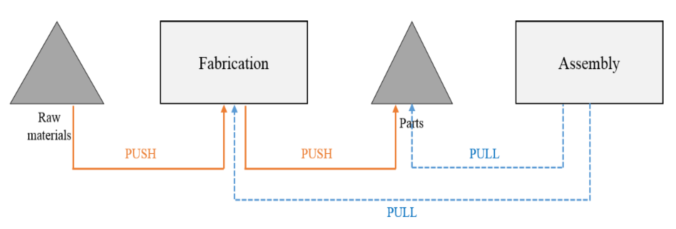
As consequence, many companies tried to adopt some strategies to mitigate this problem. A possible strategy is to apply for the parts with these attributes an MTO-Pull production policy instead of an MTS-Push policy. The result will be a hybrid Push/Pull policy applied to the internally manufactured parts used in assembly (Figure 1). As demonstrated by many studies in the field [6,7,8], in recent years industrial companies are moving toward the implementation of hybrid MTO/MTS production strategies. Technological developments in manufacturing systems increasingly allow companies to manufacture different products on the same production facility with hybrid approaches [9]. For example, low-valued, standardized products will often be made to stock, allowing demand to be satisfied instantly. For high valued products with irregular demand, stocking can be expensive or even impossible, and these are typically produced to order [10].

A proper combination of (Make To Order/Make To Stock) MTO/MTS policies can exploit the advantages of both lower inventory and short delivery time [11]. It needs to be optimized for each part as function of its attributes and in accordance with the production system constraints.

From a practical point of view, there are many implications. The proposed approach can be applied to different manufacturing technologies: cutting, bending, welding, painting, machining, etc. Secondly, different parts typologies can be interested in a Pull production policy as an effect of their wide variety, huge storage space utilization, and relevant cost. For example, the product frames, the product structure, the switchboards, the electrical engines, the pumps, the plastic parts, etc.

The aim of this paper is to explore the chance of using flexibility in production to cope with the wide product variety by applying a hybrid Push/Pull production for internally produced parts to define the best policy to apply for each of them.

The novelty of the paper is represented by the proposed bi-objective mathematical optimization model to properly set for each part the Push or Pull policy to minimize setup time and the inventory used space by using a multicriteria approach. A key element of the research is the adoption of operative objective functions instead of a general cost-based approach. In fact, productive and logistic attribute of the parts are considered because they strongly impact on the process. Consequently, the maximum number of units that can be stacked on a Euro Pallet (EPAL) (logistic parameter) and the agility (production parameter) are considered in the proposed optimization model. A further element of interest of this research is the consideration of the concept of agility in the hybrid Push/Pull policy definition, i.e., the ability of the upstream production system to rapidly cope with a variable market demand [12,13].

The practical implications of the research are relevant. In fact, its applicability is wide and related to different industrial contexts. A numerical simulation and a case study of an Italian manufacturer are reported to describe, test, and demonstrate the proposed model and the practical implications of this research.

The remainder of this paper is organized as follows: Section 2 reviews the relevant literature on the topic. In Section 3, the bi-objective optimization model for Push/Pull policy definition in ATO environment is introduced and described, while Section 4 reports the case study and discusses the main results. Finally, Section 5 concludes the paper with final remarks and future opportunities for research.

2. Literature Review

Reduced product life cycles, dynamic market demand, and flexible production cycles are rising as crucial challenges for most industrial companies [2]. In such a context, the assignment of the best production strategy, i.e., Pull-MTO or Push-MTS to each item within the production mix is a strategic issue.

Table 1 represents a schematic representation of some recent and important contributions on hybrid MTS/MTO policy definition with the aim of highlighting the objective, the proposed method, and the reported case study. Even if a wide set of researchers and industrial practitioners investigates hybrid MTS/MTO production systems, so far, a limited number of studies was published in this field [14]. Moreover, the few published papers do not focus on manufacturing within an ATO environment. A relevant contribution on hybrid MTS/MTO was the study proposed by Williams [15], which focused on one-stage systems with stochastic demands and capacity constraints through queuing theory. The main goal of the proposed algorithm was to select the items to be managed with MTS production strategy. Furthermore, in this field, other relevant studies were proposed with different goals. According to Table 1, the main optimization objectives are related to:

• the determination of the decoupling point between MTO and MTS, i.e., by analyzing the flow of the different production stages, the goal is to find separation point between the upstream MTS strategy and the downstream MTO strategy where the generic products are post manufactured and customized [8,10,11,16,17,18,19].
• Optimization of the production planning & scheduling phases by applying a suitable MTS/MTO strategy [5,14,20,21,22,23,24,25,26,27].
• Order acceptance and capacity requirement, including production resource constraints, material supplies, and dynamic changes in the market context [4,6,20,23]
• Inventory management according to the MTS policy [14,16,19,22,28,29,30,31,32,33].

The presence of different objectives explored by researchers in the MTO/MTS policy definition stresses the complexity and relevance of the problem.

On the other hand, just a few authors propose multiobjective models, addressing multiple goals simultaneously. As an example, Wang et al. [22] propose a hybrid algorithm for order acceptance and scheduling problem in MTO/MTS industries. Almehdawe and Jewke [24] introduce a batch ordering policy to permit economies of scale. Zhang et al. [29] propose an optimization model to find the optimal intermediate buffer size considering earliness/tardiness penalty, inventory cost, production penalty, inventory matching, and order cancellation penalty.

Moreover, as by the Table 1, different approaches were proposed, e.g., mathematical single- or multiobjective optimization models, heuristic algorithms, decision process models based on Markov chains, or on decisional frameworks, simulation models, etc.

The use of industrial case studies is not often present and well-described in the existing research. In fact, the use of numerical analysis is widespread to test the proposed methodologies. The case studies reported by some authors belong to different industrial sectors, demonstrating the cross-interest of this research topic.

The literature review highlights that authors focus on defining single-objective models, even if in the hybrid Push/Pull policy definition problem a set of objectives exists, which need to be managed and best balanced. On the other hand, the few contributions proposing multiobjective formulations do not propose a robust multicriteria approach. According to this background, this paper aims at proposing a bi-objective mathematical optimization model supporting the hybrid Push/Pull policy definition to jointly minimize the setup time and the storage used space, getting the final Pareto frontier of the optimal solutions [31]. As demonstrated by Lu et al. [31], this approach shows relevant improvements towards the classic desirability function methods. In addition, a relevant metric is considered in this research to guide the selection of the parts to manage with a Pull approach. Such a metric is represented by the agility parameter, which is a combination of production system speed and flexibility.

Table 1. Hybrid PUSH/PULL literature analysis.

Reference		Objective				Method					Case Study
		Optimization of the MTS/MTO decoupling point	Optimization of production, planning and scheduling	Optimization of order acceptance	Optimization of Inventory managemen	Framework	Algorithm	Simulation/ Comparison model	Mixed Integer Programming	Markov Decision Process Model	Numerical analysis	Mechanical Industry	Domestic appliance Industry	Wood Indusrty	Chemical Industry	Ceramic Tile Industry	Steel Industry	Food Industry	Foundry Industry	Bar turning Industry	Electronic Industry
[4]	Lu and Chen, 2018			X				X
[26]	Kim and Min, 2018				X					X	X
[20]	Wang et al., 2018		X	X		X	X		X		X
[5]	Beemsterboer et al., 2017		X					X			X
[16]	Jia et al, 2017	X			X			X			X
[21]	Wilson, 2017		X							X					X
[22]	Almehdawe and Jewkes, 2013		X		X		X		X		X
[14]	Rafiei et al., 2013		X		X		X
[24]	Cheng et al., 2012		X				X				X
[23]	Rafiei and Rabbani, 2012		X	X				X						X
[6]	Kalantari et al., 2011			X			X		X		X
[27]	Zhang et al., 2011		X		X		X		X								X
[8]	Hemmati and Rabbani, 2010	X				X							X
[25]	Lyonnet et al., 2010		X					X												X
[7]	Eivazy et al., 2009		X					X													X
[28]	Persona et al., 2007				X			X				X
[18]	Soman, 2005	X						X										X
[19]	Corry, P., Kozan, E, 2004	X			X		X												X
[10]	Van Donk, 2001	X				X												X
[30]	Azzamouri et al., 2021	X			X		X
[31]	Varlas et al., 2021	X			X
[32]	Kumar et al., 2019	X			X	X						X									X
[33]	Ciechanska and Szwed, 2020				X			X				X

Table 1. Hybrid PUSH/PULL literature analysis.

Reference		Objective				Method					Case Study
		Optimization of the MTS/MTO decoupling point	Optimization of production, planning and scheduling	Optimization of order acceptance	Optimization of Inventory managemen	Framework	Algorithm	Simulation/ Comparison model	Mixed Integer Programming	Markov Decision Process Model	Numerical analysis	Mechanical Industry	Domestic appliance Industry	Wood Indusrty	Chemical Industry	Ceramic Tile Industry	Steel Industry	Food Industry	Foundry Industry	Bar turning Industry	Electronic Industry
[4]	Lu and Chen, 2018			X				X
[26]	Kim and Min, 2018				X					X	X
[20]	Wang et al., 2018		X	X		X	X		X		X
[5]	Beemsterboer et al., 2017		X					X			X
[16]	Jia et al, 2017	X			X			X			X
[21]	Wilson, 2017		X							X					X
[22]	Almehdawe and Jewkes, 2013		X		X		X		X		X
[14]	Rafiei et al., 2013		X		X		X
[24]	Cheng et al., 2012		X				X				X
[23]	Rafiei and Rabbani, 2012		X	X				X						X
[6]	Kalantari et al., 2011			X			X		X		X
[27]	Zhang et al., 2011		X		X		X		X								X
[8]	Hemmati and Rabbani, 2010	X				X							X
[25]	Lyonnet et al., 2010		X					X												X
[7]	Eivazy et al., 2009		X					X													X
[28]	Persona et al., 2007				X			X				X
[18]	Soman, 2005	X						X										X
[19]	Corry, P., Kozan, E, 2004	X			X		X												X
[10]	Van Donk, 2001	X				X												X
[30]	Azzamouri et al., 2021	X			X		X
[31]	Varlas et al., 2021	X			X
[32]	Kumar et al., 2019	X			X	X						X									X
[33]	Ciechanska and Szwed, 2020				X			X				X

3. Bi-Objective Model for Push/Pull Policy Selection in an ATO Environment

The section shows the full formulation of the proposed bi-objective mathematical model for Push/Pull policy definition in ATO environment.

The proposed optimization approach looks at the problem with an operative perspective. For this reason, the two proposed objective functions consider both production and logistic aspects of the problem: the total setup time and the total space utilization. This is a key attribute of the research, and the union of these two inhomogeneous operative factors is developed according to a bi-objective model based on the Lu et al. (2012) multi-objective Pareto Frontier. The proposed approach considers only the internally produced parts. Consequently, the constrain is related to the available manufacturing technologies where the cycles must be sequential, with no external supplier procurement or production phase. Production scheduling, capacity, and due date are not considered in the model. This assumption is justified by the utilization of the agility concept related to the production throughput, as better explained in the next sections and by the strategic and nonoperative aim of the proposed approach.

The process variability is considered negligible because the basic objective functions that are considered in the research are storage space and setup times which are defined once the item is identified.

3.1. Nomenclature

Indices
$i=$	1:…,I parts
$j=$	1,…,J production processes
$v=$	Production strategy (MTO or MTS)
Part Parameters
$a_i$	agility of part i [pieces/h2]
$EP{Q}_i$	Equivalent Pallet Quantity, number of parts to be stacked on the pallet of part i [pcs/pallet]
$A{1}_i$	upper limit to the dimension of part i [mm]
$A{2}_i$	lower limit to the dimension of part i [mm]
$T_i$	thickness of part i [mm]
$Q_i$	annual required pieces for part i [pcs/year]
$B_i$	Batch dimension according to MTS policy for part i [pcs/batch] equivalent to the Economic Order Quantity (EOQ) according to (Lyonnet et al., 2010)
$O_i$	Number of orders of the part i in a pure pull MTO policy [orders/year]
$E_{i,v}$	number of productive event of part i for production strategy v [productive event/year]
$P{R}_{i,v}$	number of pallet required by applying the production strategy v to manage part i [pallet]
$EP{Q}_i$	Equivalent Pallet Quantity for part i, i.e., n° of storable parts in an EPAL pallet [pcs/pallet]
$EPB{Q}_i$	Equivalent Pallet Base Quantity for part i, i.e., n° of parts storable in the pallet base [pcs/layer]
$EPH{Q}_i$	Equivalent Pallet Height Quantity for part i, i.e., n° of storable levels of $EPB{Q}_i$ [levels/pallet]
$T_{S_{ij}}$	setup time of part i in the process j [hours/productive event]
$T_{C_{ij}}$	production time of part i in the process j [hours/pieces]
$T_{STO{T}_i}$	total setup time of part i [hours/productive event]
$T_{CTO{T}_i}$	Total production time of part i [hours/pieces]

3.2. Determination of the Parts Parameters

Within the model formulation, two main parameters are defined for each part i, i.e., $a_i$ and $EP{Q}_i$, used in the Push/Pull policy optimization procedure. The first one is the agility $a_i$ assessed as follows:

$$a_i=\frac{3600\ast 3600}{T_{STO{T}_i}\ast T_{CTO{T}_i}}\left[\frac{pieces}{hou{r}^2}\right]$$

(1)

where:

$$T_{CTO{T}_i}={{\displaystyle \sum }}_j^{ }{T}_{C_{ij}}\left[s\right]$$

(2)

$$T_{STO{T}_i}={{\displaystyle \sum }}_j^{ }{T}_{S_{ij}}\left[s\right]$$

(3)

According to Barbazza et al. (2017), the used agility metric measures the ability of the production system to accelerate to meet production changes. In particular, the agility increases when the total setup time and the total production time through the production processes j decrease. According to those definitions, the agility parameter expresses the ability of the production system to respond rapidly to change demands in terms of volume and variety. The utilization of this agility formulation permits consideration of potential candidates for an MTO production policy only the parts with the lowest impact on the production capacity and lowest production lead times, justifying the assumptions about the production capacity and planning.

The second proposed metric is the Equivalent Pallet Quantity $EP{Q}_i,$ representing the used volume of the part i as number of parts that can be stacked on a Euro Pallet (EPAL). EPAL is the most used stock keeping unit, with a base of 1200 mm × 800 mm, as in Equation (5). In Figure 1, right side, $EP{Q}_i=12$. $EP{Q}_i$ is calculated as:

$$EP{Q}_i=EPB{Q}_i\ast EPH{Q}_i\left[\frac{pieces}{pallet}\right]$$

(4)

$EPB{Q}_i$ is assessed according to the part shape (U shape, L shape, and I shape for the flat parts), as follows:

$$EPBQi=\{\begin{array}{ll}max\{\begin{array}{c}\left[\frac{1200}{A{2}_i+T_i}\right]\ast \left[\frac{800}{A{1}_i+T_i}\right]\\ \left[\frac{1200}{A{1}_i+T_i}\right]\ast \left[\frac{800}{A{2}_i+T_i}\right]\end{array}& \mathrm{Stacking}“\mathrm{U-shape}”\mathrm{in}\mathrm{pairs}\\ max\{\begin{array}{c}\begin{array}{c}\left[\frac{1200}{A{2}_i+T_i}\right]\ast \left[\frac{800}{A{1}_i}\right]\\ \left[\frac{1200}{A{1}_i}\right]\ast \left[\frac{800}{A{2}_i+T_i}\right]\end{array}\end{array}& \mathrm{Stacking}“\mathrm{L-shape}”\mathrm{in}\mathrm{pairs}\\ \left[\frac{1200}{A{1}_i}\right]\ast \left[\frac{800}{A{2}_i}\right]& \mathrm{Stacking}“\mathrm{I-shape}”\mathrm{in}\mathrm{pairs}\end{array}$$

(5)

3.3. Objective Functions

The two basic objective functions are:

$P_{TOT}$	number of stored EPAL [pallet]
$T{A}_{TOT}$	global setup time [s/year]

These functions depend by the Push/Pull policy assigned to each part i. The first is the total number of EPAL stored in the industrial warehouse, i.e., the inventory objective. The second computes the total setup time over the considered planning period (year), i.e., the production objective. The related trade-off between these two objective functions is clear. The calculation of these two functions is the follow:

$$P_{TOT}={\displaystyle \sum }_i{\displaystyle \sum }_{v}P{R}_{i,v}\left[pallet\right]$$

(6)

where

$$P{R}_{i,v}=\{\begin{array}{c}\frac{B_i/2}{EP{Q}_i}ifv=MTS\\ 0ifv=MTO\end{array}\left[pallet\right]$$

(7)

As by Equation (7), the number of stored EPAL is set to 0 in case of MTO policy application. Otherwise, it is set to the ratio between the average batch dimension, i.e., $B_i/2$, and the equivalent pallet quantity, i.e., $EP{Q}_i$, in case of MTS policy application.

$$T{A}_{TOT}={\displaystyle \sum }_i{\displaystyle \sum }_v(T_{STO{T}_i}\ast E_{i,v})/3600\left[\frac{hours}{year}\right]$$

(8)

where:

$$E_{i,v}=\{\begin{array}{c}{O}_{i}seif=MTO\left[\frac{productiveevents}{year}\right]\\ \frac{Q_i}{B_i}seif=MTS\left[\frac{productiveevents}{year}\right]\end{array}$$

(9)

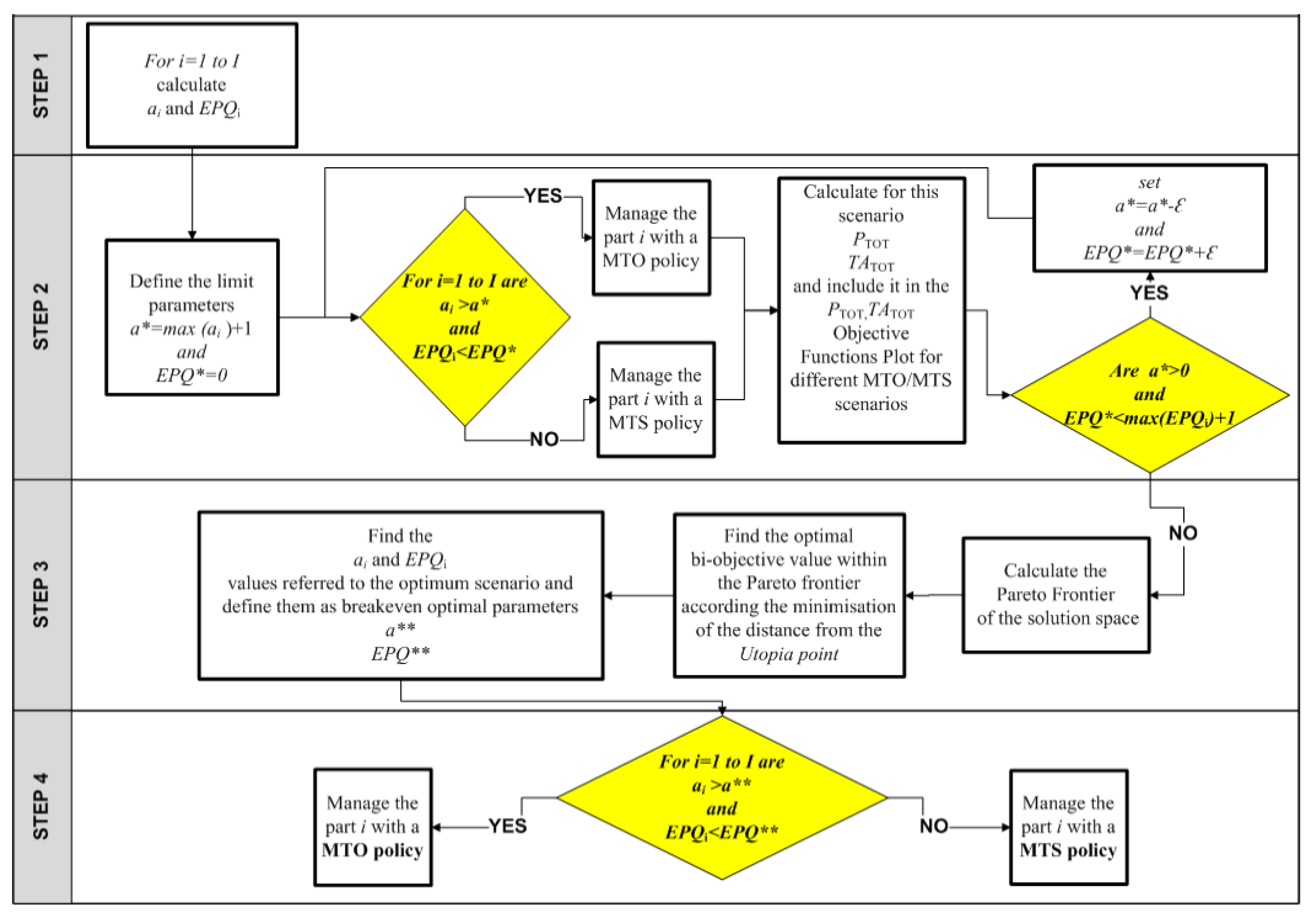
3.4. Algorithm for Push/Pull Policy Selection

The Push/Pull bi-objective procedure aims at assigning to each produced part the best production strategy between a pull and a traditional pure push policy in an ATO environment. The mathematical optimization model aims to minimize storage space and setup times. The procedure is based on four main steps and a schematic flowchart is reported in Figure 2.

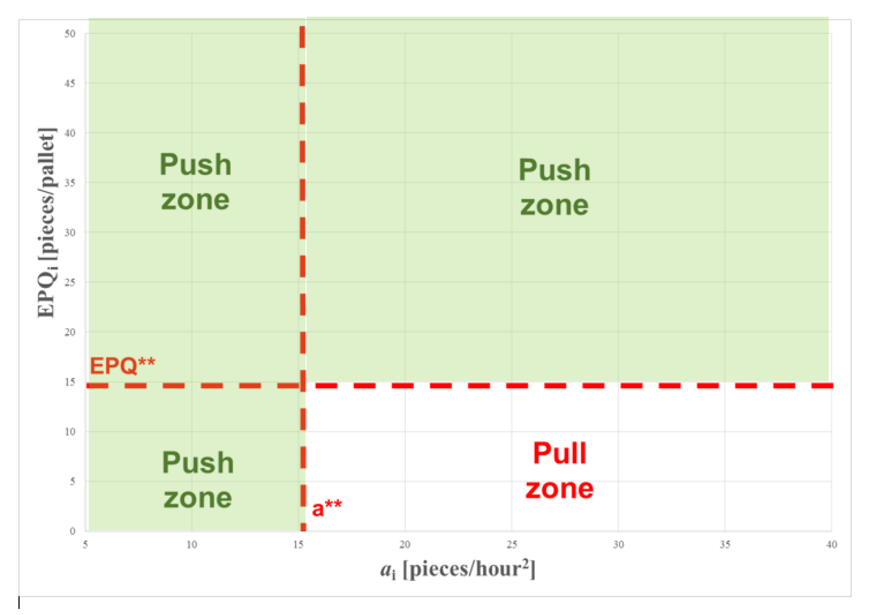
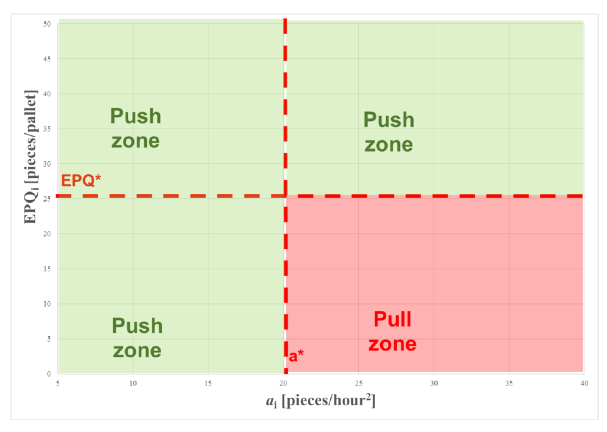
STEP 1. Calculation of the parameters $a_i$ and $EP{Q}_i$ for each part i. In this way, it is possible to graphically define the position of each part. The suitable parts for a Pull policy will be the parts with high values of $a_i$ and low values of $EP{Q}_i$ (as illustrated in Figure 3).

In fact, to produce a part i with a Pull approach, it would be necessary to obtain high values of $a_i$, representing the capacity of the upstream production system to rapidly change the parts to produce and to quickly produce a low number of items instead of an entire production batch. As a consequence, for a part i, low setup time $T_{STO{T}_i}$ Equation (2) and low production time $T_{CTO{T}_i}$ Equation (3) are required within the whole production process (high value of agility $a_i$) to apply a proper Pull policy.

Low values of $EP{Q}_i$, meaning that the most critical parts for a Push policy are those with high dimensions or critical shapes. Consequently, for part i, low values of $EP{Q}_i$ are required to apply a proper Pull policy.

Figure 3 reports the potential Push-Pull zones in the $a_i$ and $EP{Q}_i$ diagram. The optimisation problem lies on the optimal definition of the Pull zone, i.e., the breakeven optimal values of the two parameters a** and EPQ**.

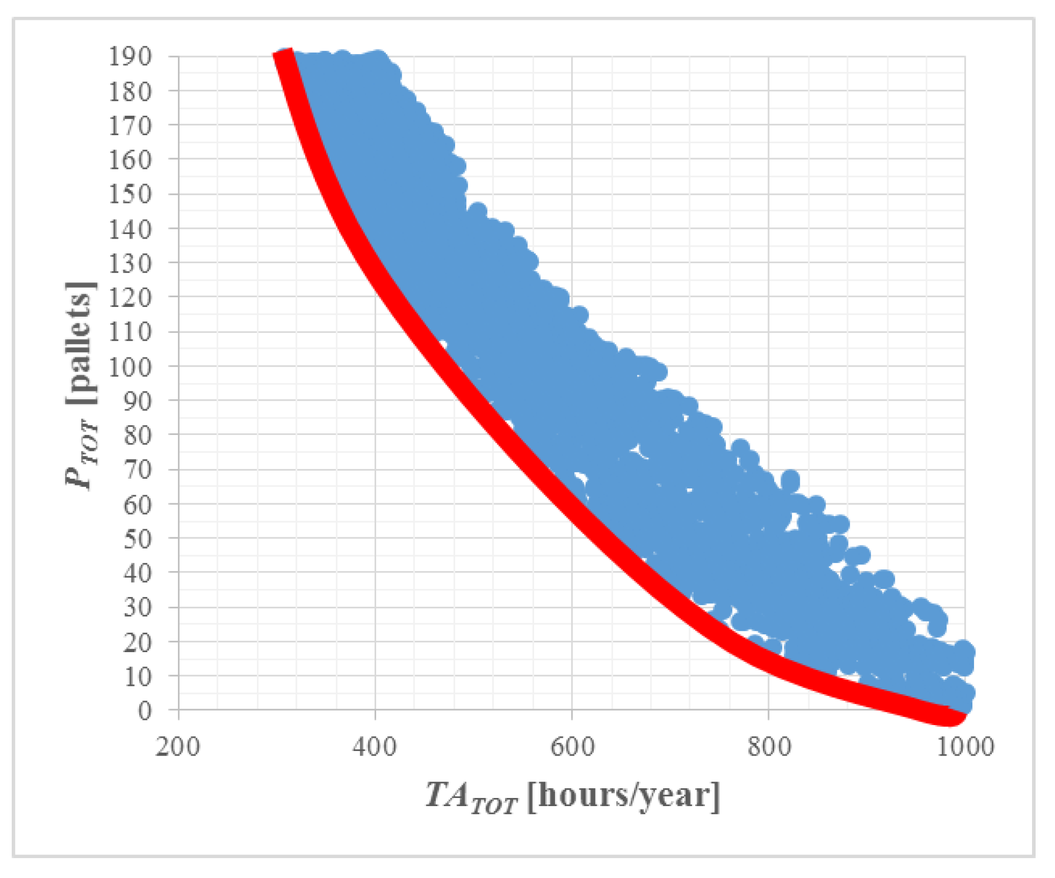
STEP 2. Multiscenario analysis. Considering different values of the two parameters (as illustrated in Figure 3), the values of the two objective functions $P_{TOT}$ and $T{A}_{TOT}$ are assessed.

Main results are in Figure 4 (blue dots) where for each scenario the two objective functions values are plotted.

The procedure adopted to generate and assess the different scenarios is detailed reported in Figure 2 (Step 2). A parameter, i.e., ε, is introduced that can be chosen small enough to generate a representative number of potential scenarios.

STEP 3. Construction of the Pareto frontier of the optimal solutions and breakeven optimal parameters a** and EPQ** definition. According to Lu et al. (2012), starting from the Step 2 results, the dominated and the dominant solutions are found to define the Pareto Frontier.

Figure 4 conceptually reports the Pareto Frontier (red curve) of the different scenarios analyzed in the Step 2 with the points. The set of the points belonging to the Pareto Frontier are defined as $(\overline{T{A}_{TOT}};\overline{P_{TOT})}$.

At this stage, the decision maker needs to select an optimal trade-off solution $(\overline{\overline{T{A}_{TOT}}};\overline{\overline{\overline{P_{TOT})}}}$, among the set of dominant points (Lu et al., 2012). According to Lu et al. (2012) the Utopia point is the point in the solution space corresponding to the optimal values for all criteria. In this case, the Utopia point is the point where the total setup time and the total number of stored EPAL are set to 0:

$$U_{P_{TOT}},U_{T{A}_{TOT}}=\left(0;0\right)$$

(10)

To find the bi-objective optimal point, a method based the minimization of the Euclidean distance between the Utopia point and the points belonging to the Pareto frontier is proposed. It can be defined finding the point $(\overline{\overline{T{A}_{TOT}}};\overline{\overline{\overline{P_{TOT})}}}$ belonging to the Pareto frontier that minimizes:

$$\min \sqrt{\left({\left(\overline{T{A}_{TOT}}-U_{T{A}_{TOT}}\right)}^2+{\left(\overline{P_{TOT}}-U_{P_{TOT}}\right)}^2\right)}$$

(11)

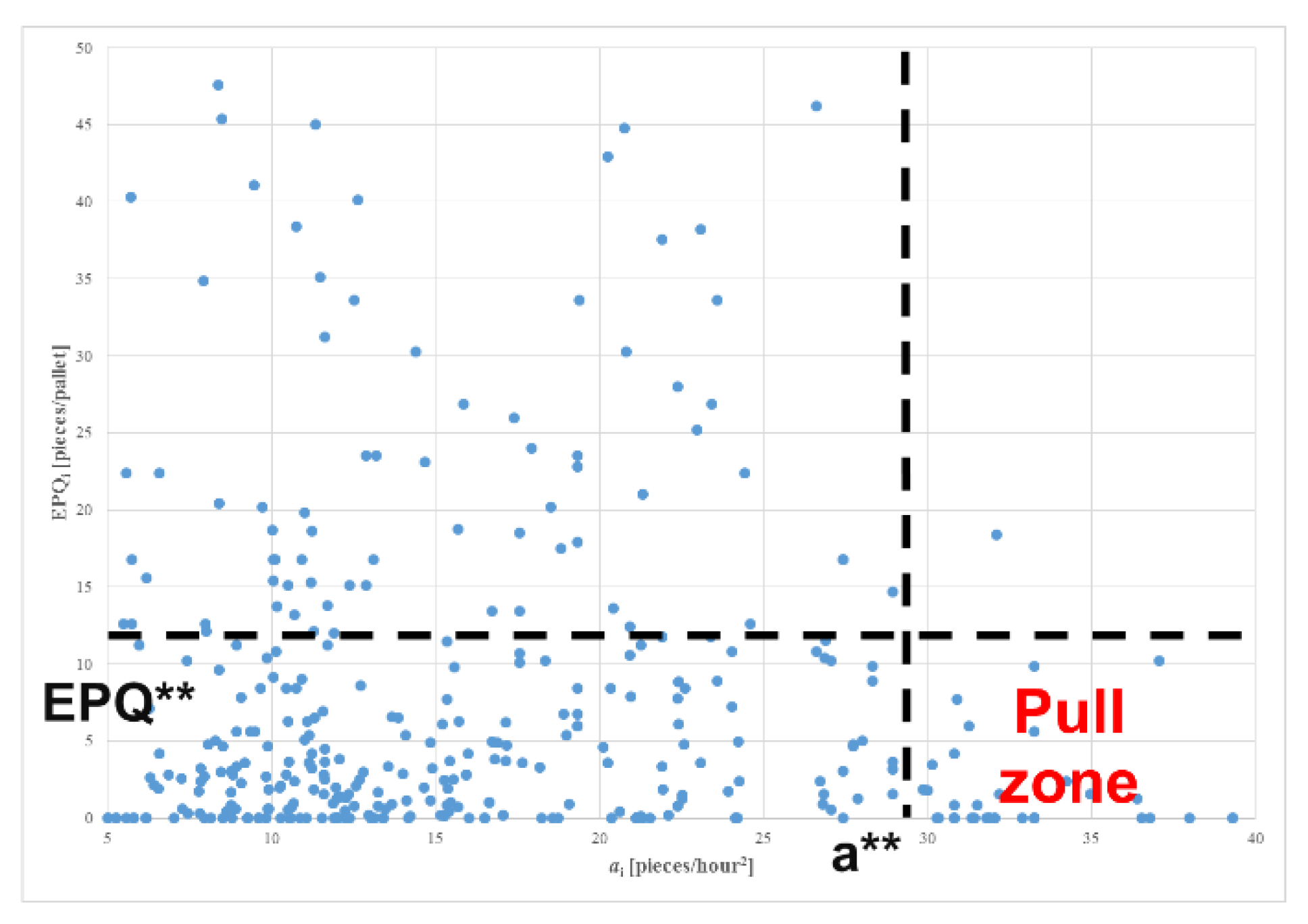
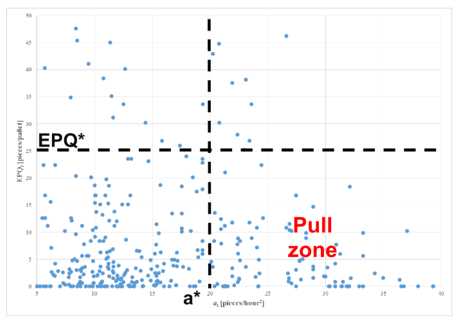
STEP 4. Final Push/Pull policy definition for each item. In this step, according to the breakeven optimal values of a** and EPQ**, it is possible to define the optimal Push/Pull policy to adopt for each part i. Figure 5 reports the case study values of a** and EPQ** compared with that of the different parts ai and EPQi, with related optimal Push/Pull policy to apply.

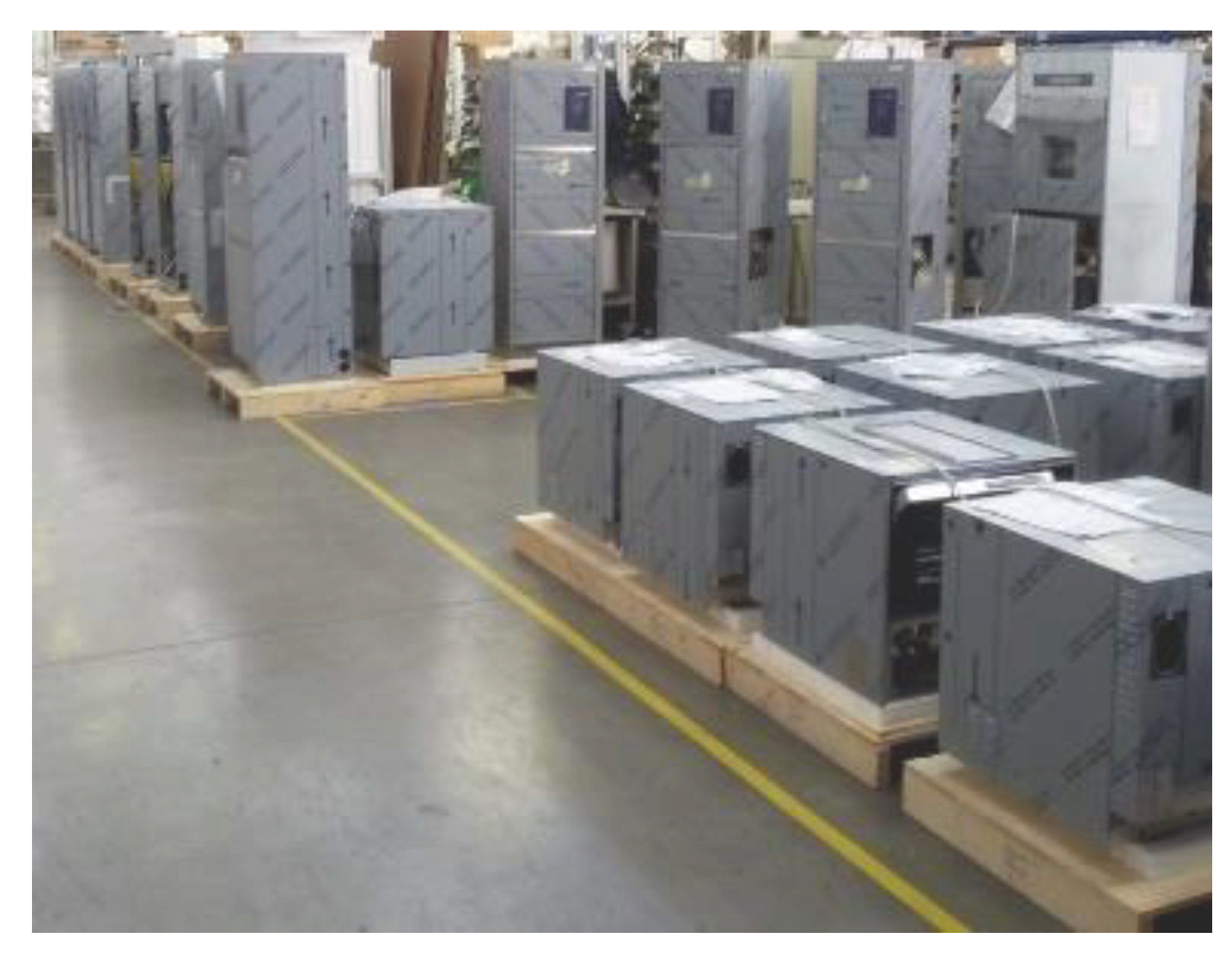
4. Case Study

The case study is referred to an Italian washing machine manufacturer. In the case study, the parts category where the proposed model for Push/Pull policy definition was applied are the metal sheet plate parts (as illustrated in Figure 6 and

Table 2. Case study $a_i$ and $EP{Q}_i$ values.

Item	ai	EPQi
660,622	30.2	28
7,086,197	10.3	6
806,614	45.5	28
100,635	34.2	536
100,645	10.4	112
100,708	91.3	112
806,615	58.4	28
110,616	12.9	20
100,622	13.7	22

). They are used as the product structure, generally used in the first assembly phases, and as product covers, which are generally used in the last assembly phases. They are interesting because:

• The production technologies used to produce these parts are cutting, bending, and welding. They are common, with not a high level of know-how.
• Their value can be considerable, especially if produced with high-value steels (i.e., stainless steel).
• They have a wide production mix (in terms of product variant dimension, shape, colors, etc.) since they are frequently used for the product customization.
• They are large and voluminous.

The last two points, considering a pure Push approach, negatively affect the inventory levels, with a potentially large occupation volume within the warehouse. For this reason, many industrial companies decide to include in their internal production the cutting, blending, welding, and if necessary, painting processes. A total of 425 internally produced parts are considered in the analysis, previously produced with an MTS-Push approach.

In this way it is possible to graphically define the position of each part according to the two parameters. The suitable parts for a Pull policy will be the parts with high values of $a_i$ and low values of $EP{Q}_i$. Figure 7 lists the 425 parts characterizing the industrial case study.

STEP 2. Multiscenario analysis. Considering different values of a* and EPQ* (as illustrated in Figure 7), the values of the two objective functions $P_{TOT}$ Equation (6) and $T{A}_{TOT}$ Equation (8) are assessed.

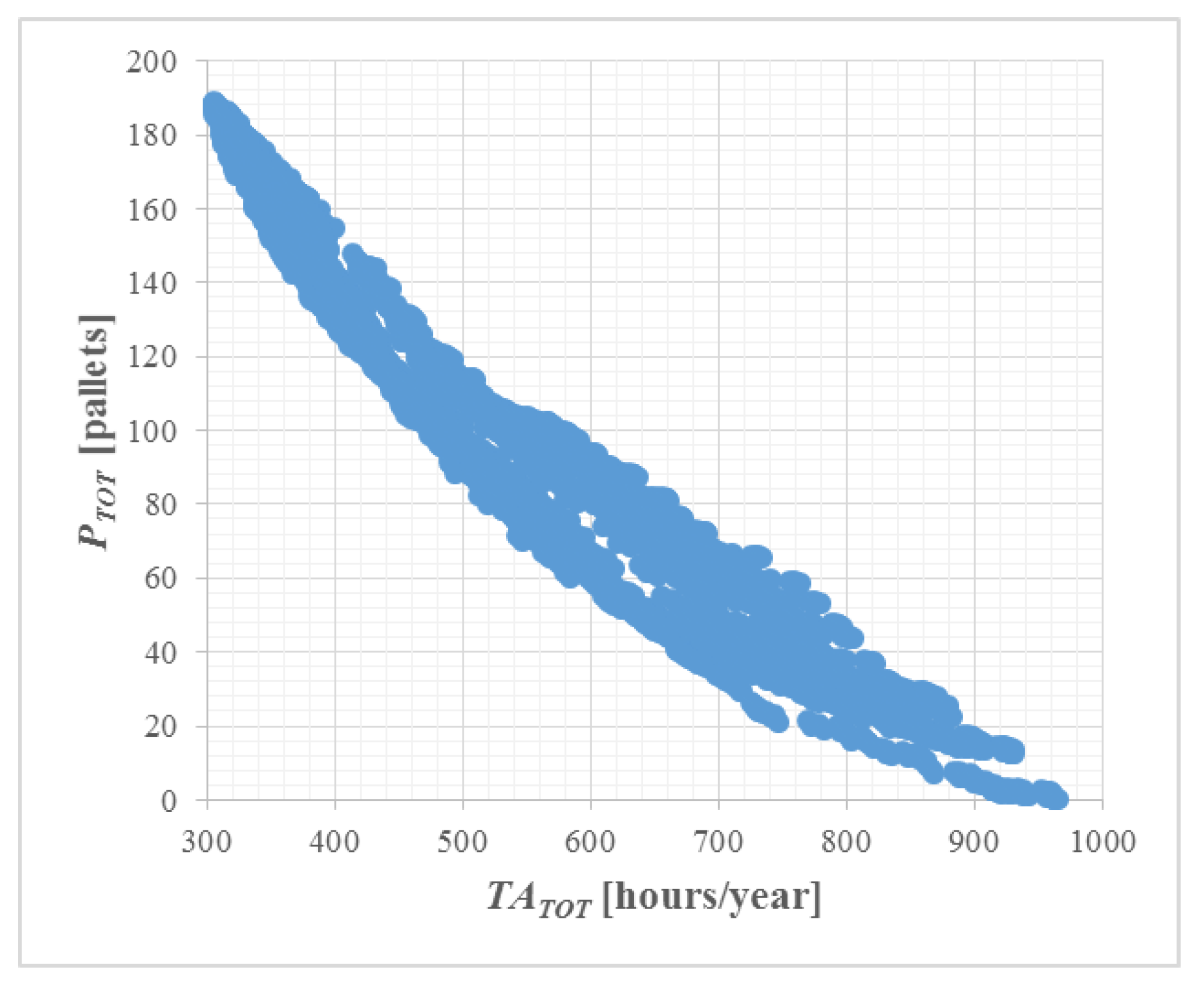
Main results are in Figure 8, where for each scenario the two objective functions values are plotted.

The procedure adopted to generate the different scenarios is detailed reported in Figure 2 (Step 2). From the computational point of view, the problem is trivial. The multiscenario analysis reported in Figure 4 was performed using Matlab SW with an Intel(R) Core i7 getting 2.88 × 10⁵ scenarios in 9.89 s.

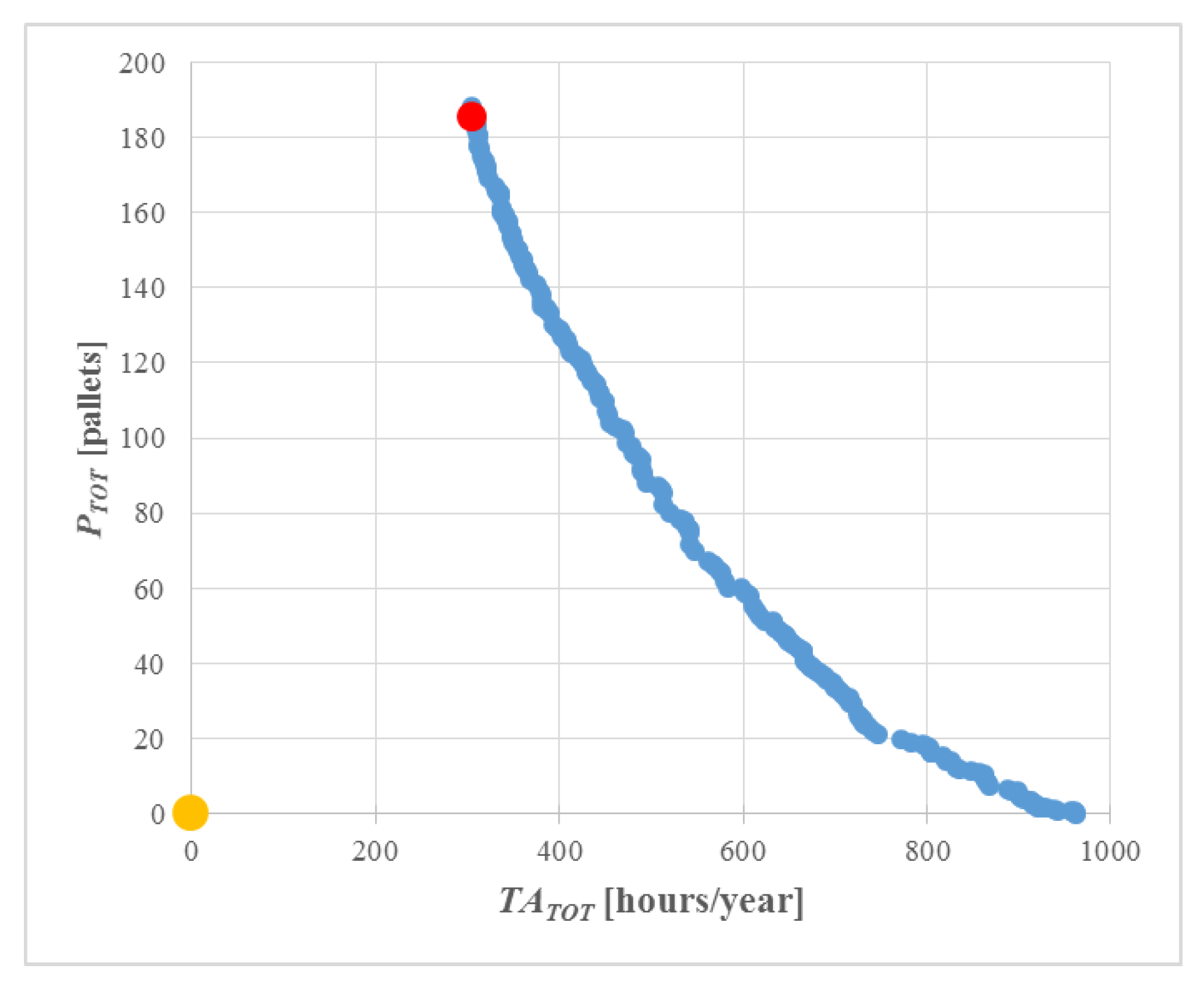
STEP 3. Construction of the Pareto Frontier of the optimal solutions and breakeven optimal parameters a** and EPQ** definition.

Figure 9 reports the Pareto Frontier of the case study, the set of solutions where no other solution dominates them. At this stage, the decision maker needs to select an optimal bi-objective solution $(\overline{\overline{T{A}_{TOT}}};\overline{\overline{\overline{P_{TOT})}}}$ among the set of dominant points. To find the bi-objective optimal point, the minimization of the Euclidean distance between the Utopia point and the points belonging were applied Equation (11). In Figure 9, the bi-objective optimum point (in red) within the Pareto frontier (in blue) compared to that of the Utopia point (in yellow) is reported.

The bi-objective optimum point Equation (11) is:

$(\overline{\overline{\mathit{T}{\mathit{A}}_{\mathit{T}\mathit{O}\mathit{T}}}};\overline{\overline{\overline{{\mathit{P}}_{\mathit{T}\mathit{O}\mathit{T}})}}}$ = (305.72; 185.25).

Once defined it, it is possible to derive the breakeven optimal values of a** and EPQ** of the related scenario that are a** = 29.75 pieces/h2 and EPQ** = 12 pieces/pallet.

STEP 4. Final PUSH/PULL policy definition. In this stage, according to the breakeven optimal values of a** and EPQ**, it is possible to define the optimal PUSH/PULL policy to adopt for each part i. Figure 10 reports the case study values of a** and EPQ** compared with that of the different parts ai and EPQi, with related optimal PUSH/PULL policy to apply.

The application of the proposed procedure to the plate parts of the case company moved 29 parts of 425 from Push to Pull policy (about 7%). In this hybrid Push/Pull scenario, compared with that of the previous pure Push policy, the total number of stocked pallets at the warehouse decreases by about 27%, while the total setup time increases by about 3.5%. The results demonstrate that the application of the proposed bi-objective optimization model reduces the stocked pallet.

On the other hand, the increase in setup time is lower than in the parts moved from Push to Pull Policy (3.5% versus 7%).

To validate the proposed approach, the case study data are used, comparing the obtained solution toward a milestone MTO/MTS production method: the economic production quantity [34]. The economic production quantity model (EPQ) determines the quantity a company needs produce to minimize the total inventory costs by balancing the inventory holding cost and average fixed ordering cost. The formulation of the EPQ is known and not reported in the paper for the sake of brevity.

Moreover, the single-objective solutions $P_{TOT}$ and $T{A}_{TOT}$ are reported as well. The single objective solutions aims to minimize only one of the objective functions.

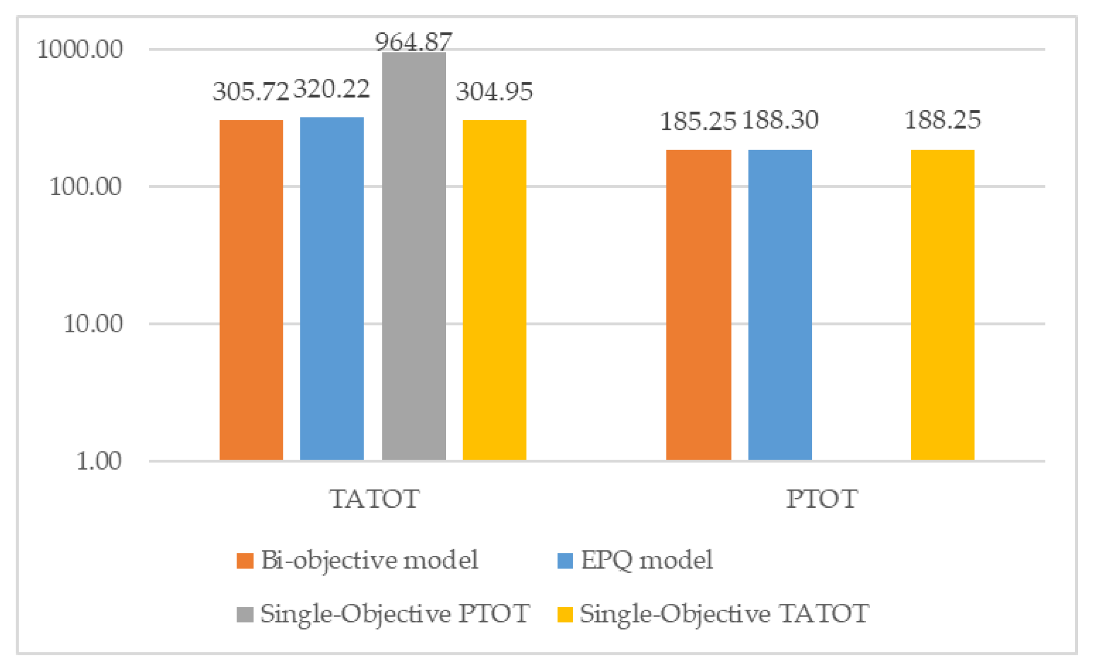
Figure 11 shows the two-basic function $P_{TOT}$ and $T{A}_{TOT}$ calculated for the two methods. (EPQ versus the proposed bi-objective method). The Scenario proposed by the EPQ model is a dominated solution respect the Pareto Frontier. As consequence, both the objective functions are in this case greater than the optimal solution proposed but the bi-objective model. In fact, the case study is composed by many large parts, with even low demand. As a consequence, the EPQ model has a certain number of items with production batch equal to 1 with a high impact on the setup times. On the other hand, EPQ proposes items with large production batches and high space utilization. As shown in Figure 11 the proposed bi-objective methodology performs better than EPQ for the considered case study.

Looking at the single-objective functions, it was reported that solutions lie on the Pareto frontier. There can be solutions with the same values of one objective function but greater values of the other. The proposed bi-objective methodology performs better by considering both objective functions at the same time. As shown in Figure 11, with a small increase in one objective function, it is possible to obtain a large decrease in the other.

5. Conclusions

The paper aims to propose a bi-objective mathematical model for the optimization of the produced parts according the MTS/MTO policy. The procedure aims to minimize both the setup time and the storage used space. The case study is referred to the plate parts. The proposed model can easily apply to other parts categories. The model is based on a step-by-step procedure. The inventory parameter $EP{Q}_i$ (number of maximum storable piece in an EPAL) and the production parameter $a_i$ (agility) are calculated for each part. According the two objective functions, Total Setup Time and Total EPAL Stored, the bi-objective optimal point is calculated through the Pareto frontier definition and through the minimal distance to the Utopia point. Finally, according to this optimal value of the two objective functions, the breakeven values of the inventory and production parameters a** and EPQ** are defined.

The results demonstrate how the application of the bi-objective optimization model generates a scenario where an important inventory saving is reached, allowing a quick response to the order changes without impacting production. Future research will focus on the extension of the model, where the agility concept is extended also to the supply chain, considering the purchase-to-order versus the purchase-to-stock policies and the related variables and constraints. Moreover, the process variability can be considered in the optimization model, including, for example, variable setup times.