Resilient Scheduling as a Response to Uncertainty in Construction Projects

Abstract

Complex construction projects are developed in a dynamic environment, where uncertainty conditions have a great potential to affect project deliverables. In an attempt to efficiently deal with the negative impacts of uncertainty, resilient baseline schedules are produced to improve the probability of reaching project goals, such as respecting the due date and reaching the expected profit. Prior to introducing the resilient scheduling procedure, a taxonomy model was built to account for uncertainty sources in construction projects. Thence, a multi-objective optimization model is presented to manage the impact of uncertainty. This approach can be described as a complex trade-off analysis between three important features of a construction project: duration, stability, and profit. The result of the suggested procedure is presented in a form of a resilient baseline schedule, so the ability of a schedule to absorb uncertain perturbations is improved. The proposed optimization problem is illustrated on the example project network, along which the probabilistic simulation method was used to validate the results of the scheduling process in uncertain conditions. The proposed resilient scheduling approach leads to more accurate forecasting, so the project planning calculations are accepted with increased confidence levels.

1. Introduction

Large construction projects are characterized by their complexity in terms of organization, as they consist of hundreds of activities and require numerous resources. To successfully manage important project objectives, scheduling efforts must be applied to ensure that a project is completed within the contract requirements [1]. Schedule management concentrates on the processes that are essential to appropriately deliver critical project aspects, such as time, cost, resources, etc. [2] Scheduling methods which are used to establish reliable construction plans can be broadly classified into exact [3,4,5,6], heuristic [7,8,9], or metaheuristic approaches [10,11,12,13,14]. Current practices in the domain of construction planning and scheduling are oriented towards automatic schedule development and the application of specialized optimization techniques [15]. Although modern technologies such as BIM have already been applied to the optimization problems in the realm of construction scheduling [16,17,18,19,20,21], additional development and possible extensions are still needed to effectively automatize scheduling practices and improve both customizability and user-friendliness of emerging technologies for practical use [22,23].

As construction projects take place in a dynamic environment, they are consequently prone to the negative impacts of internal and external sources of uncertainty. Due to the fact that uncertainty has been recognized as a cause of risks that can influence the final outcome of a project [24], there is an indisputable need to manage the uncertainty which is present in almost all of the construction activities [25]. However, there is still a lack of mechanisms that would leverage state-of-the-art technologies such as BIM with the uncertainty management frameworks in complex construction projects [26]. BIM-based uncertainty management frameworks are currently emerging at the theoretical level, where the automatization and practical integration of existing frameworks with new technologies remain the main challenges thus far [27].

To diminish unfavorable impacts stemming from the construction project environment, a relevant strategy is to prepare for uncertainty from the early stages of the project life cycle. To account for uncertainty as early as in the project planning phase, a resilient scheduling approach has been developed recently [28,29,30]. Resilient scheduling is a procedure to develop the optimal baseline makespan for a project, considering the trade-off between schedule stability or robustness, and other important objectives, such as makespan minimization [29]. Moreover, additional trade-offs can be considered when defining the equilibrium state of the project, such as the limited budget of the project, expected net present value, as well as adequate risk management, among other equilibrium facets [28].

Resilient schedules are defined by their multidimensionality: they tend to be robust, flexible, and adaptable. Previous studies in construction scheduling have predominantly focused on the robustness aspect, which is already a complex concept. On the one hand, robustness depicts the insensitivity of objective function in the optimization model, may it be project minimization or NPV maximization, for example; on the other hand, it tends to minimize the deviations between baseline schedule and realized state. For instance, Zhao et al. [31] propose the framework for integrated robustness evaluation, considering composite robustness measure. Authors have been using improved subjective and objective weights in order to evaluate the schedule robustness. In another research, Zhao et al. [32] investigated the importance of schedule robustness by use of metaheuristic optimization techniques, considering both activities’ starting-time deviation, as well as a structural deviation in a schedule.

On the other hand, information about the uncertainty in a construction project is usually scattered, as it arises from various sources, and due to the dynamics of complex construction projects, it is extremely demanding to organize, collect, and reuse that knowledge. Lack of information or ambiguous data can have undesirable consequences on project success and cause a negative impact to project objectives. According to Reference [33], significant efforts have been undertaken to consider more general sources of uncertainty in the project management domain. Because of the inherent complexity in large construction projects, there is a need to manage a considerable amount of information [34].

In the realm of construction management, different researchers have attempted to integrate knowledge about uncertainty into formal conceptualization. This way, domain knowledge can be accessed and reused by users in a form of computer-readable data [35]. For example, Tah and Carr [36] proposed a knowledge-based approach to facilitate effective risk management procedures in a construction project. Ping Tserng et al. [37] developed an ontology-based risk management framework to improve the overall effectiveness of risk management practices for a construction contractor. The study of Ding et al. [38] coupled ontology and semantic web technology in a BIM environment to manage construction risk knowledge. Apart from enhancing general risk management procedures, other practical applications of ontology in the construction domain include knowledge sharing [39,40,41], information extraction [42,43,44], and performance analysis [45,46,47,48].

So far, however, there has been little discussion about modeling a comprehensive knowledge base by considering general sources of uncertainty in construction projects. Therefore, the first aim of this research was to structure uncertainty sources related to complex construction projects in a faceted taxonomy, as a basis for the analysis and uncertainty management in construction projects from the early planning stages. Comprehensive identification and characterization of uncertainties in the construction domain is a first step towards increasing the probability of reaching project goals during the execution phase.

Considering the nature of complex construction projects, which are financially extremely demanding undertakings, appropriate cash procurement is of vital importance. The major source of financing for construction projects is the establishment of the bank overdraft [49,50]. If the cash deficit occurs during the project realization period, contractors will encounter difficulties related to the implementation of the project activities in accordance with a baseline plan [51]. Therefore, the development of a schedule where the cash flows will be suitable for the established bank overdraft is an important subject, since large construction projects require extensive investments and rarely depend solely on the savings of the contractor [49,50].

The main objective of this research is to propose a comprehensive mathematical model for resilient scheduling as a trade-off between project robustness, project duration, and contractor’s profit. Previous studies on resilient project scheduling [28,29,30] have not dealt with the finance flow modeling, so the mathematical problem presented in this study aims to contribute to the growing area of research on resilient baseline scheduling by introducing the additional objective function for profit maximization at the end of the project. The present research contributes to a more practical setting in the context of resilient construction scheduling by including the financial aspect in the existing problem. In this way, we assess the issue of financial feasibility in resilient scheduling for construction projects.

2. Resilience Approach to Manage Uncertainty in Construction Projects

The methodological approach taken in this research is presented as an algorithm for resilient scheduling to manage uncertainty in construction projects, as depicted in Figure 1. At the start, uncertainty sources in a construction project are analyzed to clarify how uncertainty impacts project objectives. From here, the multi-objective optimization (MOO) model is developed to serve as a response to uncertainty in construction projects. The objective functions in the model stem from the uncertainties related to variability in the durations of activities. In such a way, the optimization method overcomes problems of the deterministic approach which cannot account for activities’ completion times with absolute certitude. The optimization problem consists of three objective functions and complementary constraints. Decision variables in the MOO model define the start times for activities in a project once the optimization problem is solved by the use of a hierarchical approach. The solution is obtained in a form of a resilient baseline schedule. Finally, the baseline schedule is validated by the simulation analysis, where recognized uncertainty sources are modeled as stochastic variables.

The structure of this study is organized as follows. The following subsection begins with a discussion on the nature of uncertainty in construction projects. In Section 2.2, the taxonomy development process is described. Resilience framework is discussed in more detail in Section 2.3. In Section 2.4, the MOO model for resilient scheduling is presented. The Section 3 consists of two parts, where the solving process is discussed in more detail in Section 3.1, while the resilient scheduling approach is validated on the construction project example by simulating two baseline cases in Section 3.2. The overall conclusions and suggestions for future research are given in Section 4.

2.1. Understanding Uncertainty

During the execution phase, many undesirable events might affect project constraints, such as budget overrun or timely execution of significant project activities. Disruptions in a project schedule due to mechanical malfunctions or unfavorable meteorological conditions on site could cause delays in project makespan unless managed properly. Occurrence, as well as the impact of disruptive events on project objectives, is uncertain; therefore, it is important to understand sources of uncertainty in a construction project.

Some authors consider uncertainty as various undesirable conditions or events, e.g., unpredictable resource unavailability, changing environmental conditions, various user needs, and system intrusions or faults [52]. Further examples of uncertain events include an increase in material prices, an accident during construction, a decision-maker’s change of mind, etc. [53]. The corresponding perspective was adopted in this study, defining uncertainty as a high variety of possible events and conditions that could occur and affect project objectives.

Previous research has revealed certain characteristics considering the uncertainty in construction projects. For example, Gündüz et al. [54] reported that most of the uncertainty sources can be traced to conditions and events on site. Authors discovered that from 83 identified uncertainty factors that could delay construction performance, over 90% were traceable to the activities within the construction site. On the other hand, considering the time distribution of uncertainty through the project’s life cycle, Ustinovičius [55] concluded that in the initiation phase the majority of uncertain events and conditions could be expected. When it comes to the classification of uncertainty sources, various perspectives are emerging from different studies in the project management domain. Most of the research work categorizes uncertainties in two major categories: internal or external, while both of the categories could be further extended into subcategories, such as technical, commercial, environmental, socioeconomic, political, etc. [56]. Since most studies in the construction domain have only focused on certain aspects of uncertainty analysis, such as uncertainty related to the specific phase of a project [55], or uncertainty related to the particular objective of a construction project [56], this paper aims to discuss a conceptual method based on the comprehensive literature review to accumulate, process, and reuse the dispersed knowledge on uncertainty, considering different aspects of a construction project. The following section aims to explain the process of development for the structured and systematic knowledge base of uncertainties, considering construction projects.

2.2. Taxonomy

Herein, a voluminous body of information is deliberately omitted, aiming to present only the fundamental principles in the process of creating the taxonomy model. Taxonomy is modeled by the use of the open-source platform Protégé. The taxonomy model serves as a basis for modeling the impact of uncertainty on baseline schedules in the final step of resilient schedule validation. In this study, the taxonomy model is a representation of domain knowledge by the use of concepts organized into facets and/or hierarchical structures. In the multifaceted taxonomy, every facet represents different features of the concept which is classified [57]. For example, one facet embodies uncertainties considering project life-cycle phases, and the other depicts uncertainties regarding stakeholders in a construction project, etc. Each of the facets could be further described by an independent taxonomy [57], either in hierarchical, faceted, or combined form.

The taxonomy model is developed to account for a high variety of possible events and conditions that could occur and affect project objectives. As the main objective is the development of construction schedules that are resilient to disruptions stemming from uncertainties, the starting point, i.e., universe of discourse of the taxonomy, is determined as “Uncertainty sources in a construction project”. The main concept is further depicted by sub-concepts, i.e., facets, which ought to exhaustively describe the universe of discourse.

Faceted systems are in their nature general knowledge management models based on a multidimensional classification of heterogeneous data [57]. Since different authors argued sources of uncertainty in construction projects in a constrained way, e.g., solely with impact on transaction cost [56], multifaceted classification was imposed on the representation of the gathered knowledge.

The main concept is depicted by sub-concepts, i.e., facets, which ought to exhaustively describe the universe of discourse. To maintain integrity while modeling sub-dimensions (facets) of the main concept, fundamental categories were developed by following the core principles of knowledge organization, referring to five fundamental categories of knowledge classification [58], as presented in

Table 1. Fundamental facets for the uncertainty sources in a construction project.

Abstraction Category	Facet Question	Facet	Description
Personality	Who	Member	Uncertainty related to the member in a construction project.
Matter	What	Project	Uncertainty related to a construction project itself.
Energy	How	Impact	Uncertainty impact on the project objective.
Space	Where	Cause	Cause of uncertainty source in a construction project.
Time	When	Life cycle	The time dimension of a construction project presenting a stage when uncertainty may arise.

.

The facets are revealed through the literature review, and they tend to describe the main concept exhaustively. To prevent ambiguity or vagueness of any kind, we offer five main facets:

• Member facet tends to describe all aspects of human attributes together with their mutual relationships which could lead to project perturbations. Members in a construction project could be individuals as well as groups of people, i.e., organizations.
• The project is described as features of a construction project which represent substantial means of how a project affects uncertainty existence.
• Impact means all the direct effects of uncertainty sources on traditionally determined project objectives (schedule-budget-quality goals), with additional sustainability aspects [59].
• Causes are states, conditions, and events in which sources of uncertainty are triggered.
• The life cycle presents stages of a construction project in which uncertainties may arise. This facet is the time dimension of the universe of discourse.

The structure of five main facets further depicted with the second-level entities (sub-facets) is shown in

Table 2. The second level of faceted hierarchy for uncertainty sources in a construction project, where the primary node is “Uncertainty sources in a construction project”.

Member	Project	Impact	Cause	Life Cycle
Behavior	Activities	Cost	Location	Conceptualization
Capacity	Complexity	Quality	Threats	Planning
Decision making	Novelty	Schedule	Type	Execution
Interactions	Type	Sustainability	-	Termination
Nature	-	-	-	-

Full taxonomy model is available upon request from the corresponding author.

. Currently, the taxonomy model counts more than 300 entities in the form of mutually categorized terms, accompanied by the definition for each term to prevent any ambiguity. While the main idea of classification is to systematically represent the integrity of the source term, compounding terms is the process of composing different concepts to form a distinct term. For example, the term “Crane failure due to mechanical malfunctions or breakdowns” is compounded from concepts “Resources” and “Breakdowns”, so there is no need to explicitly denote the existence of the compound term. Due to the complexity of the task, it is on the final users of taxonomy to validate possible combinations of uncertainty sources in construction projects.

The presented taxonomy model in a comprehensive, yet restricted manner describes uncertainty sources in a construction project. The uncertainty assessment plays an important role in the overall approach to model resilient schedules since the detailed examination of uncertainty sources is needed to recognize the impact on project objectives. Therefore, this taxonomy reveals the fundamental need to cope with unfavorable disruptions in the process of creating a baseline schedule. As a next step in the overall methodology, resilient scheduling is deployed to produce stable makespans for construction projects under the impact of uncertainty.

2.3. Resilience as a Response to Uncertainty in Construction Projects

Herein, we propose the procedure based on the resilient scheduling concept and optimization modeling to manage uncertainty in a construction project and develop a construction schedule resilient to disruptions. The resilience strategy to cope with uncertainties is to recognize them as early as possible, namely in the project planning phase. By doing this we reduce the number and intensity of disruption shocks during the project implementation. Resilient scheduling, together with early identification of the uncertainties, plays a crucial role in reducing the risks of the construction projects. The main goal of resilient project scheduling is to maximize the preservation of the project baseline schedule at the equilibrium state during project execution. The concept of equilibrium state generally refers to timely project completion and minimized project tardiness amount, considering both project due date and activities’ start times when executed activities are compared to a baseline schedule [28]. In this study, we extend the concept of equilibrium state by examining the degree of credit limit preservation and achievement of the baseline profit goal.

The goal of the proposed approach is to obtain the proactive baseline schedule as a response to the impact of uncertainty, from the contractors’ perspective. As illustrated in Figure 2, the research procedure consists of three main parts. The starting point is identification, evaluation, and interpretation of uncertainty sources by the systematic literature review and also by using the developed taxonomy to avoid ambiguity and vagueness. The systematic literature review in this study was done by following the process for uncertainty identification and classification from Warmink et al. [60]. This way, the taxonomy serves as an essential tool for contractors to manage uncertainty in the planning phase, in view of the knowledge extraction and reuse during the optimization process. However, by finding new concepts during the identification process, the taxonomy is being constantly updated. The second phase in the proposed method is oriented toward solving the multi-objective optimization problem, where objective functions capture uncertainties. In this paper, we show an optimization model for resilient scheduling problem with three objective functions that strive to simultaneously (i) minimize project duration, (ii) maximize the level of resilience built in the baseline schedule, and (iii) maximize profit from the contractors’ perspective.

The detailed finance framework is incorporated into the problem of resilient baseline scheduling so the cash flows can be calculated throughout the duration of a project. The model is built from the contractors’ perspective to ensure the financial feasibility of a baseline schedule. In the case of a cash deficit, the contractor is threatened with the possibility of impeded work on the construction site. The interrupted workflow could lead to significant delays and eventually to additional overheads and liquidated damages and, hence, lower profit [51]. Since the appropriate financing of the construction project is of the utmost importance when it comes to the timely execution of project activities, the research hypothesis is that the contractor will be able to reliably commit to the baseline schedule if the final profit is maximized. Project profit maximization indicates reduced overhead expenses, so the overall project cost is minimized; therefore, project performances are improved to benefit all stakeholders. This way, the additional layers of adaptability and flexibility are implicitly included in the mathematical model by realistically calculating cumulative cash flows throughout the project makespan.

In the following step of the proposed procedure, the optimization process is conducted for the resilient scheduling problem, and the result is obtained in the form of a baseline makespan, by determining the optimal start time for each activity.

2.4. Optimization Model for Resilient Scheduling Problem

This section describes the optimization model for creating a feasible, resilient baseline schedule. Details related to the resilience improvement through surrogate measure maximization are discussed in the following subsection, followed by the statement of the mathematical problem in Section 2.4.2.

2.4.1. Surrogate Measure and Activity Weights

The concept of resilient scheduling is built on the idea of providing enough time intervals in the initial baseline structure so the schedule is able to absorb disturbances caused by the impact of uncertainty. A common approach is to provide enough time floats in the initial solution by the use of different surrogate measures [28,29,30,61,62]. This way, the stability of a schedule is approximated under the low cost of computational complexity, providing a simple solution in the overall computationally demanding optimization process.

The surrogate measure in this study is modeled as a weighted sum of resource-technology free floats [30] of all activities in a project. The resource-technology free float (${\mathrm{FF}}_{\mathrm{i}}$) calculates the amount of time for which an activity can be prolonged without postponing start times of succeeding activities, in a way that both precedence and resource relations are considered. On the other hand, activity weights ($w_i$) are significant for appropriate float distribution, since they express the relative importance of the${\mathrm{FF}}_{\mathrm{i}}$. For activities with the higher weight (w_i), it is more important to provide bigger FF_i, so the baseline schedule is as resilient as possible. Activity weight is calculated based on four indices:

• AS_i—Equation (1) states the relative number of successors per activity. The number of direct and indirect successors (N_succ) for the activity i is divided by the number of all activities in a project, n (both dummy start and dummy end included);
• DP_i— Equation (2) calculates relative duration of the activity, i;
• AC_i— Equation (3) determines relative cost of the activity, i;
• RU_i— Equation (4) counts relative resource usage as required by the activity, i.

The assumptions are as follows: (i) with an increased number of successors, there is a higher probability to propagate time disruptions through the baseline schedule; (ii) activities that are expected to be executed during a longer time have a higher probability of disruption; (iii) the higher the cost of the activity, the bigger is the impact to the cash flow of a project; and (iv) with higher resource consumption, there is a higher probability of resource breakdown. Therefore, the activity weight ($w_i$) is calculated as follows:

$$A{S}_i=\frac{N_{succ}}{n}$$

(1)

$$D{P}_i=\frac{d_i}{{\sum }_{i=1}^n{d}_i}$$

(2)

$$A{C}_i=\frac{c_i}{{\sum }_{i=1}^n{c}_i}$$

(3)

$$R{U}_i=\frac{{\sum }_{r=1}^k{u}_{ir}}{{\sum }_{i=1}^n{\sum }_{r=1}^k{u}_{ir}}$$

(4)

Finally,

$$w_i=\frac{A{S}_i+D{P}_i+A{C}_i+R{U}_i }{4}$$

(5)

Multiplication of ${\mathrm{FF}}_{\mathrm{i}}$ by the activity weight ($w_i$) accounts for proper float distribution in the baseline schedule, aiming to preserve the project at the equilibrium state. Therefore, by maximizing the weighted sum of the resource-technology free floats, the resilience of the initial makespan is improved.

2.4.2. Optimization Problem

The optimization model presented in this study is based on the existing bi-objective resilient scheduling problem [30], which is improved by introducing the additional objective function to maximize the profit from a contractors’ perspective. This way, an additional layer of financial stability is provided in the project baseline structure. With the net profit increase, the hypothesis is that contractor is fit to make financial compensation for perturbed activities. This means that adaptability to project disruptions is enhanced by maximizing the third objective function in the model. Moreover, the credit limit is included as one of the constraints in the optimization model, thus ensuring the financial feasibility of the optimal baseline schedule. A credit limit is imposed to assure that a financial flow is bounded to an allocated cash amount through the entire execution of the project.

In addition, the methodology of activity weight calculation is introduced. This way, the surrogate measure is appropriately quantified so the resilience of a schedule can be approximated in the optimization process. Activity weight calculation is inspired by the work of Torabi Yeganeh and Zegordi [29], where the weight of each activity is determined based on resource usage, network complexity, and time overlap. For this study, the additional layer concerning the direct cost of each activity was combined with the existing factors to quantify the activity weights.

Table 3. Parameters and sets used in the optimization problem.

Symbol	Description
T	Length of the planning horizon (t = 1, 2, …, m)
A	Set of project activities (i = 1, 2, …, n), including dummy start 0 and dummy end n + 1
E	Set of precedence relations
R	Set of project resources (r = 1, 2, …, k)
${\mathrm{w}}_{\mathrm{i}}$	Weight of activity i
${\mathrm{d}}_{\mathrm{i}}$	Expected duration for activity i
${\mathrm{c}}_{\mathrm{i}}$	Deterministic cost of activity i
${\mathrm{u}}_{\mathrm{ir}}$	Consumption of resource r as required by activity i
${\mathrm{a}}_{\mathrm{r}}$	Availability of resource r during project time T
${\mathrm{FF}}_{\mathrm{i}}$	Resource-technology free float for activity i
$\mathrm{P}$	Final profit at the end of a project
$\mathrm{EOM}$	End of the month considering project timeline (time step used when calculating Cash Flow), (EOM = 1, 2, …, l)
${\mathrm{CG}}_{\mathrm{l}}$	Cumulative cash flow value at the end of the month l
$\mathrm{W}$	Credit limit for the project

summarizes the notation used in the optimization model. In the optimization model, binary decision variables were used to calculate activity start times, where $x_{it}=1$ if activity, i, starts at the time, t; otherwise, $x_{it}=0$.

The multi-objective optimization model (MOO) for resilient baseline scheduling in construction projects is expressed as follows:

$$\mathrm{Min} {\displaystyle \sum }_{\mathrm{t} \in \mathrm{T}}\mathrm{t} \times {\mathrm{x}}_{\mathrm{n}+1,\mathrm{t}}$$

(6)

$$\mathrm{Max} {\displaystyle \sum }_{\mathrm{i} \in \mathrm{A}}\left({\mathrm{w}}_{\mathrm{i}}\times { \mathrm{FF}}_{\mathrm{i}}\right)$$

(7)

$$\mathrm{Max} \mathrm{P}$$

(8)

Subject to:

$${\displaystyle \sum }_{\mathrm{t} \in \mathrm{T}}{\mathrm{x}}_{\mathrm{it}}=1, \forall \mathrm{i} \in \mathrm{A}\cup \left\{0, \mathrm{n}+1\right\}$$

(9)

$${\displaystyle \sum }_{\mathrm{t} \in \mathrm{T}}\mathrm{t} \times {\mathrm{x}}_{\mathrm{it}}\le {\displaystyle \sum }_{\mathrm{t} \in \mathrm{T}}\mathrm{t}\times {\mathrm{x}}_{\mathrm{jt}}-{ \mathrm{d}}_{\mathrm{i}}, \forall \left(\mathrm{i},\mathrm{j}\right)\in \mathrm{E}$$

(10)

$${\mathrm{CG}}_{\mathrm{l}}\le \mathrm{W}; \forall \mathrm{l} \in \mathrm{EOM}$$

(11)

$${\displaystyle \sum }_{\mathrm{i}=1}^{\mathrm{n}}{\displaystyle \sum }_{\mathrm{q}=\max \left\{0, \mathrm{t}-{ \mathrm{d}}_{\mathrm{i}}+1\right\}}^{\mathrm{t}}{\mathrm{u}}_{\mathrm{ir}}\times {\mathrm{x}}_{\mathrm{iq}}\le {\mathrm{a}}_{\mathrm{r}}, \forall \mathrm{t} \in \mathrm{T}, \forall \mathrm{r}\in \mathrm{R}$$

(12)

$${\mathrm{x}}_{\mathrm{it} }\in \left\{0, 1\right\}, \forall \mathrm{i} \in \mathrm{A}\cup \left\{0, \mathrm{n}+1\right\}, \forall \mathrm{t} \in \mathrm{T}$$

(13)

The first objective function, shown in Equation (6), minimizes the start time for dummy end activity, minimising the project duration in total. Multiplication of binary variable $x_{it}=1$ with specific time step (t) defines the start of activity (i) at the start time, t, supposing that time, t, corresponds to the start time of activity (i) from the baseline solution. For all other time steps, the binary variable $x_{it}$ equals 0, as stated in the constraint part of the model. The second objective function, as stated in Equation (7) maximizes resilience through the surrogate measure (SM), which is represented by the sum of weighted resource-technology free float [30] for each activity, as explained in the previous subsection. The third objective function, shown in Equation (8), maximizes profit for the contractor at the end of the project by maximising the cumulative cash flow of dummy end activity. Constraint expressed in Equation (9) ensures that each activity, including the dummy start and end, can be started only once. Precedence constraint is expressed in Equation (10), defining that no activity can start before the precedent one is finished, for all activities that belong to the set of precedence related pairs. Financial constraint is shown in Equation (11) and it states that at the end of each month, the cumulative cash gap (before receiving the payment from the investor) must not exceed the permitted credit limit. Resource constraints are specified in Equation (12) by considering all possible start times, $x_{iq}$, for all activities (i) such that activity is in progress in period q, for every time step, t, and every resource, r. Multiplication of binary variable $x_{iq}$ with resource consumption ${ \mathrm{u}}_{\mathrm{ir}}$ must not exceed resource availability, ${\mathrm{a}}_{\mathrm{r}}$. Constraint which is stated in Equation (13) defines the decision variable as a binary one.

Financial flow is modeled from the contractors’ perspective by equations used in the work of Elazouni and Metwally [49] that, in turn, rely on the financial terminology clarified by Au and Hendrickson [63]. Since the bank overdraft has been recognized as a prevailing method for financing construction projects [49,64,65], this study also considers the bank overdraft as a single source of financing the construction project. For this reason, the cash-flow model in this study adopted established calculation [49] and incorporated two adjustments to improve the validity of financial flows. The first modification refers to the inclusion of interest rate, h, which rewards the contractor with an interest paid for positive cash flow. The interest rate (h) applicable on positive balances is less than the interest rate, ir, charged for borrowing in the case of a negative cash balance for the contractor [66]. The second adjustment is applied to explicitly display the return of the retainage amount at the end of the project. By modeling the retainage amount as an absolute value, it is assured that a contractor receives complete payment from an investor. Notation for required input variables to model financial flow is presented in

Table 4. Input variables required for financial flow modeling.

Symbol	Description
${\mathrm{d}}_{\mathrm{i}}$, $\mathrm{i}\in \mathrm{A}$	Duration of activities
${\mathrm{s}}_{\mathrm{i}}$, $\mathrm{i}\in \mathrm{A}$	Start times for activities from baseline schedule
${\mathrm{c}}_{\mathrm{i}}$, $\mathrm{i}\in \mathrm{A}$	Total direct cost per each activity in thousand of financial units
OP	Overhead percentage in decimal form
MP	Mobilization percentage in decimal form;
TP	Tax percentage in decimal form
MP	Markup percentage in decimal form
BP	Bond percentage in decimal form
N	Negotiated duration of the project in months
S	Realized duration of the project in months
ADV	Advance payment (percentage of TBP in decimal form)
D	Late completion penalty in thousand of cost units
RET	Percentage of retainage for investors’ payments (decimal)
ir	Interest percentage in decimal form
h	Surplus percentage in decimal form (h < ir)
k	Percentage for interest on the unused portion of a credit
W	Specified credit limit of the overdraft

.

It is assumed that receipts from the investor lag one month after realized expenses. Effects of financing costs are considered and calculated as seen in Reference [49], with two adjustments as previously described. The goal of finance flow modeling is to determine accurate values for the maximal cash gap (CG) and final profit for the contractor (P) for a particular instance of the baseline schedule. In the work of Elazouni and Metwally [49], the mentioned output variables of interest are denoted as $F_t^{^}$for the cash gap amount at the end of the period t, and G for the net profit achieved at the end of the project. The direct cost of an activity is linearly distributed over the length of its duration. For implementation purposes, finance calculation is coded by using Python programming language. Any readers interested in the detailed calculation process considering cash-flow analysis can contact the corresponding author for additional information.

3. Application of Resilient Scheduling on a Test Problem Instance

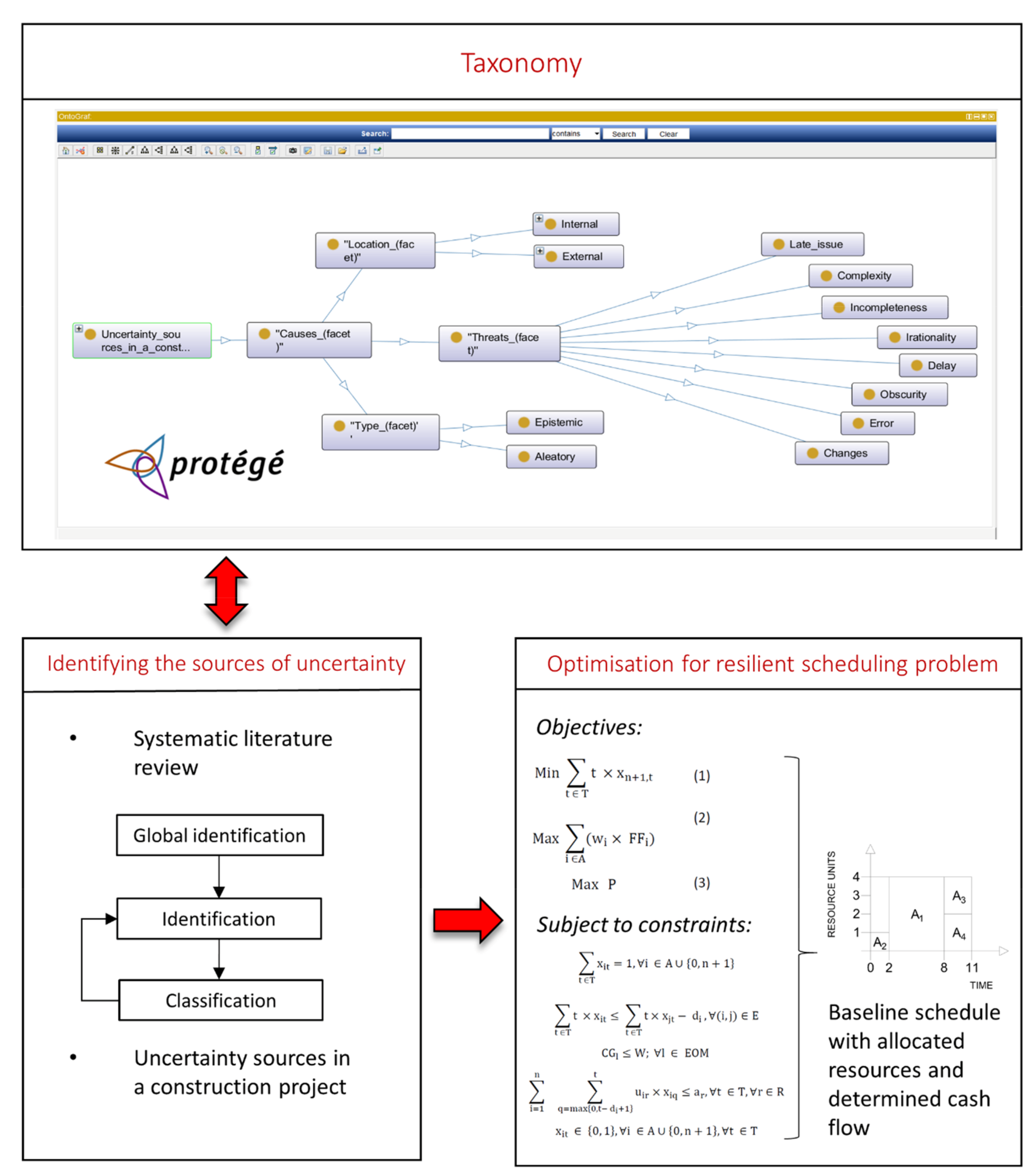
3.1. Solving the Multi-Objective Optimization Problem

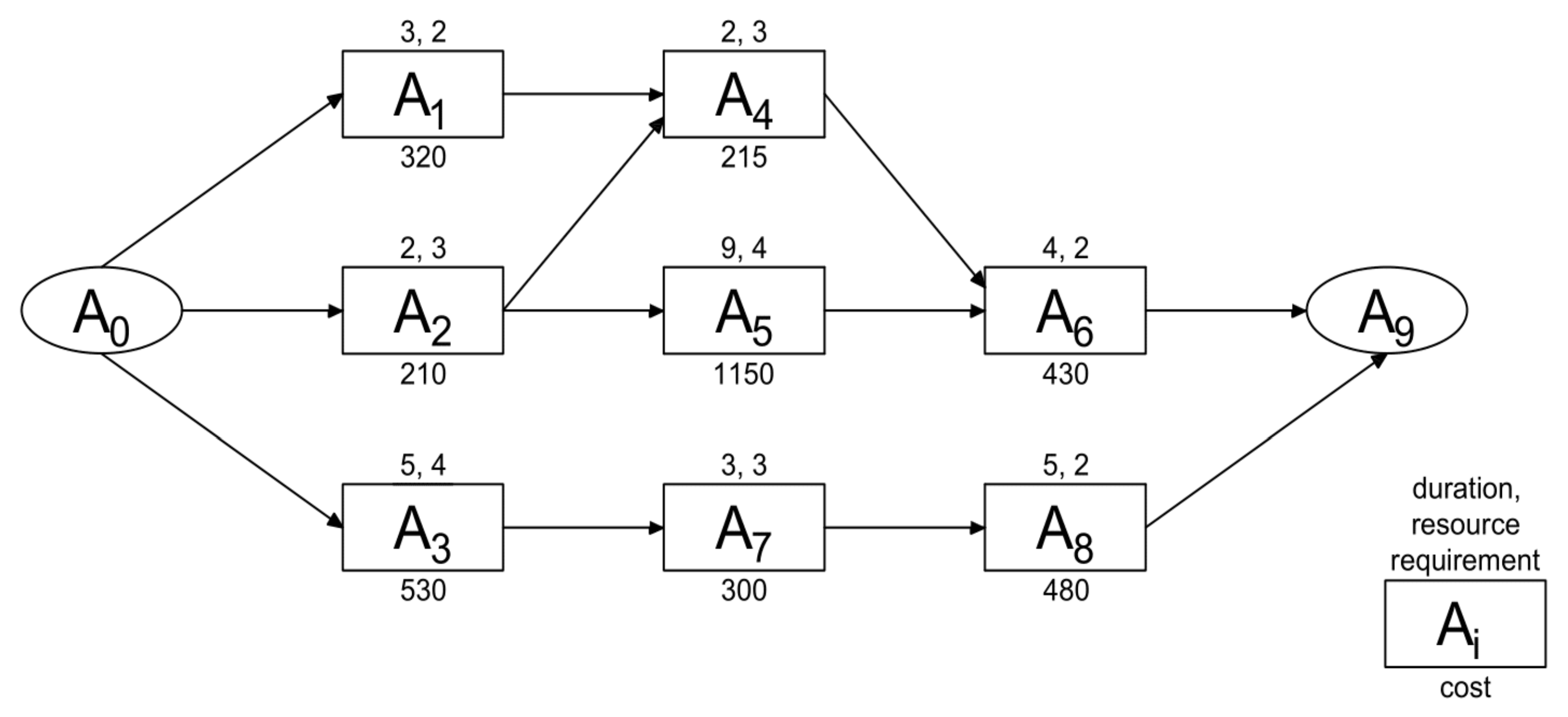
The multi-objective optimization model was applied to the test case adjusted from Reference [30] to provide a detailed description of the solving process for the multi-objective optimization problem on a single problem instance. The activity list for the problem instance is given in

Table 5. Activity list for the problem instance.

Activity Index	Activity Description
${\mathrm{A}}_0$	Dummy start
${\mathrm{A}}_1$	Procurement
${\mathrm{A}}_2$	Field mobilization and site work
${\mathrm{A}}_3$	Landscape equipment mobilization
${\mathrm{A}}_4$	Systems work
${\mathrm{A}}_5$	Structure work
${\mathrm{A}}_6$	Construction finishing operations
${\mathrm{A}}_7$	Landscape earthwork
${\mathrm{A}}_8$	Landscape surfaces
${\mathrm{A}}_9$	Dummy end

. The project network is shown in Figure 3, along with activities’ durations in months, their resource requirement per activity, and activities’ direct costs in thousand of financing units. Only one resource type is required during project execution, of which 7 units are available at any time. Since the model proposed herein requires cash-flow analysis, financial data, and contract terms are provided in

Table 6. Financial data and contract terms for the test instance.

Symbol	Data	Value
OP	Overhead percentage	0.15
MP	Mobilization percentage	0.05
TP	Tax percentage	0.02
MP	Markup percentage	0.20
BP	Bond percentage	0.01
ADV	Advance	0.10
D	Penalty	2
RET	Retainage	0.05
ir	Interest	0.008
h	Surplus	0.005
k	Interest on unused credit	0.002

. All integer values considering financial input are given in thousand of financial units.

In the test case, we assume recognized uncertainty sources as follows:

• Unfavorable weather conditions might interfere with the execution of Activity 2, which is performed on the construction site;
• Architectural innovation involves an element of uncertainty while implementing the Activity 4;
• Change orders in Activity 6 might cause technical difficulty for accomplishing the execution in the estimated time frame.

Having in mind optimization problems with multiple objectives, a single optimal solution cannot always be found in an unambiguous manner. For example, one baseline schedule may provide a shorter makespan, with lower values considering resilience surrogate measure and profit, while another baseline schedule may have a longer duration and significantly higher values of surrogate measure and profit. Therefore, from the mathematical point of view, one optimal solution generally is not guaranteed when solving optimization problems with more than one objective function.

To date, different methods have been introduced to solve the MOO problems. One of them is to combine or weigh different objective functions [67], so the range of solutions can be found as Pareto optimal points. Following this approach, it is hard to obtain a single optimal schedule, since neither of the Pareto solutions can be improved without compromising other objective values [68]. 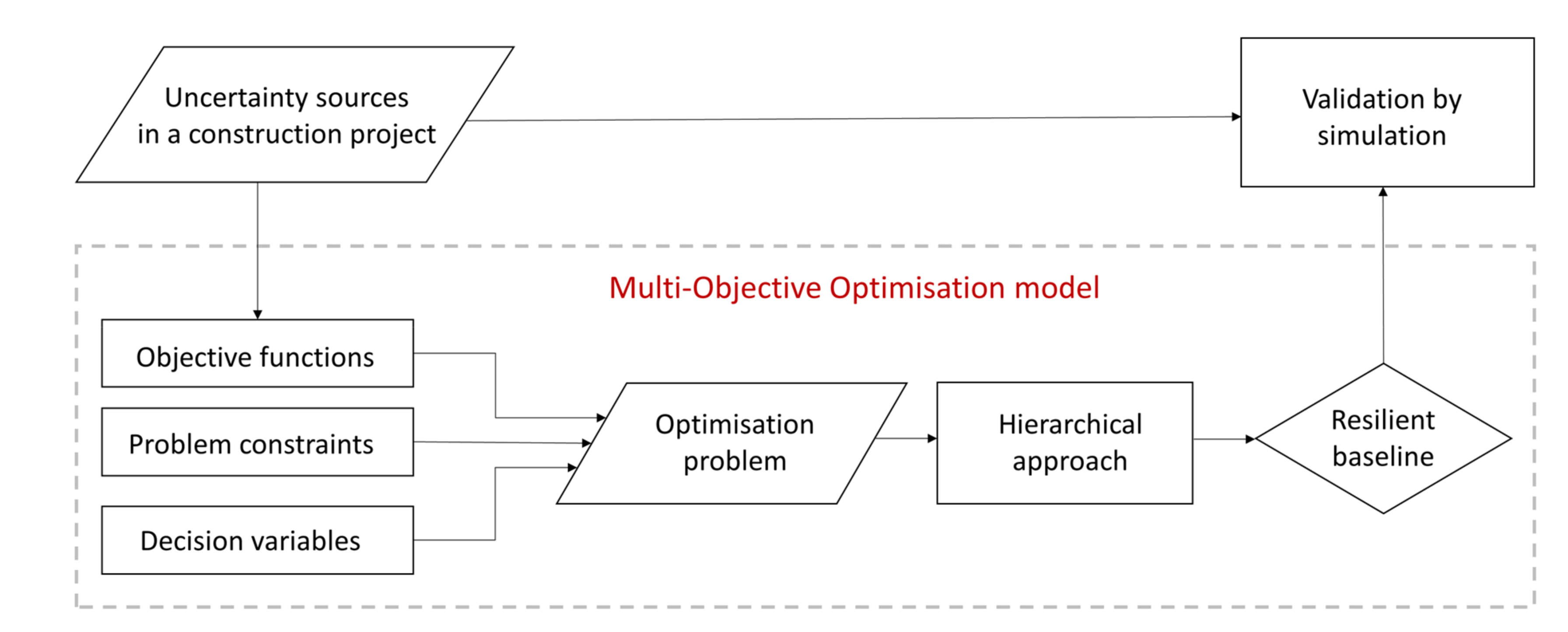As can be seen in Reference [69], although Pareto solutions can be considered broadly comparable, it is not possible to select only one dominant solution. Another problem then arises, as it is not always clear how to combine objective functions with different measurement units. For these reasons, a hierarchical approach was used to proceed with the solving process in the current study.

Since the initial assumption was that the decision-maker’s preferences in obtaining the final solution were known in advance, a hierarchical approach is employed to find a single baseline solution that can be implemented for a construction project. Priorities for all objectives are assigned in decreasing order of importance as follows: timeline minimization, surrogate measure maximization, and profit maximization. This way, project duration is optimized on the uppermost level of the solving process, and the following preference is to find the highest surrogate measure value amongst all solutions that satisfy the first hierarchical objective. At the final step of solving process, a profit value is maximized for the baseline schedule, without causing degradation in earlier objective functions.

The test problem was solved to optimality with an exact algorithm written in the Mathematica programming language. The overall process led to obtaining a single baseline schedule, with a makespan duration of 18 months, SM value of 0.487, and deterministic profit value evaluating to 904.12 thousand of financial units. This way, the stable baseline schedule, which is considered to be resilient under the impact of uncertainty, was produced as a result of the optimization process.

3.2. Validating Resilient Scheduling Process

To validate the resilience of the proposed scheduling process, a probabilistic simulation analysis was conducted for different baseline solutions of the previously presented test problem. Due to the computational complexity of the underlying scheduling problem, the simulation analysis was bounded on two distinctive instances. The first baseline schedule refers to the single makespan instance obtained by solving the MOO test problem as previously described, while the other solution is found when the second and the third objective function were shifted in their hierarchy. For the second case, timeline minimization is still on the highest level of hierarchy in the optimization process; however, the profit maximization is in the second place of importance, and the surrogate measure maximization is at the bottom considering the hierarchical importance of objective functions. This way, the evaluation is made to compare the simulated behavior of two different baseline schedules: both of them have a duration of globally optimal 18 months, but in the first case, the SM value is higher and the baseline profit value is lower compared to SM value and baseline profit value from the second case. Objective function values for both cases are given in

Table 7. Objective function values for two test instances.

Instance	Baseline	Duration	SM	Profit
Case 1	0, 5, 0, 0, 8, 5, 14, 10, 13, 18	18	0.487	904.12
Case 2	0, 0, 3, 0, 5, 5, 14, 7, 10, 18	18	0.353	911.81

, along with the baseline start times for all activities, including dummy start and dummy end. The credit limit was set to 280 thousand of financial units in both cases.

Since the goal of the simulation process is to analyse the project behavior under the impact of uncertainty, some of the activities’ durations in the process of validation are allowed to take stochastic values. For this reason, the duration of activities 2, 4, and 6 in the project network are allowed to take stochastic values. Uncertain activity times are modeled with beta distribution, where shape parameters are set to $\alpha =2$ and $\beta =5$ in order to calculate realised activity durations in the Monte Carlo analysis. Stochastic activity durations in the simulation process are bounded between 0.7 and 2.2 of their estimated length, while the mode of the simulated activities is equal to the planned duration, $d_i$. Considering the simulated direct cost for each activity, it is assumed that the new cost is proportionally related to the realized duration of activity at a ratio, R, which is used to delineate if the cost of activity (C_a) at a simulated duration (T_a) consists mainly of material or equipment and labour. For example, if the cost of activity consists mainly of material, it will have a lower ratio value, R, while higher dependence on equipment and labour will be represented with a higher R-value [70]. In the simulation analysis, R is set to 0.6 for all activities. To calculate activities’ cost C_a at a simulated duration T_a, Equation (14) is employed from the Reference [70]:

$${\mathrm{C}}_{\mathrm{a}}={\mathrm{C}}_{\mathrm{m}}+\frac{({\mathrm{T}}_{\mathrm{a}}-{\mathrm{T}}_{\mathrm{m}})}{{\mathrm{T}}_{\mathrm{m}}}\times \mathrm{R} \times {\mathrm{C}}_{\mathrm{m}} ,{ }_{ }$$

(14)

where C_m represents the original cost of activity at the deterministic duration, T_m.

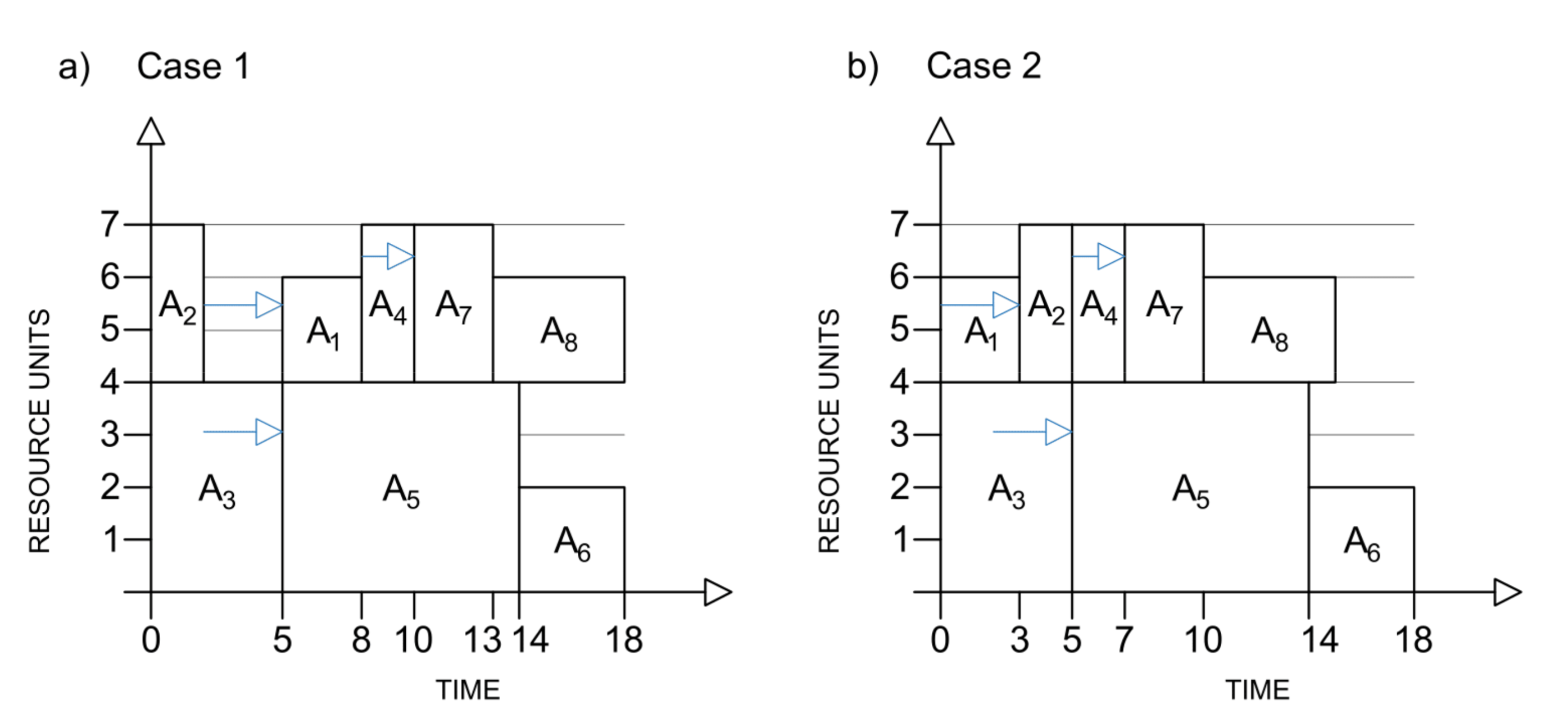
In the simulation analysis, additional resource relations are appended to accompany existing precedence connections between activities, so the baseline resource flow can be preserved throughout the entire simulation process. This way, resource conflicts are avoided through the simulation process where activities’ durations take stochastic values. Additional resource relations are shown for each baseline schedule in Figure 4. Finally, the enhanced Monte Carlo simulation approach, which takes into consideration resource constraints, is taken on 10,000 iterations for each baseline case.

Equilibrium state was examined throughout 6 resilience dimensions: (Eq _i) probability of reaching baseline due date, (Eq _ii) probability of reaching baseline due date multiplied with coefficient 1.1, (Eq _iii) average tardiness amount for the proposed baseline, (Eq _iv) average tardiness amount for activities’ start times, (Eq _v) the percentage of simulations where credit limit was broken, and (Eq _vi) probability of reaching or exceeding the baseline profit. The last equilibrium dimension (Eq _vi) is calculated by considering only those simulations for which credit limit, W, was not broken. From the simulation results, as shown in

Table 8. Simulation results.

Instance	SM Value	Profit	W	Eq i	Eq ii	Eq iii	Eq iv	Eq v	Eq vi
Case 1	0.487	904.12	280	0.3	0.9135	0.66	0.12	1.65%	0.3769
Case 2	0.353	911.81	280	0.2046	0.8249	0.93	0.42	1.73%	0.0978

, it is evident that the first case (single optimal solution from the previous section) generates better results in all equilibrium calculations than the second case, for which profit maximization was considered as a more important objective than maximizing SM value. With an increase in SM value, there is a constant rise in the probability of reaching both strict (Eq _i) and relaxed (Eq _ii) baseline duration, as well as a constant decrease of average project tardiness (Eq _iii), and a decrease of average tardiness for activities’ start times (Eq _iv). Moreover, the percentage of simulations for which the credit limit is broken (Eq _v) is slightly lower in the first case, where the SM value was higher. Finally, the probability of reaching baseline profit or attaining even higher profit values (Eq _vi) is significantly better for the test case with a higher SM value.

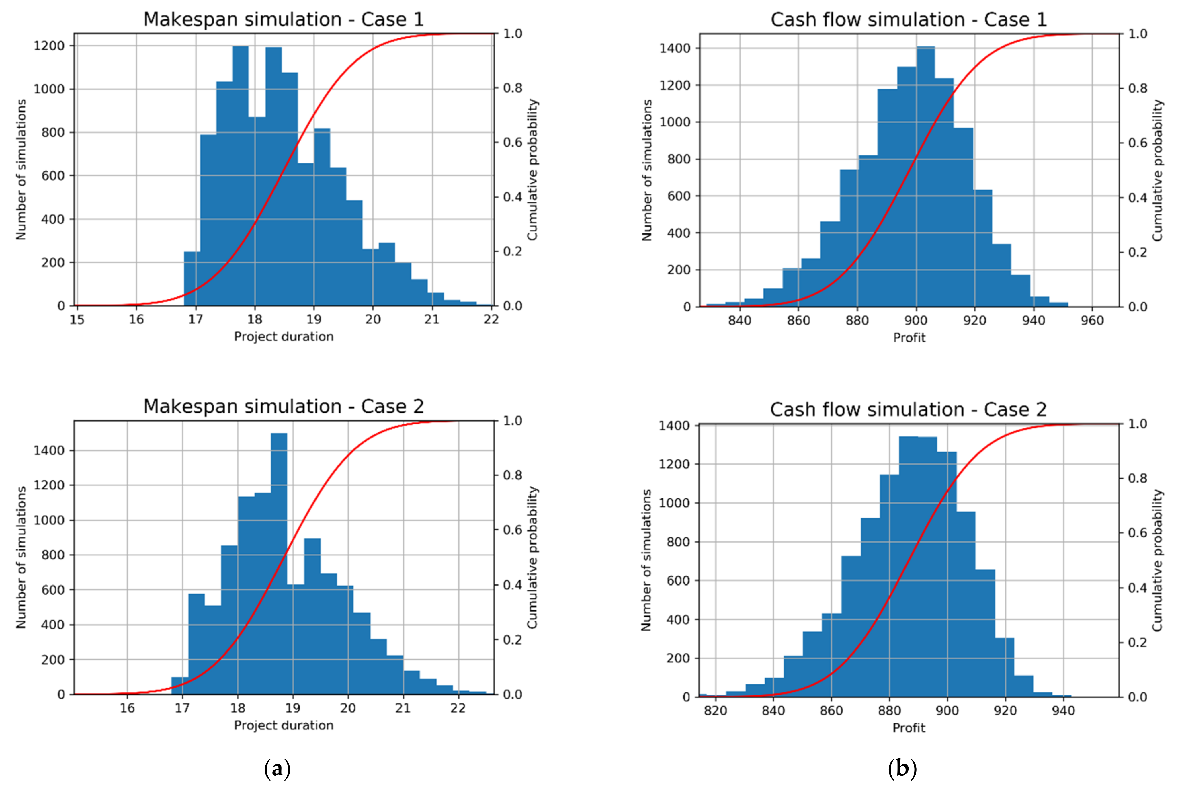
According to the simulation results, the initially suggested approach, where SM value maximization was taken as a more important objective function than maximizing the baseline profit, leads to better results considering the overall resilience of the baseline solution. Validation results indicate a positive correlation between increased SM value and resilience of baseline schedule with allocated resources. As a result of enhanced Monte Carlo analysis, probability distribution charts for makespan duration, considering both cases, are shown in Figure 5a. Probability distribution charts for final profit are shown in Figure 5b.

Since the average deviation of the maximal cash gap is negligible in both baseline cases (average deviation from the negotiated CL was around 0.01% in the simulations where the CL was broken), the probability distribution for profit is shown by considering all simulations, including those where violation of credit limit has occurred. After simulating two different baseline schedules with the Monte Carlo approach, where additional resource relations were appended, it was shown that a schedule with a higher SM value produces a better response to uncertainty.

The results of the equilibrium analysis showed improved performances in all equilibrium dimensions (Eq _i – Eq _vi) when comparing the baseline schedule with higher SM value to another solution in which profit maximization dominated SM improvement. The optimal trade-off between project duration, stability, and profit is obtained for a baseline schedule calculated as a result of the resilient scheduling approach presented in this study. According to validation results, it can be stated that the contractor will benefit from the enhanced resilience of the baseline schedule, since its schedule is improved for the case with the higher SM value. Therefore, this research contributes to the project-management body of knowledge by exploring an approach to develop resilient baseline schedules which will maximize the probability of reaching project goals. With the introduction of the financing aspects in the underlying resilience scheduling problem, the essential issues in construction-management reality are considered. The final output of the MOO problem is given in a form of a baseline schedule which simultaneously minimizes duration of a project, maximizes its resilience, and maximizes final profit from for a contractor. This way, project performances are improved, since the baseline calculations can be accepted with improved confidence levels.

4. Conclusions

In this study, a novel resilience procedure was proposed as a response to prevailing uncertainty in construction projects. In the initial stage of the research, a taxonomy was built to identify uncertainty sources during the life cycle of a project. The formal conceptualization of the domain knowledge, which was modeled in the open-source software Protégé, enables the reuse of information considering the uncertainty in construction projects. The main contribution of the research is the development of the optimization model with three objective functions. This way, a proactive baseline schedule is produced as a result of the optimization process.

Validation results suggest that resilience of a baseline solution improves with SM value maximization. However, the scope of the research was limited to a small project network, so caution must be applied when examining larger problem instances, since the findings might not be unconditionally transferable to a construction projects based on the more complex precedence networks. Although the research has laid the theoretical foundations for resilient scheduling procedure, the study has certain limitations. For example, the resilience framework should be tested on a larger set of project data collected from real construction projects to analyze the systems’ behavior. Moreover, further research might explore different surrogate measures to interpret the resilience capacity of the baseline schedules for various types of construction projects. Finally, the development of new metaheuristic algorithms will enable detailed analysis and validation of the proposed resilience framework on a larger set of problems.

The present research introduces the financing aspect into the process of resilient scheduling, so the comprehensiveness and feasibility of the initial schedule are significantly improved. The advantage of the proposed resilient project planning is enhanced stability of the baseline schedule in comparison with the simulated state of project execution. This leads to more accurate forecasting, so the project-planning calculations are accepted with higher confidence levels.

References

1. Derbe, G.; Li, Y.; Wu, D.; Zhao, Q. Scientometric review of construction project schedule studies: Trends, gaps and potential research areas. J. Civ. Eng. Manag. 2020, 26, 343–363. [Google Scholar] [CrossRef] [Green Version]
2. Faghihi, V.; Nejat, A.; Reinschmidt, K.F.; Kang, J.H. Automation in construction scheduling: A review of the literature. Int. J. Adv. Manuf. Technol. 2015, 81, 1845–1856. [Google Scholar] [CrossRef]
3. Cajzek, R.; Klanšek, U. Cost optimization of project schedules under constrained resources and alternative production processes by mixed-integer nonlinear programming. Eng. Constr. Archit. Manag. 2019, 26, 2474–2508. [Google Scholar] [CrossRef]
4. García-Nieves, J.; Ponz-Tienda, J.; Ospina-Alvarado, A.; Bonilla-Palacios, M. Multipurpose linear programming optimization model for repetitive activities scheduling in construction projects. Autom. Constr. 2019, 105, 102799. [Google Scholar] [CrossRef]
5. Zou, X.; Fang, S.; Huang, Y.; Zhang, L. Mixed-Integer Linear Programming Approach for Scheduling Repetitive Projects with Time-Cost Trade-Off Consideration. J. Comput. Civ. Eng. 2017, 31, 06016003. [Google Scholar] [CrossRef]
6. Klanšek, U. Mixed-Integer Nonlinear Programming Model for Nonlinear Discrete Optimization of Project Schedules under Restricted Costs. J. Constr. Eng. Manag. 2016, 142, 04015088. [Google Scholar] [CrossRef]
7. Liu, Z.; Zhang, Y.; Yu, M.; Zhou, X. Heuristic algorithm for ready-mixed concrete plant scheduling with multiple mixers. Autom. Constr. 2017, 84, 1–13. [Google Scholar] [CrossRef]
8. Sonmez, R.; Iranagh, M.; Uysal, F. Critical Sequence Crashing Heuristic for Resource-Constrained Discrete Time–Cost Trade-Off Problem. J. Constr. Eng. Manag. 2016, 142, 04015090. [Google Scholar] [CrossRef]
9. Li, H.; Xu, Z.; Demeulemeester, E. Scheduling Policies for the Stochastic Resource Leveling Problem. J. Constr. Eng. Manag. 2015, 141, 04014072. [Google Scholar] [CrossRef]
10. Tran, D.; Chou, J.; Luong, D. Multi-objective symbiotic organisms optimization for making time-cost tradeoffs in repetitive project scheduling problem. J. Civ. Eng. Manag. 2019, 25, 322–339. [Google Scholar] [CrossRef] [Green Version]
11. Agdas, D.; Warne, D.; Osio-Norgaard, J.; Masters, F. Utility of Genetic Algorithms for Solving Large-Scale Construction Time-Cost Trade-Off Problems. J. Comput. Civ. Eng. 2018, 32, 04017072. [Google Scholar] [CrossRef] [Green Version]
12. Aminbakhsh, S.; Sonmez, R. Pareto Front Particle Swarm Optimizer for Discrete Time-Cost Trade-Off Problem. J. Comput. Civ. Eng. 2017, 31, 04016040. [Google Scholar] [CrossRef]
13. Sroka, B.; Rosłon, J.; Podolski, M.; Bożejko, W.; Burduk, A.; Wodecki, M. Profit optimization for multi-mode repetitive construction project with cash flows using metaheuristics. Arch. Civ. Mech. Eng. 2021, 21, 1–17. [Google Scholar] [CrossRef]
14. Tao, S.; Wu, C.; Hu, S.; Xu, F. Construction project scheduling under workspace interference. Comput.-Aided Civ. Infrastruct. Eng. 2020, 35, 923–946. [Google Scholar] [CrossRef]
15. Amer, F.; Koh, H.; Golparvar-Fard, M. Automated Methods and Systems for Construction Planning and Scheduling: Critical Review of Three Decades of Research. J. Constr. Eng. Manag. 2021, 147, 03121002. [Google Scholar] [CrossRef]
16. ElMenshawy, M.; Marzouk, M. Automated BIM schedule generation approach for solving time–cost trade-off problems. Eng. Constr. Archit. Manag. 2021. Epub ahead of printing. [Google Scholar]
17. Wang, Z.; Azar, E.R. BIM-based draft schedule generation in reinforced concrete-framed buildings. Constr. Innov. 2019, 19, 280–294. [Google Scholar] [CrossRef]
18. Abbasi, S.; Taghizade, K.; Noorzai, E. BIM-Based Combination of Takt Time and Discrete Event Simulation for Implementing Just in Time in Construction Scheduling under Constraints. J. Constr. Eng. Manag. 2020, 146, 04020143. [Google Scholar] [CrossRef]
19. Dasović, B.; Galić, M.; Klanšek, U. A Survey on Integration of Optimization and Project Management Tools for Sustainable Construction Scheduling. Sustainability 2020, 12, 3405. [Google Scholar] [CrossRef] [Green Version]
20. Nusen, P.; Boonyung, W.; Nusen, S.; Panuwatwanich, K.; Champrasert, P.; Kaewmoracharoen, M. Construction Planning and Scheduling of a Renovation Project Using BIM-Based Multi-Objective Genetic Algorithm. Appl. Sci. 2021, 11, 4716. [Google Scholar] [CrossRef]
21. Xie, L.; Chen, Y.; Chang, R. Scheduling Optimization of Prefabricated Construction Projects by Genetic Algorithm. Appl. Sci. 2021, 11, 5531. [Google Scholar] [CrossRef]
22. Wang, H.; Lin, J.; Zhang, J. Work package-based information modeling for resource-constrained scheduling of construction projects. Autom. Constr. 2020, 109, 102958. [Google Scholar] [CrossRef]
23. Sbiti, M.; Beddiar, K.; Beladjine, D.; Perrault, R.; Mazari, B. Toward BIM and LPS Data Integration for Lean Site Project Management: A State-of-the-Art Review and Recommendations. Buildings 2021, 11, 196. [Google Scholar] [CrossRef]
24. Perminova, O.; Gustafsson, M.; Wikström, K. Defining uncertainty in projects—A new perspective. Int. J. Proj. Manag. 2008, 26, 73–79. [Google Scholar] [CrossRef]
25. Project Management Institute. Construction Extension to the PMBOK Guide; Project Management Institute, Inc.: Newtown Square, PA, USA, 2016; pp. 29–30. [Google Scholar]
26. Ahmad, Z.; Thaheem, M.; Maqsoom, A. Building information modeling as a risk transformer: An evolutionary insight into the project uncertainty. Autom. Constr. 2018, 92, 103–119. [Google Scholar] [CrossRef]
27. Badran, D.; AlZubaidi, R.; Venkatachalam, S. BIM based risk management for design bid build (DBB) design process in the United Arab Emirates: A conceptual framework. Int. J. Syst. Assur. Eng. Manag. 2020, 11, 1339–1361. [Google Scholar] [CrossRef]
28. Xiong, J.; Chen, Y.; Zhou, Z. Resilience analysis for project scheduling with renewable resource constraint and uncertain activity durations. J. Ind. Manag. Optim. 2016, 12, 719–737. [Google Scholar]
29. Yeganeh, F.T.; Zegordi, S.H. A multi-objective optimization approach to project scheduling with resiliency criteria under uncertain activity duration. Ann. Oper. Res. 2020, 285, 161–196. [Google Scholar] [CrossRef]
30. Milat, M.; Knezic, S.; Sedlar, J. A new surrogate measure for resilient approach to construction scheduling. Proc. Comp. Sci. 2021, 181, 468–476. [Google Scholar] [CrossRef]
31. Zhao, M.; Wang, X.; Yu, J.; Xue, L.; Yang, S. A construction schedule robustness measure based on improved prospect theory and the Copula-CRITIC method. Appl. Sci. 2020, 10, 2013. [Google Scholar] [CrossRef] [Green Version]
32. Zhao, M.; Wang, X.; Yu, J.; Bi, L.; Xiao, Y.; Zhang, J. Optimization of Construction Duration and Schedule Robustness Based on Hybrid Grey Wolf Optimizer with Sine Cosine Algorithm. Energies 2020, 13, 2015. [Google Scholar] [CrossRef] [Green Version]
33. Chapman, C.; Ward, S. Project Risk Management: Processes, Techniques and Insights, 2nd ed.; John Wiley & Sons Ltd.: Chichester, UK, 2003; pp. 1–15. [Google Scholar]
34. Zhang, J.; El-Diraby, T.E. Social semantic approach to support communication in AEC. Int. J. Proj. Manag. 2012, 26, 90–104. [Google Scholar] [CrossRef]
35. Elghamrawy, T.; Boukamp, F.; Kim, H.S. Ontology-based, semi-automatic framework for storing and retrieving on-site construction problem information—An RFID-based case study. In Proceedings of the Construction Research Congress 2009: Building a Sustainable Future, Seattle, WA, USA, 5–7 April 2009. [Google Scholar]
36. Tah, J.H.M.; Carr, V. Knowledge-based approach to construction project risk management. J. Comput. Civ. Eng. 2001, 15, 170–177. [Google Scholar] [CrossRef]
37. Tserng, H.P.; Yin, Y.L.S.; Dzeng, R.J.; Wou, B.; Tsai, M.D.; Chen, W.Y. A study of ontology-based risk management framework of construction projects through project life cycle. Autom. Constr. 2009, 18, 994–1008. [Google Scholar] [CrossRef]
38. Ding, L.Y.; Zhong, B.T.; Wu, S.; Luo, H.B. Construction risk knowledge management in BIM using ontology and semantic web technology. Saf. Sci. 2016, 87, 202–213. [Google Scholar] [CrossRef] [Green Version]
39. El-Diraby, T.A.; Lima, C.; Feis, B. Domain taxonomy for construction concepts: Toward a formal ontology for construction knowledge. J. Comput. Civ. Eng. 2005, 19, 394–406. [Google Scholar] [CrossRef]
40. Costa, R.; Lima, C.; Sarraipa, J. Facilitating knowledge sharing and reuse in building and construction domain: An ontology-based approach. J. Intell. Manuf. 2016, 27, 263–282. [Google Scholar] [CrossRef]
41. Niu, J.; Issa, R.R.A. Developing taxonomy for the domain ontology of construction contractual semantics: A case study on the AIA A201 document. Adv. Eng. Inform. 2015, 29, 472–482. [Google Scholar] [CrossRef]
42. Fidan, G.; Dikmen, I.; Tanyer, M.A.; Birgonul, T.M. Ontology for relating risk and vulnerability to cost overrun in international projects. J. Comput. Civ. Eng. 2011, 25, 302–315. [Google Scholar] [CrossRef]
43. Zhang, L.; Issa, R.R.A. Ontology-based partial building information model extraction. J. Comput. Civ. Eng. 2013, 27, 576–584. [Google Scholar] [CrossRef] [Green Version]
44. Baudrit, C.; Taillandier, F.; Tran, T.T.P.; Breysse, D. Uncertainty processing and risk monitoring in construction projects using hierarchical probabilistic relational models. Comp. Aid. Civ. Inf. Eng. 2019, 34, 97–115. [Google Scholar] [CrossRef]
45. Jiang, S.; Wang, N.; Wu, J. Combining BIM and ontology to facilitate intelligent green building evaluation. J. Comput. Civ. Eng. 2018, 32. [Google Scholar] [CrossRef]
46. Xing, X.; Zhong, B.; Luo, H.; Lic, H.; Wu, H. Ontology for safety risk identification in metro construction. Comp. Ind. 2019, 109, 14–30. [Google Scholar] [CrossRef]
47. Zhong, B.; Li, H.; Luo, H.; Zhou, J.; Fang, W.; Xing, X. Ontology-based semantic modeling of knowledge in construction: Classification and identification of hazards implied in images. J. Constr. Eng. Manag. 2020, 146, 04020013. [Google Scholar] [CrossRef]
48. Zhong, B.; Gan, C.; Luo, H.; Xing, X. Ontology-based framework for building environmental monitoring and compliance checking under BIM environment. Build. Environ. 2018, 141, 127–142. [Google Scholar] [CrossRef]
49. Elazouni, A.M.; Metwally, F.G. Finance-Based Scheduling: Tool to Maximize Project Profit Using Improved Genetic Algorithms. J. Constr. Eng. Manag. 2005, 131, 400–412. [Google Scholar] [CrossRef]
50. Fathi, H.; Afshar, A. GA-based multi-objective optimization of finance-based construction project scheduling. KSCE J. Civ. Eng. 2010, 14, 627–638. [Google Scholar] [CrossRef]
51. El-Abbasy, M.; Elazouni, A.; Zayed, T. Finance-based scheduling multi-objective optimization: Benchmarking of evolutionary algorithms. Autom. Constr. 2020, 120, 103392. [Google Scholar] [CrossRef]
52. Damian, D.; Knauss, A.; Zavala, E.; Marco, J.; Franch, X. SACRE: Supporting contextual requirements’ adaptation in modern self-adaptive systems in the presence of uncertainty at runtime. Exp. Syst. Appl. 2018, 98, 166–188. [Google Scholar]
53. Taillandier, F.; Taillandier, P.; Tepeli, E.; Breysse, D.; Mehdizadeh, R.; Khartabil, F. A multi-agent model to manage risks in construction project (SMACC). Autom. Constr. 2015, 58, 1–18. [Google Scholar] [CrossRef]
54. Gündüz, M.; Nielsen, Y.; Özdemir, M. Quantification of Delay Factors Using the Relative Importance Index Method for Construction Projects in Turkey. J. Manag. Eng. 2012, 29, 133–139. [Google Scholar] [CrossRef]
55. Ustinovičius, L. Uncertainty analysis in construction project’s appraisal phase. In Proceedings of the 9th International Conference Modern Building Materials, Structures and Techniques, Vilnius, Lithuania, 16–18 May 2007. [Google Scholar]
56. Ali, Z.; Zhu, F.; Hussain, S. Identification and assessment of uncertainty factors that influence the transaction cost in public sector construction projects in Pakistan. Buildings 2018, 8, 157. [Google Scholar] [CrossRef] [Green Version]
57. Sacco, G.; Tzitzikas, Y. Dynamic Taxonomies and Faceted Search; Springer: Berlin, Germany, 2013. [Google Scholar]
58. Ranganathan, S.R. The Colon Classification; Rutgers University Press: New Brunswick, ME, Canada, 1965. [Google Scholar]
59. Rafindadi, A.D.; Mikić, M.; Kovačić, I.; Cekić, Z. Global Perception of Sustainable Construction Project Risks. Procedia–Soc. Behav. Sci. 2014, 119, 456–465. [Google Scholar] [CrossRef] [Green Version]
60. Warmink, J.J.; Janssen, J.A.E.B.; Booij, M.J.; Krol, M.S. Identification and classification of uncertainties in the application of environmental models. Environ. Model. Soft. 2010, 25, 1518–1527. [Google Scholar] [CrossRef]
61. Hazir, O.; Haouari, M.; Erel, E. Robust scheduling and robustness measures for the discrete time/cost trade-off problem. Eur. J. Oper. Res. 2010, 207, 633–643. [Google Scholar] [CrossRef]
62. Zahid, T.; Agha, M.H.; Schmidt, T. Investigation of surrogate measures of robustness for project scheduling problems. Comput. Ind. Eng. 2019, 129, 220–227. [Google Scholar] [CrossRef]
63. Au, T.; Hendrickson, C. Profit Measures for Construction Projects. J. Constr. Eng. Manag. 1986, 112, 273–286. [Google Scholar] [CrossRef]
64. Ahuja, H. Construction Performance Control by Networks; Wiley: New York, NY, USA, 1976. [Google Scholar]
65. Al-Shihabi, S.; AlDurgam, M. A max-min ant system for the finance-based scheduling problem. Comput. Ind. Eng. 2017, 110, 264–276. [Google Scholar] [CrossRef]
66. Hendrickson, C. Project Management for Construction: Fundamental Concepts for Owners, Engineers, Architects and Builders. Available online: https://www.cmu.edu/cee/projects/PMbook/ (accessed on 18 May 2021).
67. Demeulemeester, E.; Herroelen, W. Project Scheduling; Kluwer Academic Publishers: New York, NY, USA, 2002; p. 67. [Google Scholar]
68. Hapke, M.; Jaszkiewicz, A.; Słowiński, R. Interactive analysis of multiple-criteria project scheduling problems. Eur. J. Oper. Res. 1998, 107, 315–324. [Google Scholar] [CrossRef]
69. Chaturvedi, S.; Rajasekar, E.; Natarajan, S. Multi-objective Building Design Optimization under Operational Uncertainties Using the NSGA II Algorithm. Buildings 2020, 10, 88. [Google Scholar] [CrossRef]
70. Al-Sadek, O.; Carmichael, D. On simulation in planning networks. Civ. Eng. Syst. 1992, 9, 59–68. [Google Scholar] [CrossRef]
Figure 1. Algorithm for the resilience approach to manage uncertainty.
Applsci 11 06493 g001
Figure 2. Layout of the proposed resilience procedure for uncertainty management in construction projects.
Applsci 11 06493 g002
Figure 3. The network of a test problem instance.
Applsci 11 06493 g003
Figure 4. Baseline schedules with additional resource constraints for (a) Case 1 with the highest SM value and lower profit than in Case 2, and (b) Case 2 with the highest profit and lower SM value than in Case 1.
Applsci 11 06493 g004
Figure 5. Simulation results: (a) total project duration (months); (b) total project profit for all iterations in simulation, CL may be broken (thousand of financing units).
Applsci 11 06493 g005