Bearing Severity Fault Evaluation Using Contour Maps—Case Study

Abstract

Increasing industrial competitiveness has led to an increased global interest in condition monitoring. In this sector, rotating machinery plays an important role, where the bearing is one of the most critical components. Many vibration-based signal treatments are already being used to identify features associated with bearing faults. The information embedded in such features are employed in the construction of health indicators, which allow for evaluation of the current operating status of the machine. In this work, the use of contour maps to represent the diagnosis map of a bearing, used as a health map, is presented for the first time. The results show that the proposed method is promising, allowing for the satisfactory detection and evaluation of the severity of bearing damage. In this initial stage of the research, our results suggest that this method can improve the classification of bearing faults and, therefore, optimise maintenance processes.

1. Introduction

At present, the continuous and correct operation of machines is crucial in an increasingly competitive industrial sector. Thus, fault monitoring and diagnosis are some of the most critical aspects of equipment design and maintenance [1]. According to Shao et al. [2] and Behzad et al. [3], rotating machinery plays an important role in modern industries, with the bearing being one of the most critical components. Nguyen et al. [4] stated that this component is responsible for up to 50% of failures in rotating machinery, while Graney and Starry [5] argued that only 10% of bearings reach the end of their useful life.

This has created the need for Condition Monitoring (CM) systems, which ensure the safety and reliability of the operation of the equipment [1,6,7,8]. CM focuses on the study of the behaviour of the machine, by applying non-intrusive techniques such as “Vibration Analysis,” given its early appearance [9,10]. In this way, CM identifies and characterises anomalous changes in operations due to the degradation of the mechanism [11]. There are three key stages to ensure the highest efficiency in fault diagnoses, such as log capture, data processing and information management [12,13]. On the other hand, the ISO 13373 [14,15] standard provides a detailed guide of the parameters to be used at each stage.

It should be noted that this first stage has been treated in a previous study [16], where the authors presented a low-cost, high-frequency data acquisition system based on a Raspberry Pi, which allows for the application of CM to bearings in rotating machinery. Continuing this research, this work focuses on the second stage, in which data processing methods are studied. The ISO 13373-2 [15] standard defines this stage as the group of activities that, based on the processing of the acquired signals, allows for the identification of characteristics of the mechanism under study (in this case, bearings).

In recent years, different methods have been proposed for the extraction of information from vibration signals, related to the state of bearings. One of the most powerful tools used at present is artificial intelligence [1,17], in which the extraction of characteristics plays an important role in the diagnosis. In this way, feature classifiers such as Support Vector Machine (SVM) algorithms [18,19], deep learning techniques [20,21] or both [22] have taken centre stage. Zhang et al. [6] proposed a model based on deep learning, which is capable of adapting to industrial environments, where changes in load and noise are the main drawback. On the other hand, Liu et al. [23] presented an unsupervised learning method with better accuracy in the classification of fault characteristics, compared to existing machine learning and deep learning methods. In addition, traditional data processing techniques include diagnostic methods based on different techniques; for example, an autoregressive model has been proposed for filtering signals [24] or the decomposition of the signal for the extraction of characteristics using Empirical Mode Decomposition [25,26] and Ensemble Empirical Mode Decomposition [27,28] has been performed. Moreover, Feng et al. [29] and Brusa et al. [30] used signal demodulation by envelope analysis to extract characteristic fault frequencies. On the other hand, some authors have used tools such as spectrograms [31,32], kurtograms [33] or bispectra [33,34] to detect the presence of transient events in a signal.

There are other concepts of surface analysis, such as contour maps (isolines), which have been widely used in various fields to represent the study environment, instead of specific data. In medicine [35,36], contour maps are used for the segmentation of two-dimensional images, which allows for the elimination of blurring effects and improves the identification of regions corresponding to the study objects. In topography [37,38,39], contour maps are used to indicate elevations and features of geographical accidents. In finance [40], contour maps are used to represent the estimation error and global minimum risk. In manufacturing [41], contour maps are used as a graphical tool to estimate the machining error or kinematic error. In meteorology [42], contour maps are used to represent weather conditions. In navigation [43], contour maps are used to represent risk regions and safe navigation routes. In additive manufacturing [44,45,46,47], contour maps are used to describe the details of the model to be 3D printed.

The literature on the application of contour maps to condition monitoring is very scarce. Li and Liu [48] proposed the use of Iso-Map in wireless sensor networks to reduce energy costs. Meng et al. [49] used contour maps to monitor and diagnose sensor networks to visualise the network in the spatial and temporal domains, as well as to detect sensors that are failing; however, no publication has been found that applies contour maps to bearing failure level classification.

On the other hand, the existing fault classification methods can be divided into indirect ones, which require the implementation of artificial intelligence [13,50], and direct methods [13,50]. The use of contour maps to graph and predict the level of failure is a direct method that does not require a priori learning. However, unlike other direct methods, it gives a continuous idea of all the failure states of the bearing from which its failure map or footprint has been obtained. Furthermore, for each record to be classified, there will be a multitude of points on each map associated with the frequencies studied (i.e., fundamentals and harmonics). Thus, the proposed method will be a robust tool for fault diagnosis.

The present work presents the first steps to assess the possible use of contour maps, based on Envelope Analysis, to generate a bearing degradation map. This map will allow us to classify the failure status of a bearing, based on its footprint or failure map. As it is represented in two dimensions, it offers a broader view of the relationship between the frequency of failure, level of failure and amplitude associated with each fault level. For this, a work methodology was developed and implemented in MATLAB^®, which was applied to real measurements. The results suggest that this methodology can help in the prediction of bearing failures.

The document is organised as follows: Section 2 analyses the steps and criteria considered in the construction of contour maps. Section 3 reviews the diagnostic results of different registries. Finally, Section 4 presents the conclusions of this study and analyses directions for future work.

2. Method

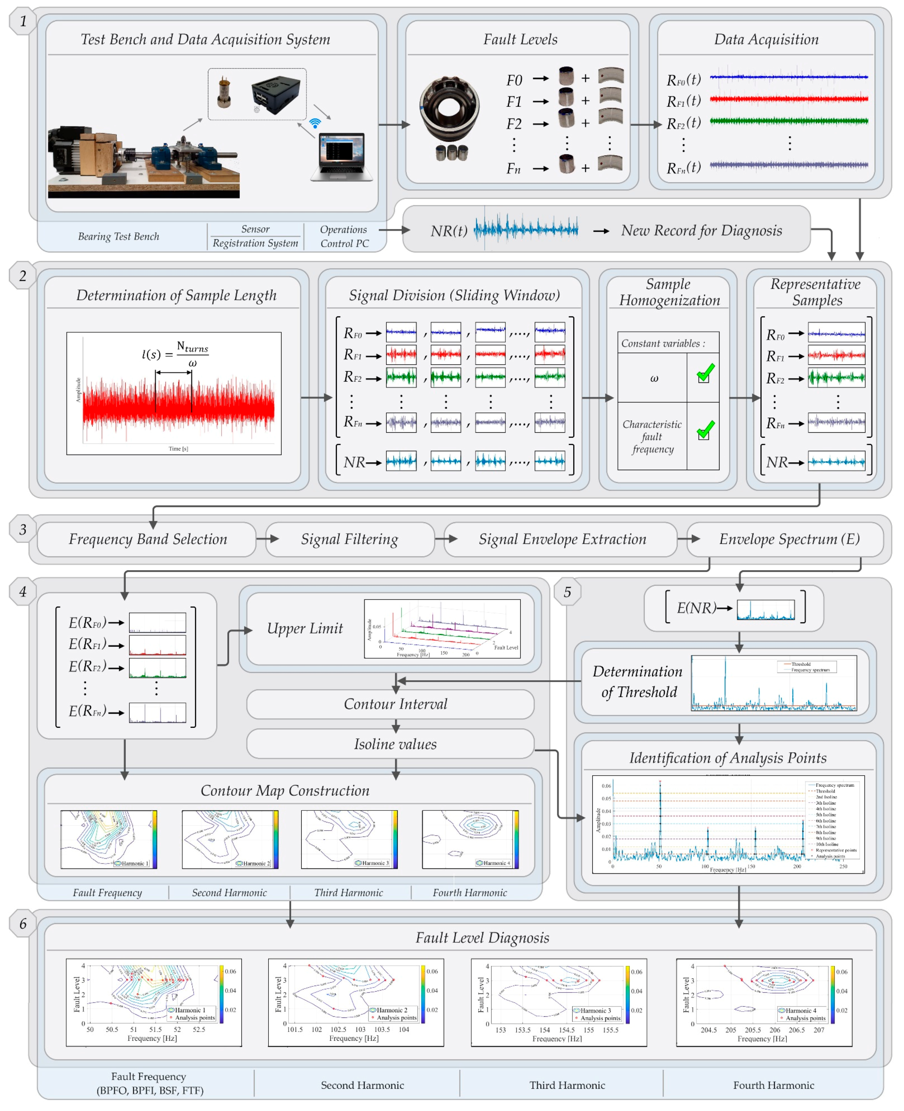
The main objective of this method is to build health maps for bearings, which allow for the efficient and accurate assessment of the severity of a fault. For this purpose, the variation of vibration amplitudes is characterised (by means of envelope analysis) for each characteristic frequency of a bearing (i.e., fundamental frequencies) and harmonics. In other words, in this study, bearing health maps are constructed, considering the effect caused by each type of failure (fundamental frequencies) on the power content of the signal. For this, the use of Contour Maps is proposed, which allows us to compact the information and better understand the footprint generated in fault evolution. The main phases of this method are presented below:

• The sensing of the equipment under analysis and acquisition of vibration records for different fault levels (F0, F1, …, Fn), marking the life history of the bearing. We obtained a record for each fault level in the time domain, $R_{F0}\left(t\right),\dots , R_{Fn}\left(t\right)$. This study presents the creation of the life history of a bearing located on a test bench [16], considering four failure levels (n = 4) and the normal state, as described in Section 2.2.
• The extraction of representative samples of records that were taken in Phase 1 (Section 2.3).
  • The determination of the sample time length, $l\left(s\right)=\frac{number of turns}{w\left(rps\right)}$.
  • The division of the signal into intervals by means of a sliding window, with the sample length calculated in (2.a).
  • The identification of intervals with constant angular velocity for each fault level.
  • The selection, among the time intervals identified in (2.c), of the intervals with both constant angular velocity and fault frequency (BPFO, BPFI, BSF, FTF). The first interval that accomplishes these conditions is the selected one. This procedure will allow for consideration of the possible slippage between the contact of rolling elements and the inner and outer races.
• A pre-processing stage, which will be applied to each fault level’s selected time interval, (Section 2.4).
  • Frequency band selection in the presence of transient events associated with bearing fault modes.
  • Signal filtering using the selected frequency band, obtaining a time-domain filtered signal (2.a).
  • Signal envelope extraction (time domain), from the signal of (3.b).
  • Envelope Spectrum (frequency domain), from the signal (3.c).
• The processing and construction of the Contour map of the Envelope Spectrum, representing the fault level, frequency and amplitude (associated to 3d).
  • Consideration of the threshold value calculated with the spectrum to be diagnosed 5.a, $E\left(NR\right)$, as described in Section 2.5.1.
  • The identification of the upper limit associated with the highest amplitude frequency of the envelope spectrum used in the construction of the contour map, $E\left(R_{F0}\right)$, $E\left(R_{F1}\right)$,…, $E\left(R_{Fn}\right)$, as described in Section 2.5.2.
  • Contour interval estimation (Section 2.5.3).
  • The calculation of the values of the isolines (Section 2.5.4).
• The treatment of the new record, $NR\left(t\right)$, or record to be diagnosed (the new record will also be subjected to the criteria stipulated in Phases 2 and 3).
  • The determination of the threshold value or isoline of the lowest value (Section 2.5.1).
  • The identification of the analysis points or points of intersection between the amplitudes of the spectrum to be diagnosed and the isoline values (Section 2.6).
• Diagnosis of the failure level of the new record ($NR$), using the contour map created in Phase 4 of the proposed method.

The abbreviations indicated in the description of the method and variables used in the construction of the contour maps and the bearing diagnosis are expressed in the form of nomenclature in

Table 1. The nomenclature used in the construction of contour maps and bearing diagnostics.

Nomenclature	Description
$Fn$	Fault levels
$Rn$	Shaft rotational speed
$R_{Fn}$	Record for each fault level in the time domain
$E\left(R_{Fn}\right)$	Envelope spectrum of the record of each fault level
$l$	Sample time length in seconds
$N_{turns}$	Number of shaft turns
$w$	Constant angular velocity
$NR$	New record to be diagnosed in the time domain
$E\left(NR\right)$	Envelope spectrum of the record to be diagnosed
$F_r$	Frequency of shaft rotation
$N_b$	Number of rolling elements of the bearing
$S_{low}$	Lower limit of the analysis section
$S_{up}$	Upper limit of the analysis section
X	Sample or data set under analysis
N	Length of the sample under analysis
$R_a$	Range of analysis
$N_{int}$	Number of intervals
$X_i$	Mean value of the amplitudes of the analysed sample
I	Width between intervals
$f_i$	Number of components in each interval
$\overline{x}$	Arithmetic mean of the distribution of amplitudes
X2	Significant amplitude data set
$N_2$	Length of the significant amplitude data set
$N_{iso}$	Number of isolines
$k$	Multiple of the spacing value
$BPFO$	Ball Pass Frequency Outer
$BPFI$	Ball Pass Frequency Inner
$BSF$	Ball Spin Frequency
$FTF$	Fundamental Train Frequency

.

The method described above, based on six main phases, is detailed in Figure 1.

The literature has emphasised the importance of identifying frequency bands of a signal, with the presence of transient events associated with the bearing condition. However, in this study, we intended to analyse the behaviour of the footprint of the evolution of a fault, according to the frequency bands proposed in [16]. Therefore, various contour maps are made for the selected frequency bands. For each frequency band, several contour maps will be built around selected frequencies. In each contour map, the main fault frequencies and their most representative harmonics are displayed, with a range of ±1 Hz. In this way, several contour maps are used to classify future measurements of the study machine and, thus, identify the state of fault that the bearing is in. Contour maps that present a unique relationship between frequency, amplitude and failure will allow for better future classification of the condition of this bearing throughout its useful life.

The following sections provide more clarification about key parts of the described method.

2.1. Contour Map

The concept of a “Contour Map” is simple and well-known. Contour maps are graphs that, although being two-dimensional visually, they actually represent three dimensions, by including contour lines (or isolines) [39]. In this way, a contour map compactly represents a function of space using a small set of isolines. Morse [51] defined isolines as lines of intersection between the points of a given surface and a family of parallel planes. 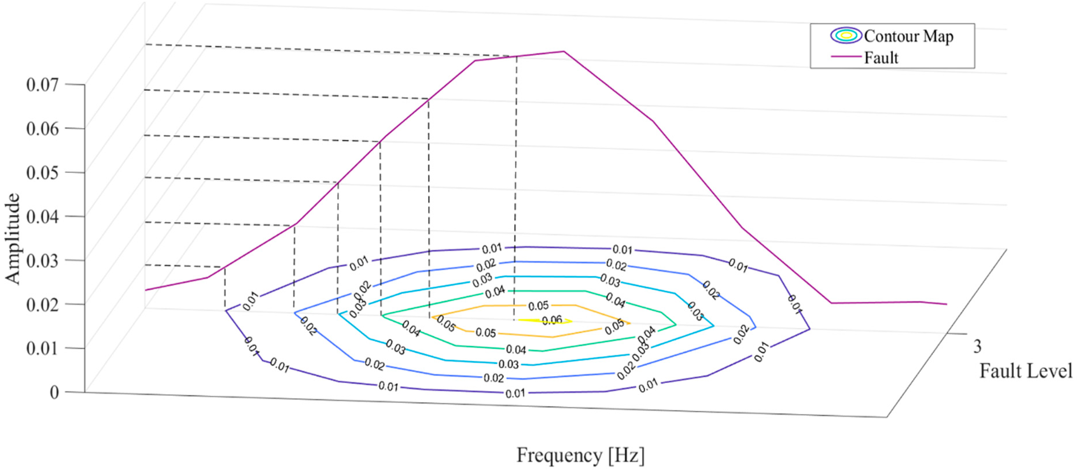Thus, each isoline classifies and separates the points of the underlying space, joining the points with a constant and equally spaced contour value [43,52], as shown in Figure 2. In this figure, the contour map is shown in two dimensions, where it is indicated that each isoline is associated with a height (frequency amplitude, in this case). These heights, represented by different colours on the contour map, corresponding to the real heights of the surfaces formed for each fault level. The curve corresponding to a specific failure level is shown in purple, as an example.

As previously indicated, this research is based on contour maps, which are generated to describe the evolution of the failure of a bearing component, with respect to its fundamental frequency. Following the recommendations for the construction of contour maps, the spacing value (contour interval) between isolines will remain constant and, in this case, correspond to values of amplitude in the frequency of the vibration. The range of values is selected according to a series of criteria, which are detailed in the following sections.

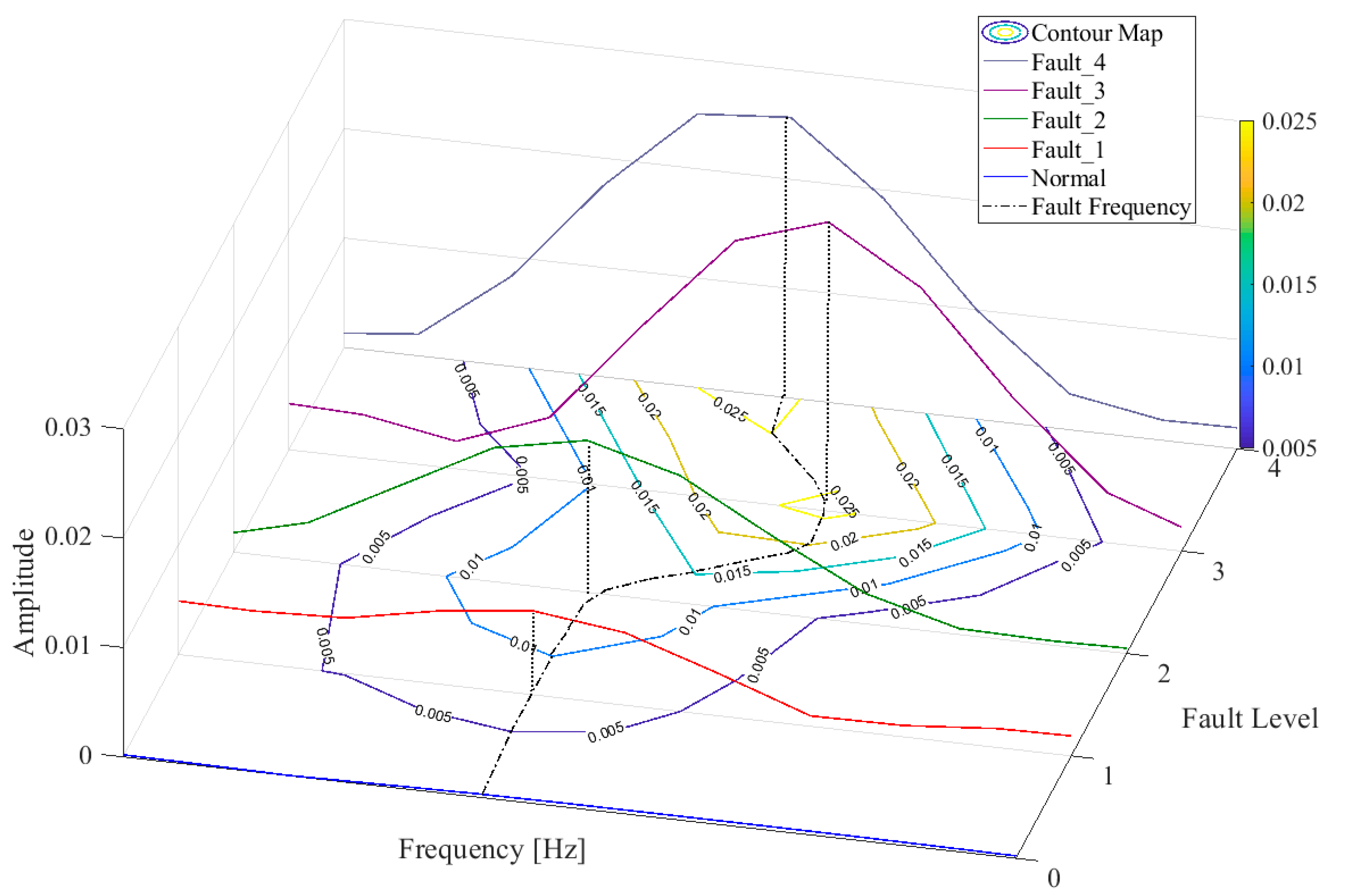
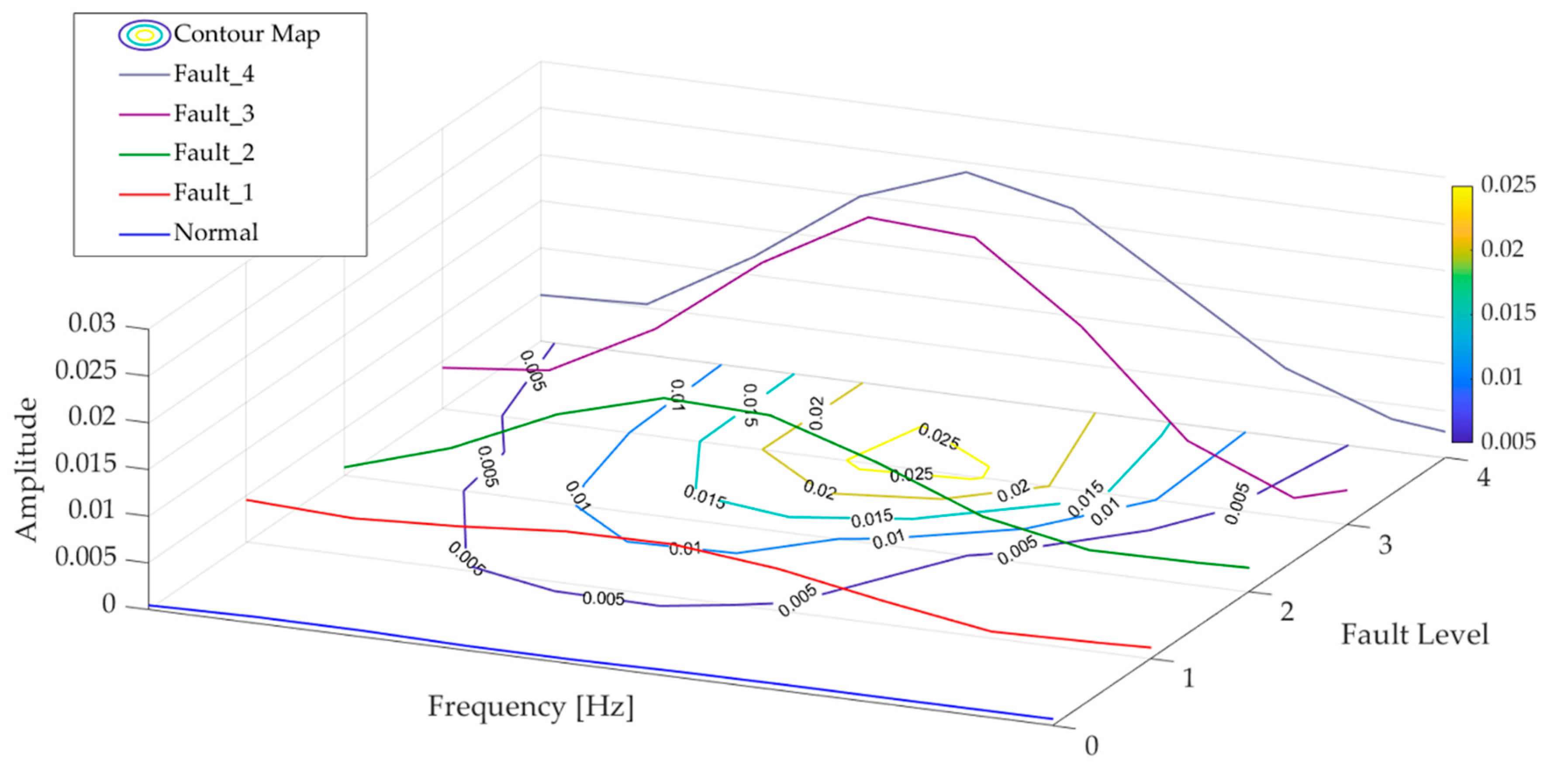
As an example, in Figure 3, the evolution of the amplitude of a fundamental frequency in the presence of a fault is observed, where the set of values that characterise the analysis amplitudes are in a range from 0.005 to 0.025, equally spaced to a contour interval equal to 0.005. The contour map is, therefore, equivalent to having the evolution curves of a fault frequency in a compact form.

It should be noted that the signal associated with the normal operating state has an amplitude with a value other than zero. However, its magnitude is negligible, compared to the amplitude of a severe fault. For this reason, Figure 3 shows the closeness between the normal state signal and the zero-value axis.

Table 2. The amplitude of the spectra is presented in Figure 3.

Fault Level	Mean Amplitude	STD	STD (% Mean Value)
0	0.0004871	0.000107709	22.11
1	0.005675	0.00185744	32.72
2	0.01266	0.00448274	35.41
3	0.0263	0.00932127	35.44
4	0.02395	0.00780833	32.60

presents the value of the amplitudes of the evolution of a fault frequency shown in Figure 3.

2.2. Experimental Data

As indicated in the proposed method, contour maps are constructed based on the fault evolution of a bearing component, relating frequency, amplitude and fault level in each contour map. From a theoretical point of view, the more levels of failure included, the greater the precision of the contour map or fault map. From a practical point of view, it is not always easy to gradually increase the level of failure in the element of study. On the other hand, it is also important to have a record of optimal operating conditions of the bearing to be analysed. This allows for the transition between a normal operating state and incipient failure to be considered.

2.2.1. Experiment Details

The study [16] on which this work is based addressed the development of low-cost recording equipment with a sampling frequency of up to 45 kHz in three of its channels, applicable to bearing condition monitoring. In this previous investigation, its characteristics were validated by capturing records of simulated failures in the test bench bearing.

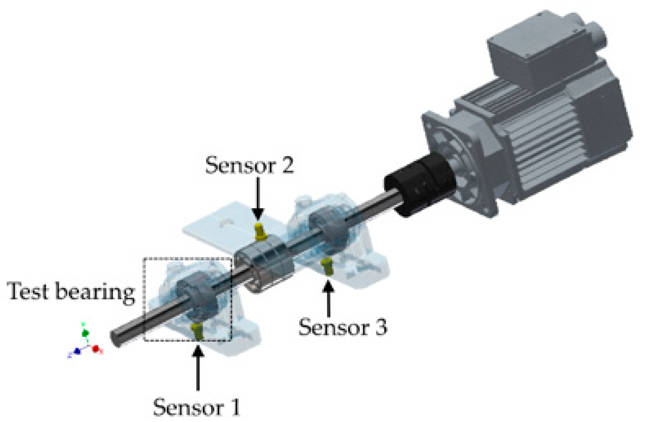
This test bench contained two supports with double-row spherical roller bearings 22205E1KC3 (Sensor 1 and Sensor 3), one of which corresponded to the test bearing, as shown in Figure 4. Their Ball Pass Frequency Inner (BPFI), Ball Pass Frequency Outer (BPFO), Ball Spin Frequency (BSF), and Fundamental Train Frequency (FTF), evaluated at different angular speeds (and turning frequency, F_r), are presented in

Table 3. Fundamental frequencies of the 22205E1KC3 bearing (Sensors 1 and 3) under different regimes [16].

22205E1KC3	Frequency	Regime			Units
		200	350	500	rpm
BPFO	6.1852 × Fr	20.62	36.08	51.54	Hz
BPFI	8.8148 × Fr	29.38	51.42	73.46	Hz
BSF	5.4030 × Fr	18.01	31.52	45.03	Hz
FTF	0.4123 × Fr	1.37	2.41	3.44	Hz

.

In addition, three 6304-2R (Sensor 2) ball bearings were continuously positioned between the housings. The characteristic failure frequencies are presented in

Table 4. Fundamental frequencies of the 6304-2R bearing (Sensor 2) under different regimes [16].

6304-2R	Frequency	Regime			Units
		200	350	500	rpm
BPFO	2.5783 × Fr	8.59	15.04	21.49	Hz
BPFI	4.4398 × Fr	14.80	25.90	37.00	Hz
BSF	1.7590 × Fr	5.86	10.26	14.66	Hz
FTF	0.3687 × Fr	1.23	2.15	3.07	Hz

. These allow for exerting a vertical load on the shaft. Each support bearing and load zone bearings have a piezo-ceramic accelerometer, positioned orthogonal to the axis (Figure 4).

2.2.2. Design of Experiment (DoE)

The DoE was based on the development of a combined outer race (OR) and three rolling elements (RE) failures in the test bearing. For this, a “Factorial 5 × 3” design was considered, to study the influence of five fault levels (F0, F1, F2, F3 and F4) on ORRE, under three operating regimes (200, 350 and 500 rpm).

Table 5. Factors and levels considered in the design of the experiment.

Study Factor		Levels					Units
		F0	F1	F2	F3	F4
RE	Area	0	11.05	11.57	11.7	13	mm2
	Depth	0	0.006	0.014	0.019	0.027	mm
OR	Area	0	25.874	28.928	31.983	33.241	mm2
	Depth	0	0.007	0.013	0.02	0.028	mm
Control Factor		Levels					Units
		R1		R2	R3
Regime		200		350	500		rpm

describes the factors and levels considered in the test.

The depth of the fault is expressed as the absolute magnitude of the difference between the geometry of the normal state and the induced fault. The development of the flaws was generated by milling the surface of each component, their quantification was carried out using a DML IP54 micrometre.

The ISO 13373-1 [14] standard indicates that the load is one of the most influential factors in vibration; therefore, the fault generated in OR must be positioned in the load zone of its support. As indicated by Soto-Ocampo et al. [16], a threaded tightening tower was used in this experiment, which allows for a vertical load of 1.4 kN to be applied.

The type of lubricant used in the bearing is the one recommended on the official Schaeffler website (ISO VG 220) for the operating conditions. Considering the influence of a correct lubricant film on the friction level and heat dissipation between the bearing components, a protocol was executed prior to the start of the record capture at each failure level. This ensures correct lubrication and maintains the same working conditions at each record capture. This protocol considered the change the lubricant at each fault level generated and the preheating of the bearing, for which two stages of operation were carried out, starting with 10 min of operation at a rotational speed of 200 rpm and then continuing with 10 min of work at a rotational speed of 500 rpm. After these operations, the engine turns to the speed test (200 rpm). Each event was repeated three times, where the most representative replica was obtained through the geometric mean of the correlation, covariance and coherence estimators. These estimators analyse the relationship between replicas in the frequency domain. The most representative replicas will also be used in this work.

The records were acquired with a sampling frequency of 45 kHz in three of its channels, for 45 s. These, in turn, were resampled at 40 kHz to guarantee a constant sample rate throughout the record.

2.3. Angular Speed Influence

During this investigation, we observed that the turning speed is also an important parameter to consider in the representation of contour maps. Fernandez-Francos et al. [53] emphasised the importance of keeping the rotational speed constant when capturing logs. Thus, by analysing vibrations at a constant angular velocity, repetitive impacts can be identified through the characteristic frequencies of the bearing. This criterion was applied in the analysis by means of contour maps, to eliminate frequency lags and variations in the impact force, as shown in Figure 5.

Figure 6 represents the segment of the contour map associated with a fault, built with the records used in Figure 5. In this case, the entire length of the record (45 s) was used. Obviously, the registers have a variable speed of rotation in each second. Thus, the frequency represented in the contour map will be associated with the predominant turning speed which, as observed, was not equivalent between fault levels. Added to this was the large number of points used to construct the contour map, causing a loss of information between fault levels.

For the identification of the segments at a constant speed, we carried out a scan of the signal of each record (time domain), which forms the contour map and the record to be analysed. Subsequently, the rotation frequency was identified in the envelope spectrum. Given that different rotation speeds are handled in this work, drawbacks were observed in establishing the same analysis section for all rotation regimes. For this reason, we proposed to determine the sweep section of the signal, based on the number of turns of the shaft. Observing that, regardless of the turning speed, for a number of 17.5 turns, the same turning frequency can be properly identified in each register.

Table 6. Representation of the section of the register used in each rotational speed, associated with 17.5 turns.

Shaft Turns	Regime [rpm]	Register Section [s]
17.5	200	5.25
	350	3
	500	2.1

presents the section of the register used in each rotation regime.

Despite identifying register sections at a constant speed, it was necessary to consider the slip at the contact between the rolling elements and the races, which occurs during the operation of a bearing. This creates uncertainty in the identification of fault frequencies. Smith and Randal [54] considered a variation of the calculation of the frequencies between 1% or 2%, from which the following hypothesis can be established:

The maximum amplitude-frequency close to the theoretical fault frequency, in a range of ± 1% of the theoretical frequency, corresponds to the actual fault frequency.

From this, once the constant velocity sections have been identified—and considering the previously described hypothesis—the sections of each record were identified, where the actual failure frequencies coincided.

2.4. Signal Pre-Processing

In the pre-processing of the data, the oscillatory fundamentals of the bearing were considered, using an analysis technique that allows for the identification of the resonant areas associated with the state of the bearing components. In the construction of contour maps, the maximum amplitude of the spectrum plays a crucial role in the definition of each isoline, as shown in Figure 2. Raviola and Fiori [55] indicated that the passage of a rolling element over a defect generates a transient event that excites the resonance frequencies of the bearing structure (BPFO, BPFI, BSF or FTF). Therefore, the presence of a defect is evident in the amplitude of the signal spectrum, at the defect fundamental frequencies.

This is why there is a need to develop a data processing technique that is capable of extracting relevant failure information from the components of a bearing, as well as filtering the background noise as much as possible. The study prior to this analysis [16] supported the use of the “Envelope Analysis” technique in the pre-processing of data, due to the sensitivity it presented to bearing fault oscillations. Likewise, we proposed the evaluation of the frequency bands proposed in [16] (0.2–1.8 × 10³; 1.8–6.1 × 10³; 6.1–9.2 × 10³; and 9.2–12.8 × 10³ Hz) for filtering the measured signal, as well as the use of the Hilbert transform to determine the envelope of the signal.

2.5. Contour Maps Set-Up

In the construction of the contour maps, a series of criteria were considered to evaluate the bearing failure evolution. In data processing programs such as MATLAB^® (“contour” function), from the data provided (bearing failure evolution records), the limits and the spacing between each isoline are determined by default from the scale of the frequency of greater amplitude, as seen in Figure 2 and Figure 3.

However, sometimes these default estimated values for each isoline do not allow the analysis of records corresponding to a normal state or incipient failure, where the isoline with the lowest amplitude is above the amplitude of the frequency under analysis. This is because the limits and the isoline value are calculated based on the maximum amplitude signal, which is normally associated with a severe bearing failure record. This is why the lower limit of construction of the contour map must be adjusted to the behaviour of the record to be analysed, maintaining the maximum amplitude value of the records that make up the contour map and calculating a spacing value between isoline lines consistent with the record in analysis.

On the other hand, setting the spacing value brings about some inconveniences. If the spacing value is too large, there may be issues in diagnosing normal status and early failure records. Likewise, if the spacing value is very small, the computational expense will increase and a large amount of isolines will make the interpretation of the data difficult, as indicated in Figure 7.

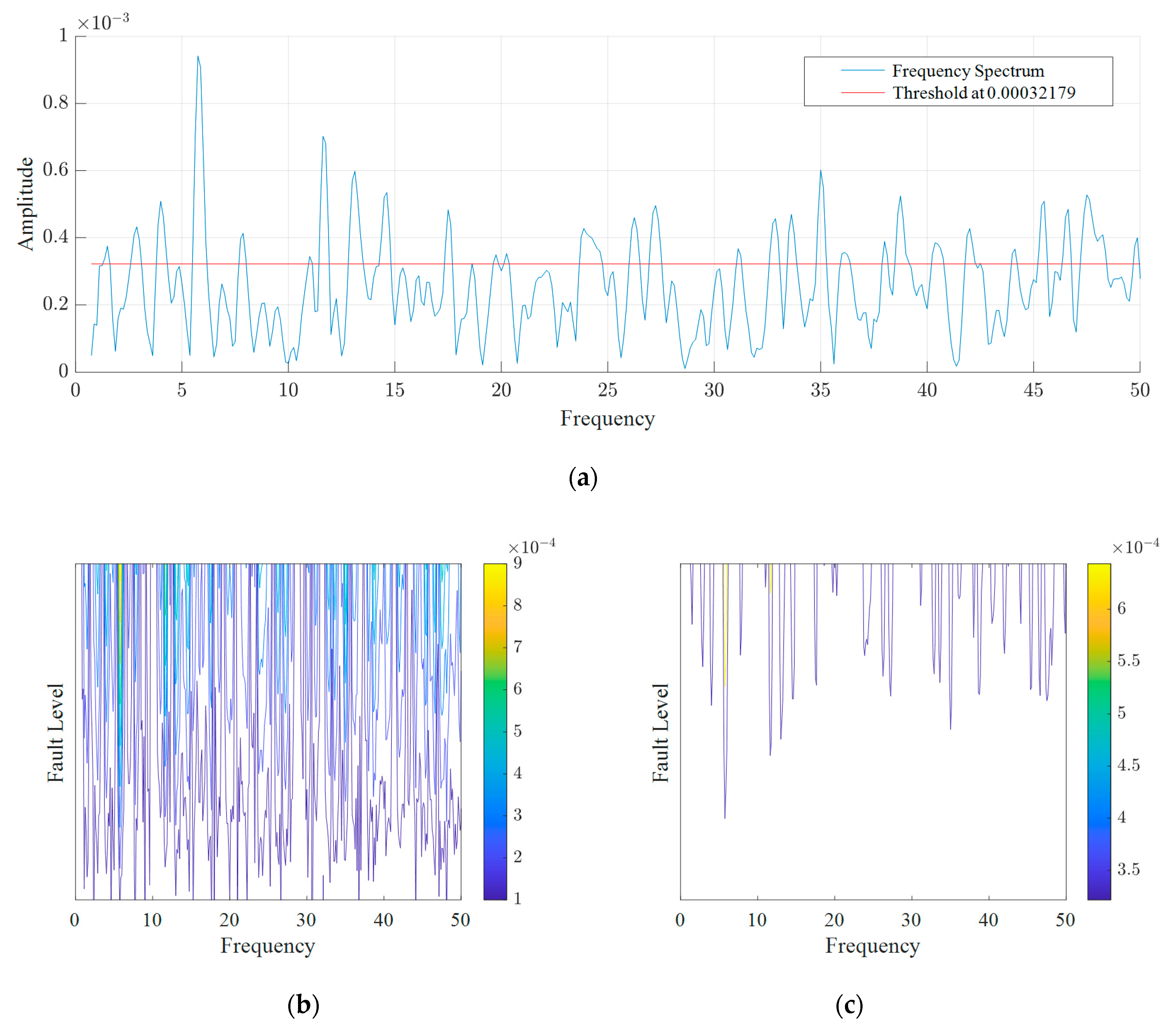
In the spectrum segment represented in Figure 7a, it can be observed that the maximum frequency amplitude slightly exceeded the value of 9 × 10⁻⁴, establishing a contour interval between isolines of 1 × 10⁻⁴; however, the use of this spacing involves a large amount of noise, such that its corresponding contour map is marked by a high density of isolines (Figure 7b), whose information is largely contaminated by noise. On the contrary, defining a threshold makes it possible to obtain a clearer contour map, such as that seen in Figure 7c.

2.5.1. Lower Boundary

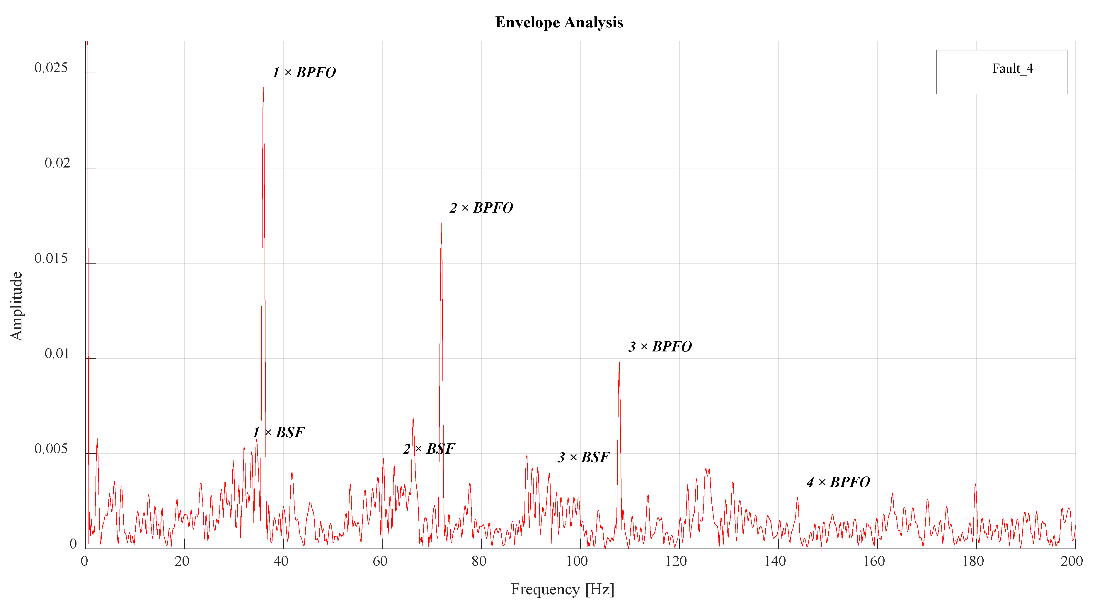
Guilbert [39] considered that the construction of a contour map should begin with the determination of the lowest isoline value, which is necessary to establish a lower bound (or threshold) that allows for the identification of representative amplitudes. As the main purpose of Envelope Analysis is to detect resonant zones modulated in amplitude by periodic impact forces, the representative information in the envelope spectrum will be observed at low frequencies. Figure 8 shows how the amplitudes of a section of the envelope spectrum have a significant amplitude (associated with a fault frequency and its harmonics); as the frequency increases, these amplitudes decrease.

This makes it necessary to determine a section of frequencies to be analysed, whose amplitudes provide information of interest. In the estimation of the lower limit of the section ($S_{low}$), the frequency response of the piezo-ceramic accelerometer used in this study, whose linearity is above 0.4 Hz, was considered. On the other hand, the upper section limit ($S_{up}$) was determined by considering the maximum operating rotation frequency ($F_r=8.33 \mathrm{Hz}$) and the bearing characteristics, such as the number of rolling elements ($N_b=15$) and Ball Pass Frequency Inner ($BPFI=8.8148·F_r$), given that it has the highest decay constant (Table 3):

$$S_{up}=N_b·BPFI.$$

(1)

Thus, the estimated section considers all the possible fault frequencies of the bearing and its harmonics, within its operating range.

This consideration allows the threshold to adapt to the change in spectrum amplitude, depending on the fault in the record to be evaluated. For this, a previous analysis was implemented, based on the distribution of amplitudes in the spectrum, using a frequency table. We make some definitions, as follows:

• The sample (X) is a data set of length N, which is used in the analysis of the distribution of the amplitudes. These data correspond to the amplitudes of the frequencies from $S_{low}$–$S_{up}$.
• The range ($R_a$) corresponds to the difference between the frequencies of maximum and minimum amplitude.
• The number of intervals ($N_{int}$) is defined by the range and the mean value of the amplitudes analysed:

  $$N_{int}=\frac{R_a}{\frac{{{\displaystyle \sum }}_{ Rai=1}^N{X}_i}{N}}.$$

  (2)
• The width between intervals ($I$) is described by the division between the range and the number of intervals:

  $$I=\frac{R_a}{N_{int}}.$$

  (3)

Once these criteria have been considered, the frequency distribution table is generated, from which the arithmetic mean ($\overline{x}$) of the amplitude distribution must be obtained, where $x_i$ is the mean between the extremes of the interval, $f_i$ the number of components that belong to each interval and $N$ the number of elements in the sample:

$$\overline{x}=\frac{{{\displaystyle \sum }}_{i=1}^N{x}_i·f_i}{N}.$$

(4)

Subsequently, in the final stage, the amplitudes that exceed the value of the arithmetic mean are identified; thus, establishing a new data set (X₂), whose mean will correspond to the threshold value:

$$Threshold=\frac{{{\displaystyle \sum }}_{i=1}^{N_2}{X}_2}{N_2}.$$

(5)

2.5.2. Upper Boundary

The upper limit represents the value to which the isolines that make up the contour map will extend. This limit can be obtained from the registry to be evaluated, thereby reducing the computational cost; however, this may lead to confusion in the interpretation of the data, since there would be no continuity in the evolution of the fault, such that the contour map would be incomplete.

In this study, it is considered that the upper limit is related to the frequency of maximum amplitude, obtained from the records that make up the contour map. This is because the amplitude generated is related to the impact force of a severe fault. In this way, continuity will be presented in the failure evolution.

2.5.3. Contour Interval

As stated previously, contour maps have a constant isoline spacing value, called the contour interval. Before estimating the contour interval, it is necessary to determine the number of isolines ($N_{iso}$) that allow a correct distribution of the data in the analysis. From experience, we recommend the use of $N_{iso}<20$, a value consistent with the Sturges rule [56]. This rule is simple and is based on the number of samples N analysed, previously determined in the elaboration of the frequency table:

$$N_{iso}=1+3.322·lo{g}_{10}\left(N\right).$$

(6)

Once N_iso is determined, this value must be converted to an integer, rounding to the nearest odd integer. Subsequently, the contour interval is determined, as indicated in Equation (7), to establish the set of values of each isoline with said value.

$$Contou{r}_{Interval}=\frac{Uppe{r}_{Boundary}-Threshold}{N_{iso}}.$$

(7)

2.5.4. Isoline Value

The value of each isoline is defined by a set of values, established using the multiples of the contour interval and the lower limit or threshold, without these exceeding the upper limit. This relationship is presented in Equation (8), where $k=0,1,2,3,\dots$, represents the multiple of the spacing value:

$$Isolin{e}_{Value}=Threshold+k·Contou{r}_{Interval}.$$

(8)

2.6. Determination of Analysis Points

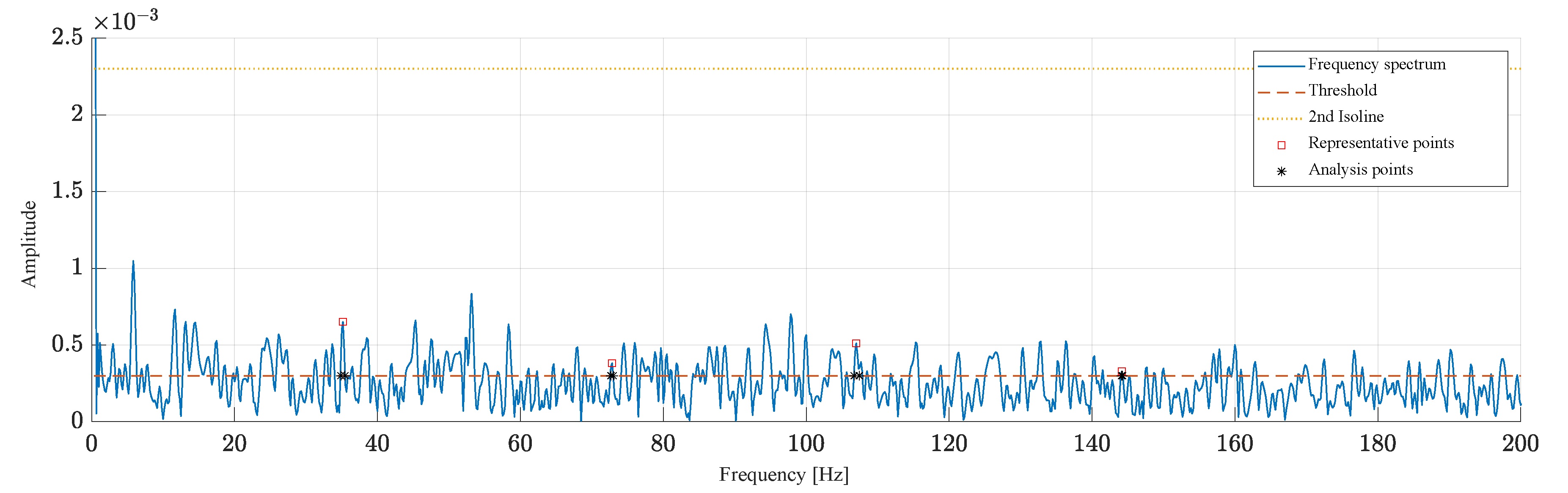
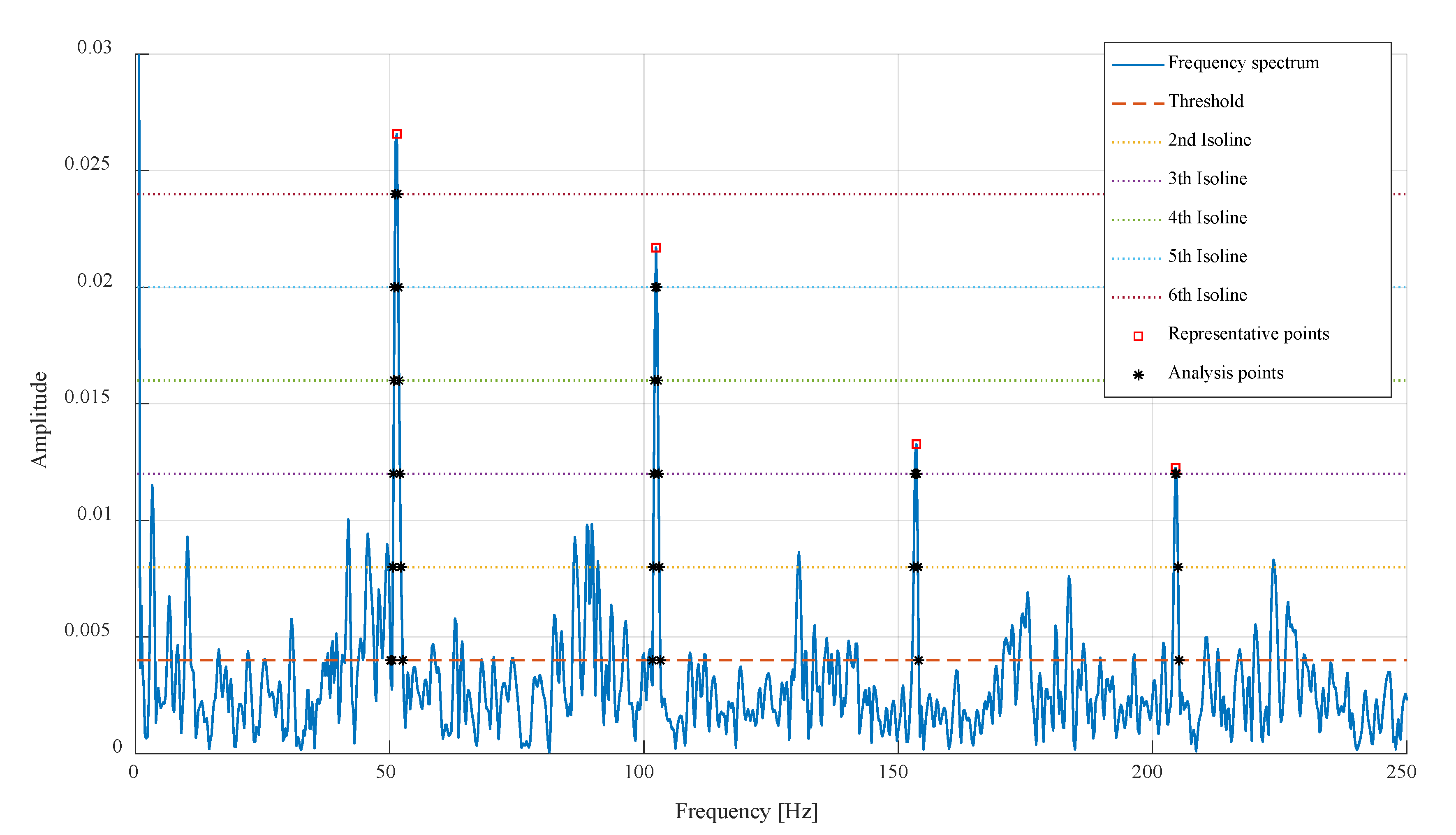
The analysis points are defined as the intersection between the set of isoline values and the amplitude of the evaluated frequency. Later, these analysis points will be used to establish the relationship between the evaluated record and the contour map. For this, it is necessary to determine the representative points, associated with the maximum amplitude of the fault frequency and its harmonics. 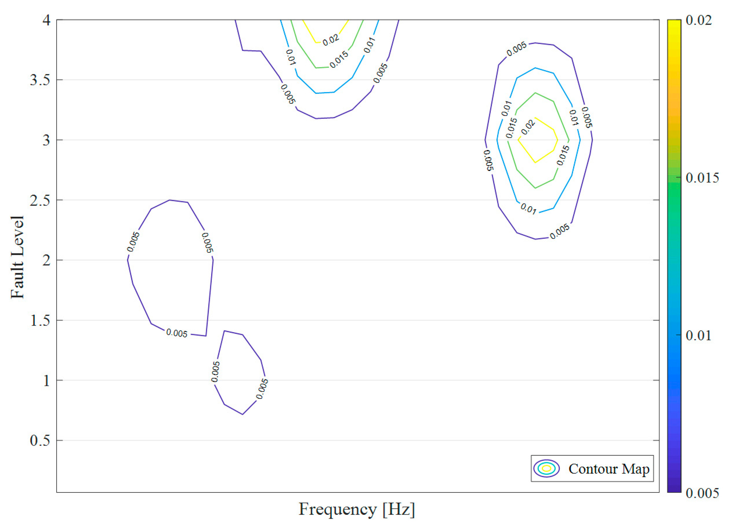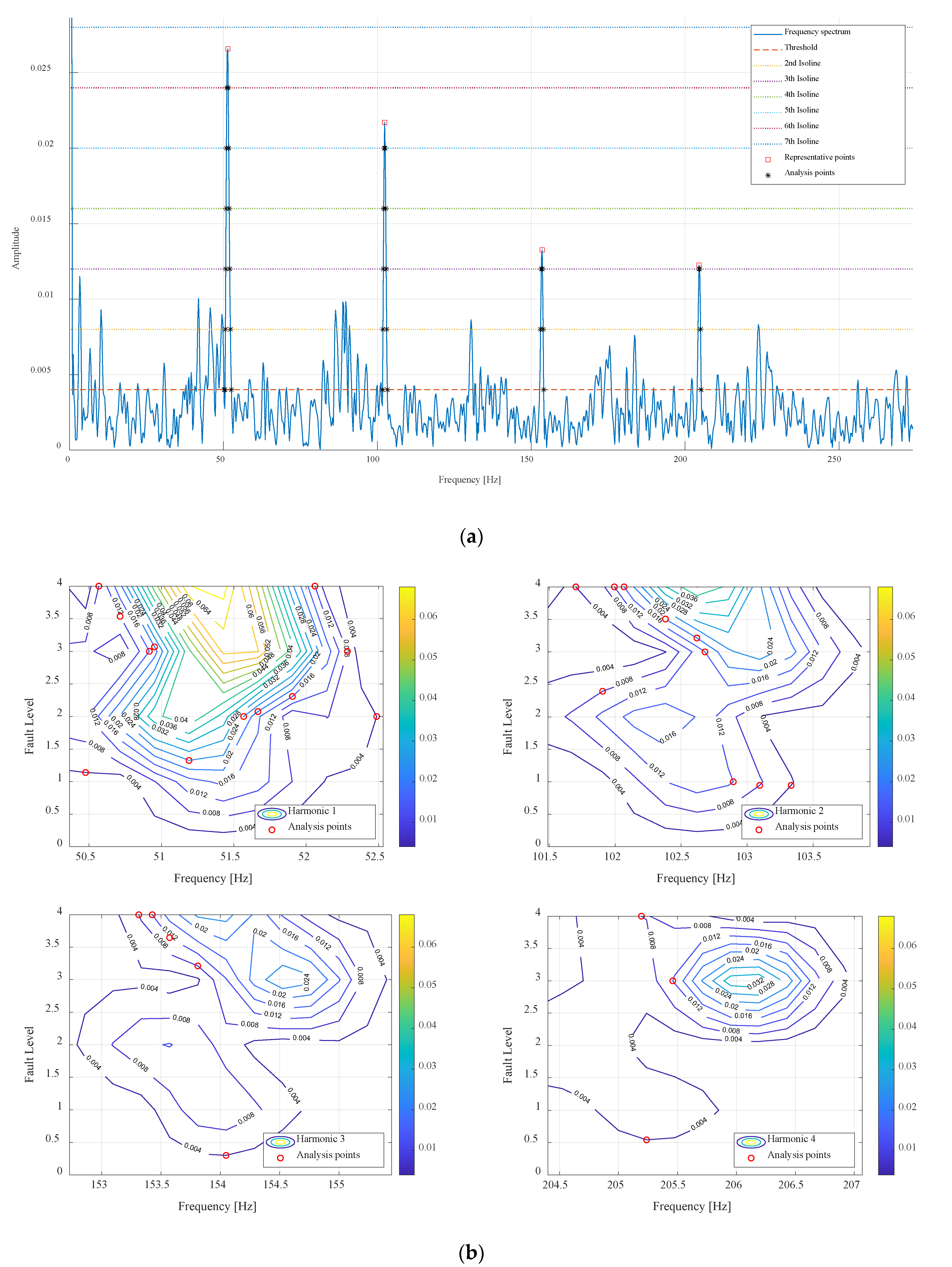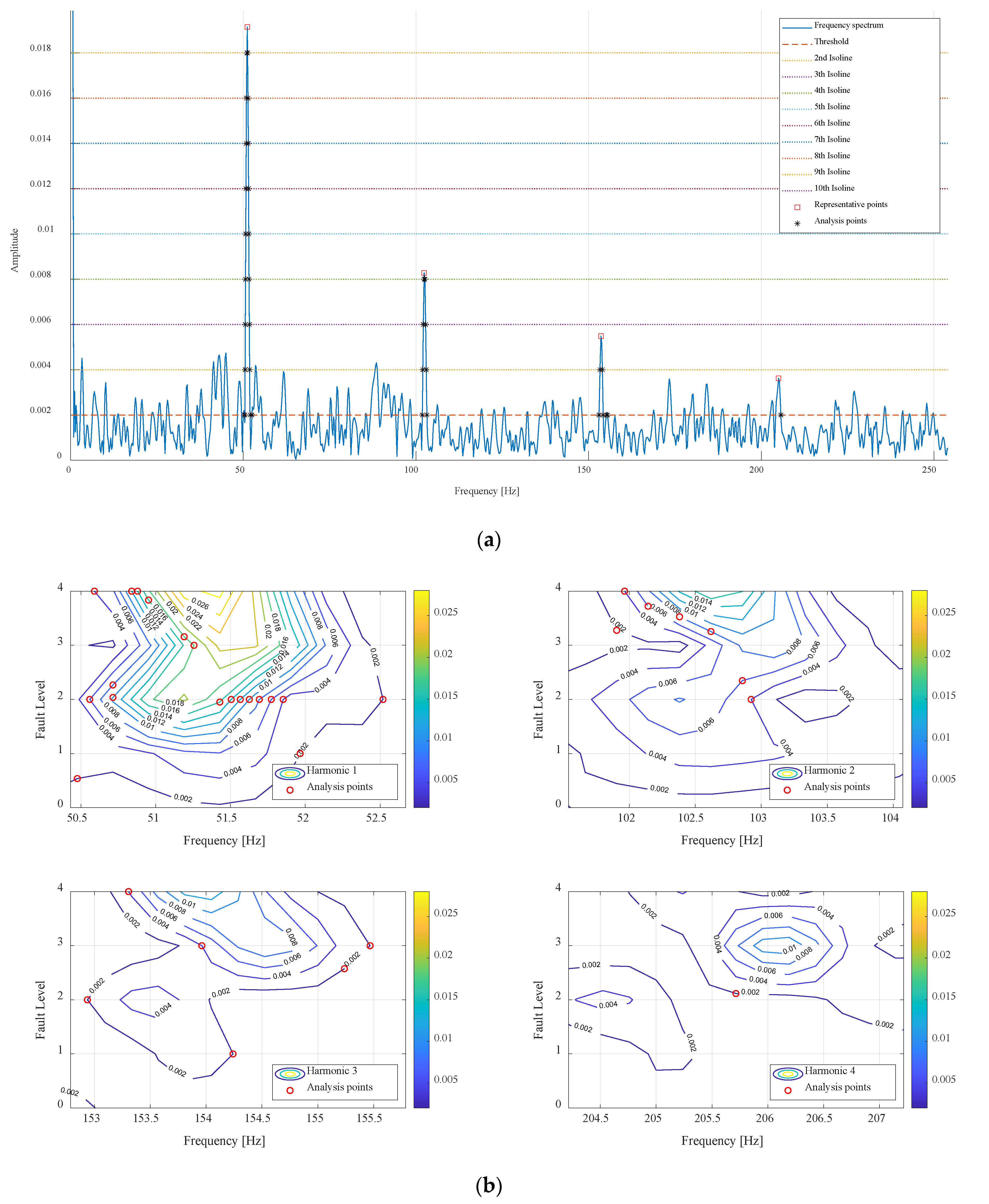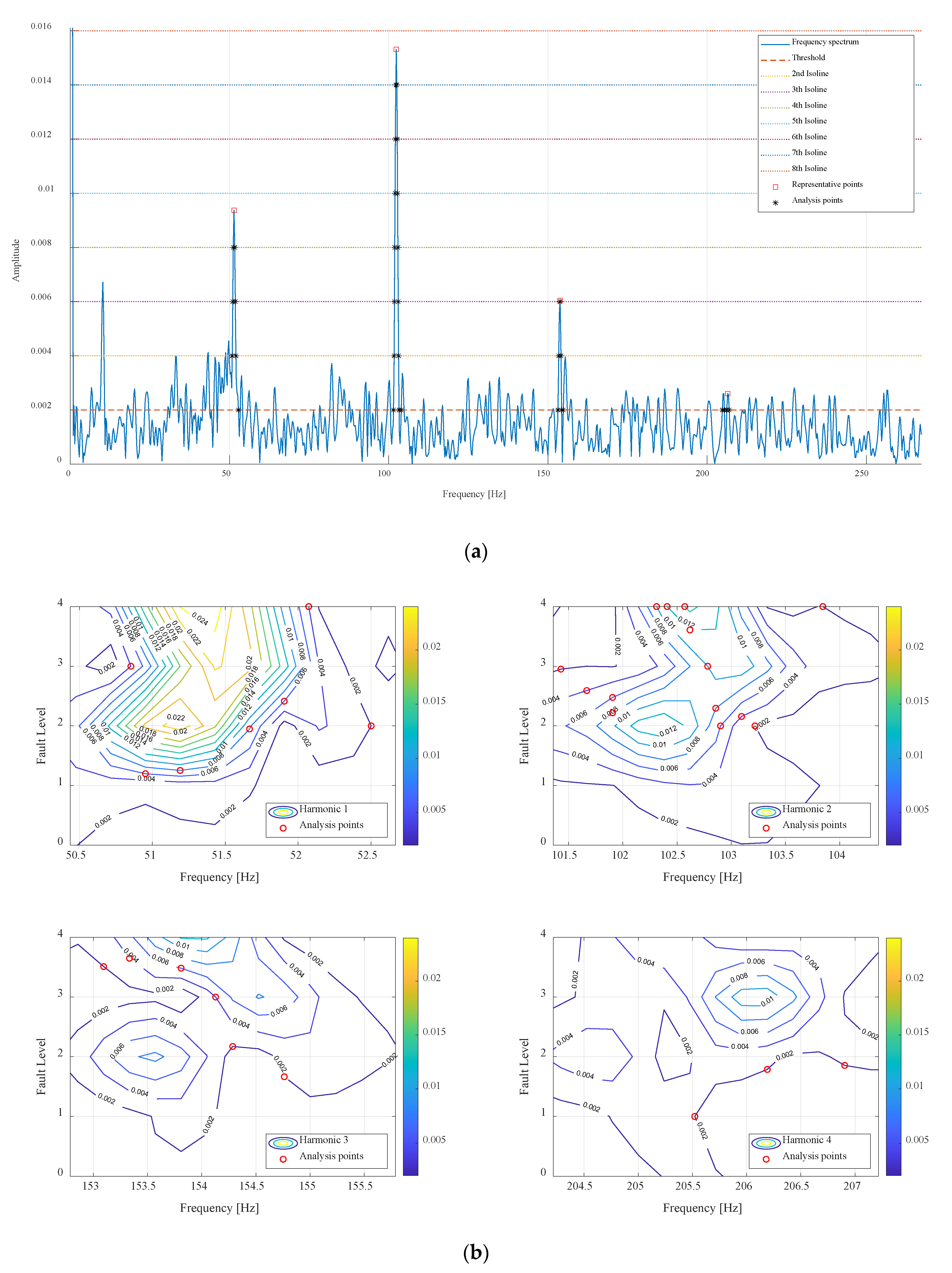Figure 9 presents a vibration record with a rotation speed of 500 rpm and failure level of 2, where the analysis points correspond to the intersection between the value of the isolines and the amplitude of the failure frequency and Harmonics.

2.7. Example of Contour Map Set-Up

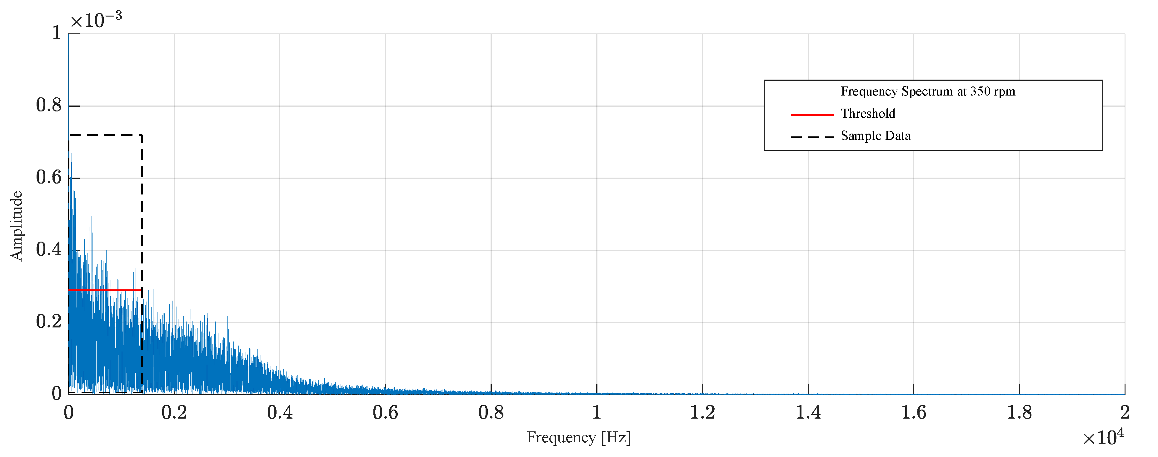
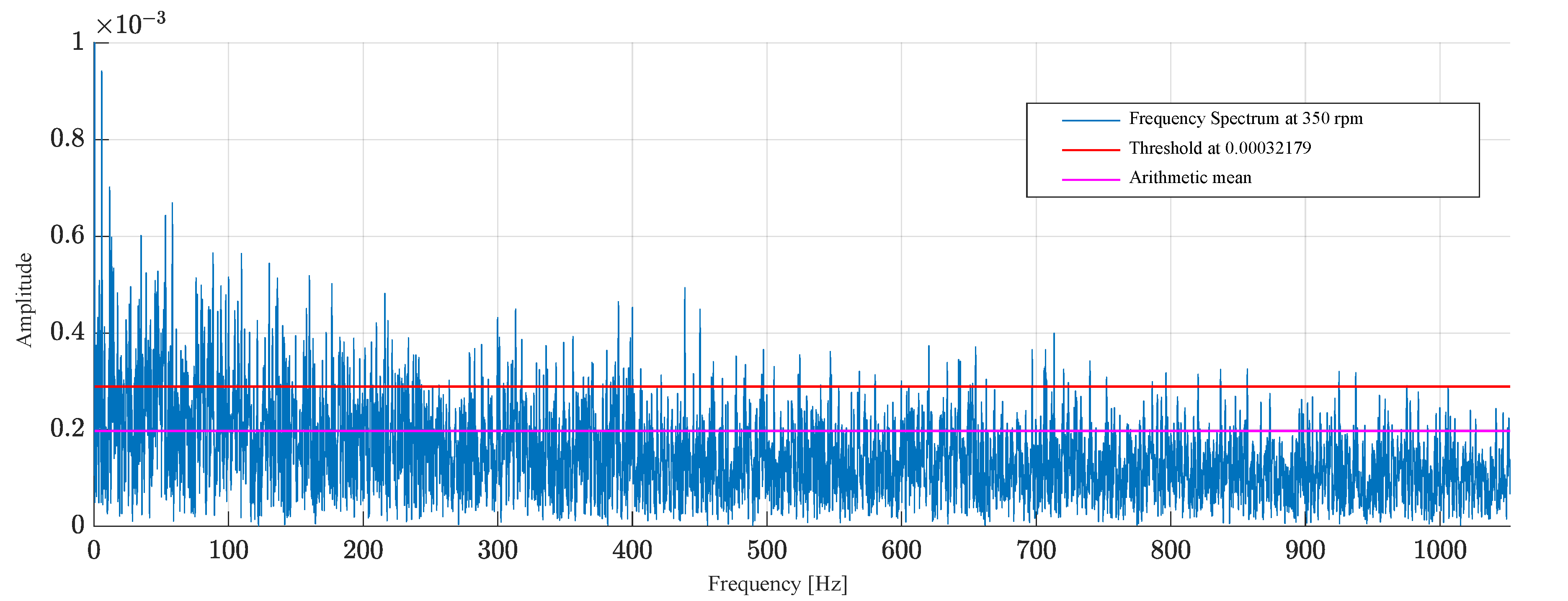
This section presents an example of the estimation of the aforementioned criteria, based on a record of the normal running state of the bearing operating at 350 rpm, as indicated in Figure 8. As a starting point for the construction of the contour diagram, the threshold value of significant amplitudes should be determined.

For this purpose, we considered the characteristics of the accelerometer, estimating the lower limit of the section under analysis ($S_{low}=0.4 \mathrm{Hz}$). Similarly, starting from Equation (1) and knowing that $BPFI=73.46 \mathrm{Hz}$ (Table 3), $S_{up}=1101.9\approx 1100 \mathrm{Hz}$ was obtained. Considering the selection criteria of the data set, it was estimated that the analysis sample is made up of the amplitudes of frequencies from 0.4–1100 Hz, as shown in Figure 10.

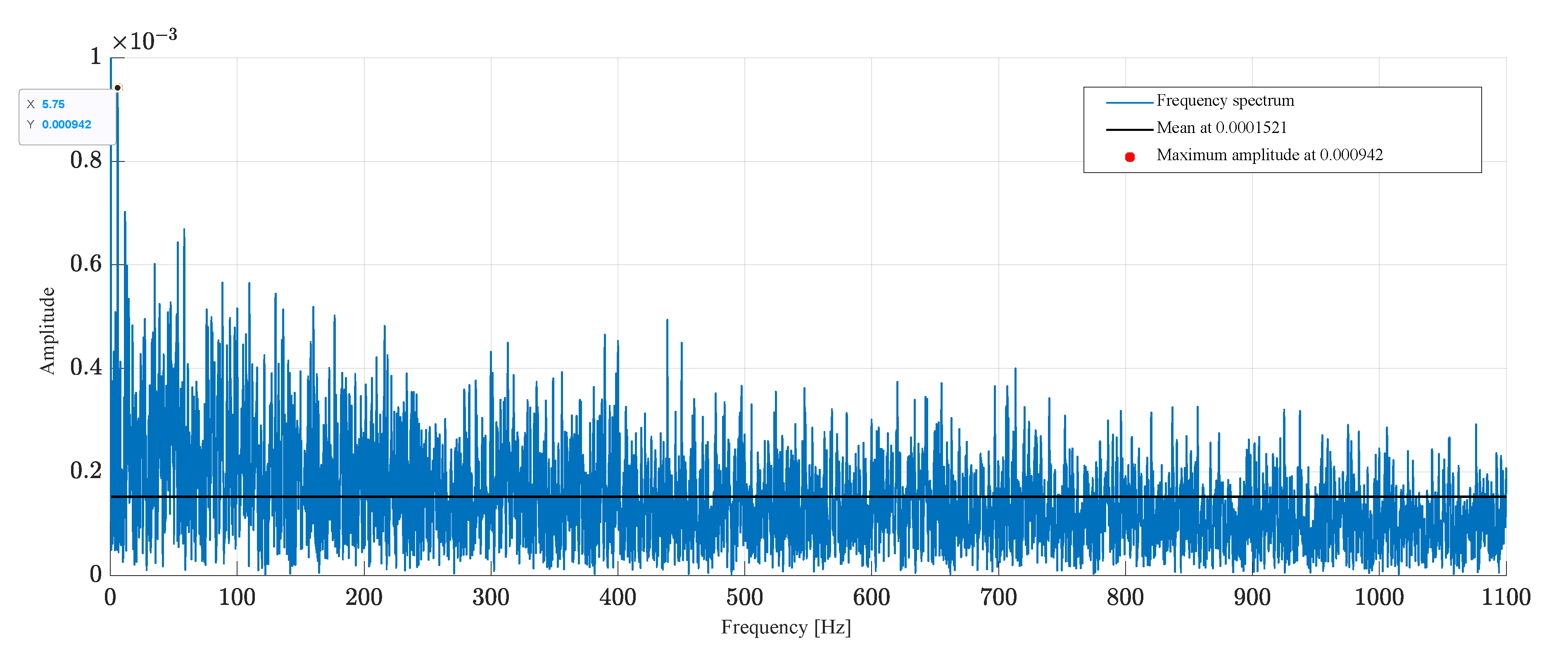
The range (R) corresponds to the maximum amplitude of the spectrum, with a value of $9.41\times {10}^{-4}$, and the mean value of the amplitudes of the sample was 1.521 × 10⁻⁴, as can be observed from Figure 10. From this, using Equation (2), the number of intervals ($N_{int}$) could be determined, which, in this case, was 6. With this and Equation (3), it was estimated that the amplitude between intervals was 0.000157. Next,

Table 7. Frequency distribution.

Interval	${\mathit{x}}_{\mathit{i}}$	${\mathit{f}}_{\mathit{i}}$	${\mathit{f}}_{\mathit{i}}·{\mathit{x}}_{\mathit{i}}$
0–0.000157	7.8499 × 10−5	1.5529 × 105	12.19
0.000157–0.000314	0.0002355	4183	0.98509
0.000314–0.00047099	0.0003925	462	0.18133
0.00047099–0.00062799	0.00054949	56	0.030772
0.00062799–0.00078499	0.00070649	6	0.004239
0.00078499–0.00094199	0.00086349	2	0.001727

shows the frequency distribution based on the aforementioned parameters, where $x_i$ represents the mean value of the interval, $f_i$ is the absolute frequency or number of elements contained in each interval and $f_i·x_i$ is the product between the mean value and the absolute frequency.

Subsequently, using Equation (4), the arithmetic means of the grouped data set was determined, the value of which was 2.13 × 10⁻⁴. This magnitude was used to identify the amplitudes that exceeded said value, establishing a new data set. Then, using Equation (5), the threshold value was estimated; which, in this case, was 3.218 × 10⁻⁴, as indicated in Figure 11.

Subsequently, the upper limit was established, identifying the maximum amplitude-frequency of the registers that make up the contour map under the operating conditions analysed. Given that, in this case, the degradation of a fault at 350 rpm was evaluated, in Figure 12 it can be observed that the maximum amplitude-frequency corresponds to a fault level of 4.

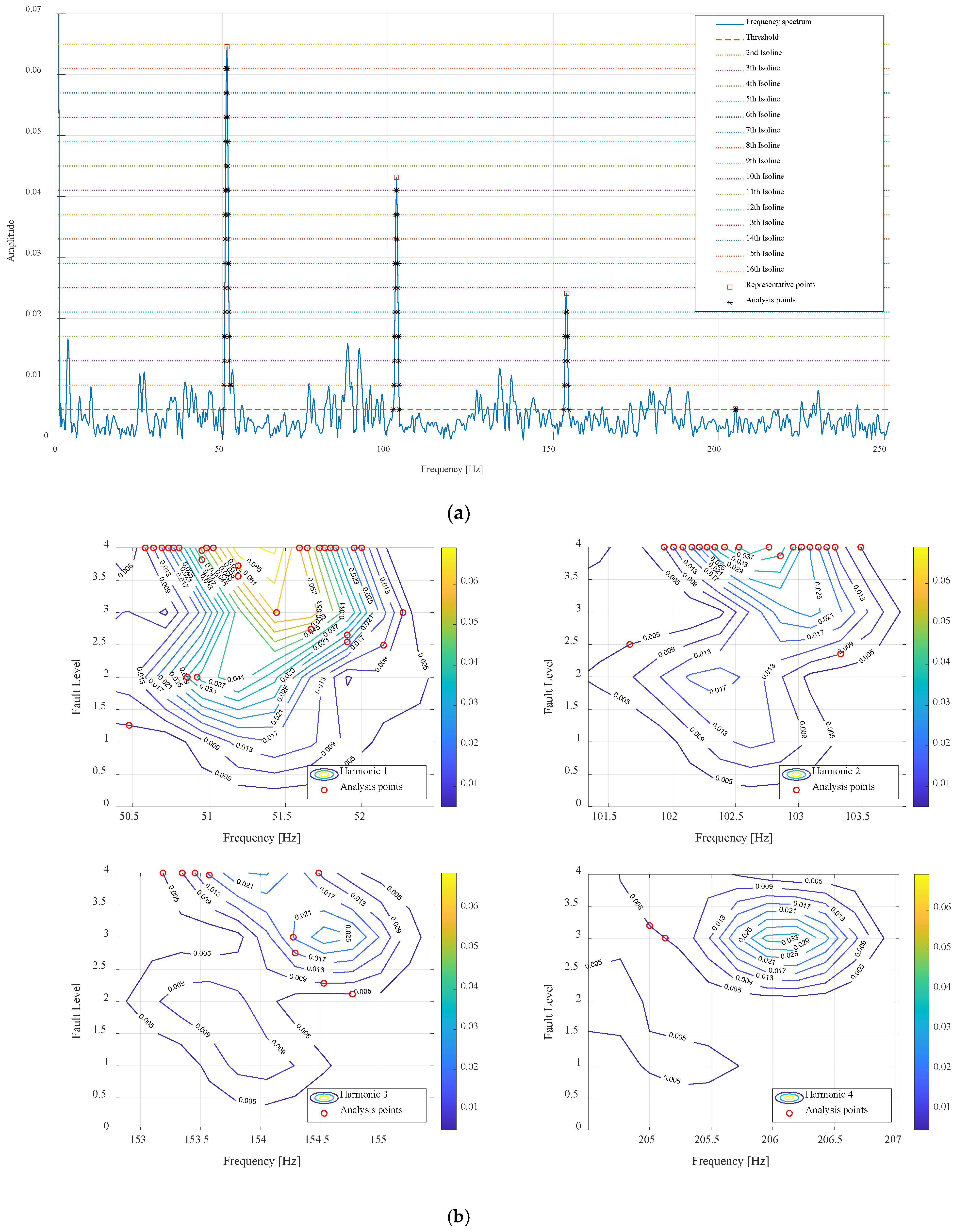
Once the threshold and upper limit were identified, we proceeded to determine the number of isolines to make up the contour map. Starting from Equation (6), and considering the length of the sample, $N_{iso}=13$ was estimated. Thus, the value of the contour interval was estimated as 0.0049. Subsequently, the set of isoline values was established, starting from the threshold value, and the intersection points of the isolines and the amplitudes of the spectrum under analysis were identified (Figure 13).

3. Results

The following section presents the results obtained in the validation of the method proposed in this study. In the first section, the characteristic failure mode of the case study is described and the component on which the analysis is focused is determined. Afterwards, the results obtained in the bearing diagnosis by means of contour maps at 500 rpm are presented, for five fault levels from F4 to F0. Subsequently, considering a difficult-to-diagnose case, the influence of the filter band (using bands proposed in [16]) on the diagnostic capability of the proposed method is analysed. Finally, considering a difficult-to-diagnose fault level, it is analysed whether the same behaviour exists at different speeds (200 and 350 rpm), maintaining a filtering band of 1.8−6.1 × 10³ Hz. For each studied case, the measurements were composed of three replicates, one of them was used in the creation of the contour map, and the remaining replicates were used to validate the proposed diagnostic method.

3.1. Failure Characterisation

The study of the influence of localised defects on the vibration signature of a bearing is a frequently addressed topic [57]. In the presence of a localised fault, the modulation phenomenon is triggered, produced by periodic impacts that excite the bearing resonance frequencies. Smith and Randall [54] have described the vibration modes of a bearing, under localised failure in each component, using envelope analysis. For defects in the outer race, the fault frequency will have side bands modulated to the frequency of rotation of the shaft in its first harmonics. In the case of failure in rolling elements, although the envelope spectrum should present harmonics with side bands modulated at the cage frequency, it presents impulsive content. Another characteristic considered in the vibration mode of rolling elements is the presence of harmonics of the cage frequency [16].

However, a problem arises when diagnosing a combined defect, due to the interference that can occur between the vibration modes of the affected components. As detailed in Section 2.2.2, in this study, we analysed a combined outer race and rolling element fault. Figure 14 shows a vibration spectrum at 350 rpm. For both failure cases, there were changes in the failure mode. The Outer Track Fault Frequency (BPFO) harmonics no longer have sidebands spaced at the shaft turning frequency. In contrast, for rolling elements, harmonics corresponding to the frequency of the cage were not observed, and only the impulsive content of the lateral bands of the rolling elements failure frequency (BSF) was evident.

On the other hand, it is important to highlight that although both components presented the same level of severity, the amplitude of BPFO was predominant, in comparison with BSF. This is why this study focused on the diagnosis of failure in the outer race, considering the diagnosis of failure in rolling elements in future works.

3.2. Diagnosis of Fault Levels for 500 rpm with Filter Band at 1.8–6.1 × 10³ Hz

3.2.1. Diagnosis for a Level 4 Fault at 500 rpm

Figure 15a presents the spectrum of the case study, where the analysis points or intersection between the different isolines and the amplitudes associated with the fault frequency and harmonics are represented, which are evaluated in the contour map. Figure 15b shows that the corresponding fault level is determined for each harmonic from the value of the isolines and the frequency of the analysis points. Although it is true that there were coincidences of the analysis points with failure levels that did not correspond, these coincidences were associated with low-value isolines. On the other hand, the highest concentration of analysis points corresponded to the fault analysed, being associated with isolines with significant values.

3.2.2. Diagnosis for a Level 3 Fault at 500 rpm

Figure 16 presents the spectrum diagnosis of the case under analysis in its respective contour map. This shows a clear concentration of the analysis points on the fault level evaluated in each of its harmonics. As in the previous case, there were outliers; however, their isoline values were low.

3.2.3. Diagnosis for a Level 2 Fault at 500 rpm

For this case of analysis, Figure 17a represents the spectrum of the case under study, where the presence of the fault frequencies associated to the two evaluated components (BPFO and BSF) was observed. Figure 17b shows that the notable presence of the BSF component significantly influenced the diagnosis. Although analysis points with high isoline values coincided with the evaluated case in failure frequency, the dispersion of the remaining analysis points made the diagnosis difficult. Therefore, in Section 3.3, the influence of the filtering band on the diagnosis is further analysed.

3.2.4. Diagnosis for a Level 1 Fault at 500 rpm

This case was similar to the level 2 fault spectrum. However, in Figure 18, in the fundamental frequency of failure, a greater concentration of points was observed at the level of the case analysed (Level 1); however, for the other harmonics, the spread of points may confuse.

3.2.5. Non-Fault Register Diagnostics at 500 rpm

Figure 19 shows the diagnosis of this analysis case, where it was observed that the representative points associated with the fault frequency and the fourth harmonic slightly exceeded the threshold value. Consequently, the evaluation of the correspondence of the analysis points showed a null significance on the contour map.

3.3. Diagnosis of Failure Levels for 500 rpm at Different Filter Bands

As previously stated, given the inconvenience in the diagnosis of level 1 and 2 failures, a study was carried out to analyse the influence of the filtering band on the diagnosis using contour maps. Three filtering bands are studied in the following sections.

3.3.1. Diagnosis for a Level 2 Fault in the Frequency Band of 0.2–1.8 × 10³ Hz

As Figure 20 shows, lowering the filter band is not an option when diagnosing a fault using contour maps. This is due to the presence of a large amount of noise, which distorts the analysis frequencies.

3.3.2. Diagnosis for a Level 2 Fault in the Frequency Band of 6.1–9.2 × 10³ Hz

Figure 21a shows an obvious improvement in noise, where the amplitude of the fault-associated frequency (BPFO) is clearly significant, while the BSF frequency is overshadowed by the noise. This results in a higher concentration of the analysis data in the case study in the contour diagram, as can be seen in Figure 21b.

3.3.3. Diagnosis for a Level 2 Fault in the Frequency Band of 9.2–12.8 × 10³ Hz

In this case, the noise increased as the filter frequency band increased, as shown in Figure 22a. This caused problems in the diagnosis of the registry, which can be seen from Figure 22b. However, this increase in noise was associated with the characteristics of the accelerometer used, as it has a response frequency of up to 10 kHz.

3.4. Diagnosis for a Level 2 Fault at 200 and 350 rpm (Frequency Band of 1.8–6.1 × 10³ Hz)

This section analyses the influence of the rotation speed in the fault diagnosis, specifically for fault level 2, given the inconveniences observed in the analysis at 500 rpm. In both cases, the concentration of the analysis points was associated with the level of failure under study. However, at 200 rpm, there was a higher concentration of points in the fundamental fault frequency; see Figure 23a. On the other hand, the record at 350 rpm—as shown in Figure 23b—presented a behaviour similar to that at 500 rpm, where there was dispersion in the analysis points; however, for this case, although dispersed, they were closer to the studied failure level.

4. Discussion and Conclusions

In this work, a methodology was developed to represent the levels of failure of a bearing by means of contour maps which relate the level of failure, the frequency and its amplitude as a function of isolines. This methodology was applied to a real case of experimental acceleration measurements from a bearing test bench. Furthermore, within these contour maps, the points of registers other than those used for their generation were represented, observing coherence in all analysed cases. Therefore, the results suggested that this methodology can help in the prediction of bearing failures.

The data presented were analysed by envelope analysis in different filter bands, which showed the influence on the identification by the specific bands, in cases of diagnostic confusion, such as that which occurred for failure level 2 at 350 rpm and 500 rpm. Another important feature to highlight is the increased diagnostic accuracy for high-level (3 and 4) failure cases evaluated at 500 rpm.

Table 8. Setting the conditions for the analysis of the case studies.

Regime [rpm]	Fault Level	Filter Band [Hz]	Window Width [s]	Threshold
500	F4	1.8–6.1 × 103	2.1	0.005
	F3	1.8–6.1 × 103		0.006
	F2	1.8–6.1 × 103		0.004
	F1	1.8–6.1 × 103		0.004
	F0	1.8–6.1 × 103		0.0005
	F2	0.2–1.8 × 103	2.1	0.009
		6.1–9.2 × 103		0.002
		9.2–12.8 × 103		0.002
350	F2	1.8–6.1 × 103	3	0.002
200		1.8–6.1 × 103	5.25	0.0004

summarises the study conditions of the analysed cases described in Section 3, where it is observed that the threshold value is closely related to the rotational speed, fault level, filter band and the window width employed in each analysis. The filter bands used in this analysis are those proposed in a previous study [16]. The width of the analysis window corresponds to the time spent at each determined rotation speed for turning a total of 17.5 turns. The threshold value is determined with the criteria described in Section 2.5.1 and depends on the vibration index at each fault level.

A clear advantage of the implementation of contour maps in fault diagnosis is the significant data reduction, which depends on the correct identification of the threshold, by suppressing the data associated with noise. Furthermore, when analysing the harmonics associated with the failure frequency, the importance of the behaviour of the isolines was demonstrated: for the same frequency, there are amplitudes associated with different levels of failure—that is, the relationship between frequency and amplitude with the level of failure is not biunivocal—which explains the difficulty of identifying the level of failure according to which frequency is being analysed. This methodology makes it possible to identify isoline behaviour patterns, establishing frequency sections associated with harmonics, to unambiguously study the evolution of a bearing failure.

The proposed method allows classifying the level of bearing failure using many points (intersection between the value of the isolines and the amplitude of the frequency and its harmonics). Based on the preliminary results, the proposed direct calculation method has been quite accurate in its diagnosis. Although this method requires an operational history, it has several advantages compared to indirect diagnostic methods based on artificial intelligence. On the one hand, the analysis is deterministic, allowing an easy interpretation of the results by the analyst and thus, ruling out uncertainty in decision-making, such as what happens in the black box in neural networks. Also, since no prior training is required, it is not necessary to label a large amount of data. The presented treatment is generic and could be used in the monitoring of a wide range of mechanical equipment, where the status of its components could be classified by changes in the amplitude of their working frequency. However, in the future, the information of the presented treatment could also serve as input/output of an artificial intelligence system.

Although the initial results of a methodology that is in active development were presented, the results observed so far meet our expectations and lead us to think that implementing other criteria, such as the slope between isolines, the distance between analysis data and correct identification of filter band (spectral kurtosis), can improve the diagnostic accuracy. Analysis of the influence of the load and lubricant film on the behaviour of the contour maps is also a topic of interest and we are planning new tests in this regard. The behaviour of the contour maps for variable speed cases will be further studied in future research. Other considerations for the proposed method are related to establishing more robust criteria to determine the analysis section, identification of sections with constant velocity, and the control of uncertainty in the identification of failure frequencies. These criteria will be also considered in future works.