Numerical Analysis of the Take-Off Performance of a Seaplane in Calm Water

Featured Application

This paper provided a numerical approach to predict the resistance and attitude of a seaplane taking off in calm water. The investigations on take-off performance of the seaplane would provide some guidance in the integrated design of aerodynamics and hydrodynamics of the seaplanes.

Abstract

Nowadays, with the escalating tensions in maritime dispute and the development of marine economy, there has been renewed interest in seaplanes for their special capacity of taking off and landing on water. Prediction of take-off performance, involving aerodynamic analysis and hydrodynamic analysis, is a main challenge in seaplane design, while the prediction methods have been little improved since the 1960s. This paper aims to investigate the attitude and resistance characteristics of a seaplane at different speeds during the take-off by numerically modeling the air-water flow field using RANS equations with VOF method. The trim and heave motion of seaplane in response to aerodynamic forces, hydrodynamic forces, hydrostatic forces, and propeller thrust was realized by solving rigid body dynamics equations and adopting dynamic overset mesh technique. The variations in heave, trim angle, and resistance characteristics during the takeoff were investigated, and their inherent relationships with the aerodynamic, hydrodynamic, and hydrostatic performance were revealed. Particular investigation on the hydrodynamic resistance indicates that the stagnation line located at the convex bow would contribute a considerable increase of pressure resistance at the first hump, and the trim angel of a seaplane should be operated in an optimum trim range, typical between 4–6 deg, to minimize the hydrodynamic resistance at the second hump. Additionally, the dynamic motion convergence study proves that the utilization of damping terms was an effective way to accelerate the convergence of the dynamic motion ending with a quasi-static state.

1. Introduction

Seaplanes are powered fixed-wing aircraft capable of taking off and landing on water. They once played an important role in the early stage of modern aviation. But the rapid development of land-based aircraft and the growing investments in airports after WWII drastically reduced the demand for seaplanes, which resulted in the stagnation of seaplane technique for nearly half a century [1]. Recently, the development of the marine economy and the escalating tensions in maritime disputes has drawn people’s attention back to water-based aircrafts for their wide applications in military and civil fields, such as maritime reconnaissance, anti-submarine, logistics service, sea rescue, etc. [2].

The design of a seaplane is an art of tradeoff between aerodynamics and hydrodynamics with the ultimate goal to achieve the desired hydrodynamic performance with the least loss in aerodynamic efficiency. The main challenge faced by designers for evaluating the take-off performance is the prediction on the resistance characteristics, since during take-off the seaplane is free to trim and heave in subject to the forces of hydrodynamics, hydrostatics, aerodynamics, and propulsion system. Evaluation of hydrodynamic performance is the most challenging job because the seaplane disturbs the water surface into complicated wave flow that is difficult to predict. It is known that besides the fuselage geometry, the hydrodynamic resistance mainly depends on speed, water load, and trim angle which is defined as the angle between the keel of forebody and the water level. The water load and trim angle would be influenced by the aerodynamic lift and pitching moment respectively, which basically results in the coupling of hydrodynamic performance and aerodynamic performance that makes the prediction more complicated [3].

There are three available methods for investigating the resistance characteristics of seaplanes: experimental method, empirical method and numerical method.

Towing tank tests are the common experimental implements to investigate the resistance characteristics of seaplanes in take-off. Since the towing tanks always have a limitation on the model scale and planing speed, a dilemma that researchers have to face in the scaling model tests is the inability to satisfy the similarity of theFroude number and Reynold number [4]. Moreover, the experimental method is too expensive and time-consuming for the preliminary design and optimization of a seaplane.

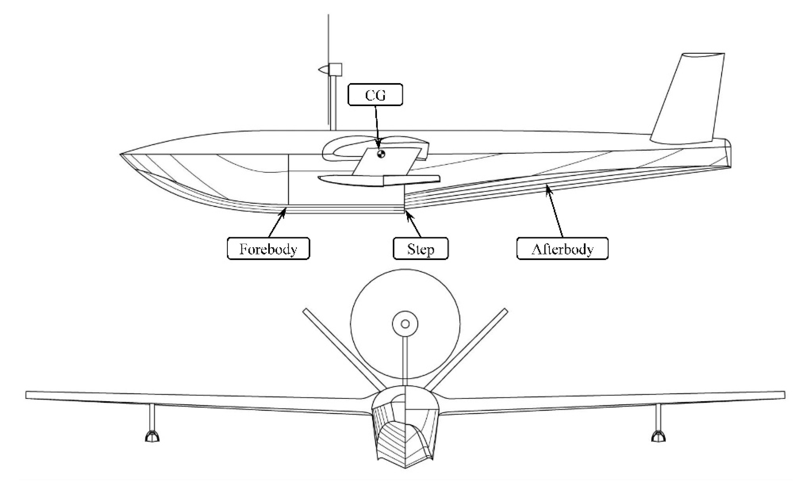
Empirical methods are more efficient for the preliminary design. Several attempts [5,6] have been made to estimate the resistance characteristics of seaplanes by adding aerodynamic models into Savitsky equations. Whereas, since the Savitsky methods were developed for the sample non-stepped planing hulls [7], the empirical methods lack accuracy for evaluating the hydrodynamics of unconventional hulls, especially for seaplane hulls characterized by a distinctive step at the bottom. The step introduces a sharp corner on the bottom which divides the fuselage into forebody and afterbody. The water flow is forced to separate at the step giving room to an air-filled cavity, which could reduce the wetted surface on the afterbody and prevent unfavorable suction that keeps the afterbody from leaving the water [8]. A recent study by Savitsky expanded the empirical methods to estimate the hydrodynamics of stepped hulls through predicting the wake profile of forebody [9]. But the application of the methods is still limited to the range of parameters which are not applicable for seaplanes.

Nowadays, numerical methods, especially Computational Fluid Dynamics (CFD) simulations, have become fundamental support for the analysis of aerodynamics and hydrodynamics. Reynolds-averaged Navier-Stokes (RANS) equations with turbulence models have been widely applied for the simulations of turbulence flow. Besides, the Volume of Fluid (VOF) method, which was proposed by Hirt and Nichols [10] in 1981, has been broadly used in solving the free surface problem.

Recently, there have been some CFD studies focused on the hydrodynamic performance of seaplane hulls. Xiao et al. [11] investigated the hydrodynamic performance of a single seaplane hull numerically and experimentally. They adopted the model with fixed trim and heave to examine the effects of velocity, trim, and draft on hydrodynamic performance. Khoo and Koe [12] investigated the hydrodynamics of a Wing-In-Gound (WIG) vehicle with towing tank experiment and CFD simulation. The fuselage together with floats were modeled resulting in the average error in trim angle and water resistance in comparison to experimental data, 4.3% and 8.4% respectively. Zheng et al. [13] verified the feasibility of URANS equations with VOF method on hydrodynamic analysis of a seaplane hull. They reported that the average error in trim angle and water resistance in comparison to experimental data are 3.26% and 3.12% respectively.

However, the numerical investigations on the take-off performance of seaplanes combining the analysis of aerodynamics and hydrodynamics have been rarely published. Qiu and Song [14] simulated the take-off process of a fixed-trim amphibious aircraft with an efficient decoupling method that calculated aerodynamic and hydrodynamic performance separately in CFX and FLUENT. Ma et al. [15] supplemented the decoupling method with an approximate equilibrium hypothesis which could efficiently estimate the acceleration in heave. It is evident that the decoupling method could save computing resources by simplifying the two-phase flow field around the seaplane, but a certain model error is expected owing to the interactions between the aerodynamics and hydrodynamics are ignored. Moreover, both studies adopted a fixed trim angle for the seaplane model, which is impractical for real operations. As the largest deviation in the resistance evaluations are related to the errors in the evaluation of trim angle, the rigid body dynamics should be introduced to determine the equilibrium trim angle of the seaplane at different speeds in response to aerodynamic forces, hydrodynamic forces, hydrostatic forces, and propeller thrust.

This paper aims to investigate the take-off performance of a seaplane in calm water by numerically modeling the air-water two-phase flow around a seaplane that is free to trim and heave at different speeds ranging from standstill to leave the water based on commercial software STAR-CCM+ 12.02. The remainder of this paper is organized as follows: First, the numerical model is introduced, and the numerical setups are reported in detail. The computational domain size, boundary conditions, and grid refinements are described. Second, the numerical model is validated with benchmark data of F6 wing body and Fridsma hull respectively. Then, the seaplane planing on speeds ranging from the standstill to the takeoff are simulated to investigate the variations in heave, trim angle, and resistance characteristics against speed. In particular, a detailed analysis of the hydrodynamic resistance characteristics is presented. Additionally, a convergence study is performed to examine the influence of initial attitude and damping factors on the convergence time of 2DOF motion.

2. Seaplane Model

The unmanned seaplane model investigated in this study is shown in Figure 1. The seaplane is a typical flying boat configuration with high-wing and V-tails. The fuselage is similar to a stepped hull where the bottom of the fuselage is divided into forebody and afterbody in order to reduce resistance at high speeds. Motor-driven propeller is high mounted above the fuselage to prevent the blades from the impact of water spray. The thrust line of the propeller is parallel to the keel. The floats on wingtip are used to keep the lateral attitude at low planing speed. Detail parameters of the seaplane model are given in

Table 1. Details of the seaplane model.

Parameter	Unit	Value
Wingspan	m	3.6
Wing area	m2	1.296
Length of fuselage	m	2.9
Beam width	m	0.26
Longitudinal position of step(measured from the nose)	m	1.35
Step height	m	0.02
Deadrise angle of forebody	deg	20
Deadrise angle of afterbody	deg	22
Afterbody keel angle	deg	8
Weight	kg	20
Pitching moment of inertia	kg·m2	7.26
Longitudinal CG(measured from the nose)	m	1.24
Vertical CG(measured from the forebody keel)	m	0.28
Distance from thrust line to CG	m	0.4
Thrust-weight ratio at rest		0.5

.

3. Numerical Model

3.1. Governing Equations

The incompressible viscous two-phase flow field surrounding the seaplane was described using the Reynold-Averaged Navier-Stokes (RANS) equations with turbulence model. The Reynolds averaged forms of mass conservation equation and the momentum conservation equation can be written as follows:

$$\frac{\partial \rho }{\partial t}+\frac{\partial {\overline{u}}_i}{\partial x_i}=0$$

(1)

$$\frac{\partial }{\partial t}\left(\rho \overline{u_i}\right)+\frac{\partial }{\partial x_j}\left(\rho \overline{u_i{u}_j}\right)=-\frac{\partial \overline{p}}{\partial x_j}+\frac{\partial }{\partial x_j}\left(\mu \left(\frac{\partial \overline{u_i}}{\partial x_j}+\frac{\partial \overline{u_j}}{\partial x_i}\right)-\rho \overline{u{\prime }_{i}u{\prime }_j}\right)+g_i$$

(2)

where, x_i and x_j are Cartesian coordinates, $\overline{u_i}$ and $\overline{u_j}$ represent the averaged components of velocity vector in Cartesian coordinates. $\overline{p}$ is the averaged pressure, ρ is the density, and g_i the component of gravity acceleration along the coordinate axes of inertia. In addition, μ is the effective viscosity coefficient of dynamic viscosity, and $\rho \overline{u{\prime }_{i}u{\prime }_j}$ represents the Reynolds stresses.

The k-ω shear stress transport (SST) turbulence model was introduced to close the equations. Concretely, the transport equations for k and ω are written as:

$$\frac{\partial }{\partial t}\left(\rho k\right)+\frac{\partial }{\partial x_i}\left(\rho k{u}_i\right)=\frac{\partial }{\partial x_i}\left({\mathsf{\Gamma }}_k\frac{\partial k}{\partial x_i}\right)+G_k-{\Upsilon }_k$$

(3)

$$\frac{\partial }{\partial t}\left(\rho \omega \right)+\frac{\partial }{\partial x_i}\left(\rho \omega u_i\right)=\frac{\partial }{\partial x_i}\left({\mathsf{\Gamma }}_{\omega }\frac{\partial \omega }{\partial x_i}\right)+G_{\omega }-{\Upsilon }_{\omega }$$

(4)

where G_k and G_ω represent the turbulence kinetic energy generation items, and ϒ_k and ϒ_ω represent the turbulence dissipation rate of k and ω, respectively.

A segregated flow solver with Semi Implicit Method for Pressure Linked Equations (SIMPLE) was used to conjugate pressure field and velocity field, and an Algebraic Multi-Grid solver was applied to accelerate the convergence of the solution. The convection terms were discretized by 2nd order upwind schemes.

The VOF method was used to capture the water-air interface by introducing a volume fraction α for each cell, defined as the ratio between the volume occupied by the phase and the volume of the control volume. When a cell is full of water, α = 1; while when the cell is full of air, α = 0; and when there is a fluid interface in the cell, 0 < α < 1. The transport equation for α is as follows:

$$\frac{\partial \alpha }{\partial t}+\nabla \cdot (\alpha u)=0$$

(5)

In each control volume, the two phases share the same velocity, pressure and temperature. Hence, the continuity and momentum equations were solved for a mixed fluid whose density ρ and viscosity μ were calculated by following equations:

$$\rho =\alpha {\rho }_w+(1-\alpha ){\rho }_a$$

(6)

$$\mu =\alpha {\mu }_w+(1-\alpha ){\mu }_a$$

(7)

The VOF model is very sensitive to the discretization of this convection term. Low order schemes often lead to smearing of the interface due to numerical diffusion, while the use of high order schemes results in numerical oscillations due to their unstable behavior. In this paper, the High-Resolution Interface Capturing (HRIC) scheme is used to discretize the convection term of volume fraction function. The HRIC scheme is currently the most successful advection scheme and is extensively used in many CFD codes. For improving the stability and robustness of the scheme, the software blends the HRIC with the upwind differencing (UD) scheme depending on the Courant-Friedrichs-Lewy (CFL) number. And an upper limit CFL_U and a lower limit CFL_L are introduced to adjust the blend. For simulations ending with a steady state, the value of CFL_U and CFL_L must be larger than the local CFL to ensure the HRIC scheme is applied. In this way, a large time step size could be used whilst a sharp interface is retained.

3.2. Rigid Body Dynamics

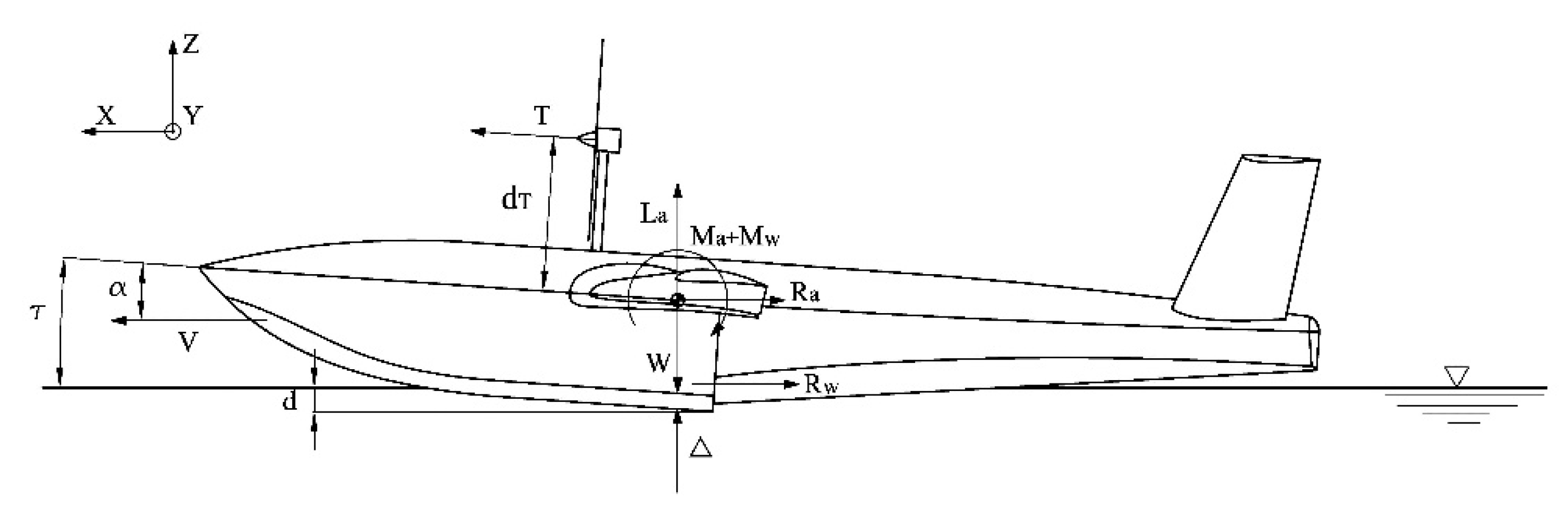
The forces and moments acting on a seaplane in take-off are shown in Figure 2. L_a, R_a, M_a are respectively the aerodynamic lift, aerodynamic resistance, and aerodynamic pitching moment acting on CG; △, R_w, M_w are the water load, water resistance, and pitching moment acting on CG produced by water, respectively; W is the weight of the seaplane, T is the propeller thrust, τ is the trim angle, d is the draft of keel at transom, and d_T is the distance between thrust line and CG.

A global fixed right-hand Cartesian coordinate system (GS) was used to describe the flow field, defined with the XZ-plane coinciding with the symmetry plane of the seaplane, and the XY-plane paralleled to the calm water surface. The positive x-axis is consistent with the velocity direction and positive z-axis points in the opposite direction of gravity. Besides, a body-fixed right-hand Cartesian coordinate system (BS) locating its origin at the CG was utilized to define the position and attitude of seaplane. The XZ-plane coincides with the symmetry plane of the seaplane. The x-axis is pointing forward in the longitudinal axis of seaplane which is parallel to the keel and the positive y-axis points to the port side. The trim angle τ is defined as the angle between the x-axis of GS and the x-axis of BS.

In order to determine the equilibrium trim angle and heave of the seaplane at different speeds, the Dynamic Fluid Body Interaction (DFBI) model was activated to simulate the 2 degree of freedom (2DOF) motion of the seaplane in response to the forces the fluid exerts and the external forces. Particularly, as we only concerned the forces at final equilibrium state, damping terms were introduced to reduce the convergence time. The governing equations for the 2DOF motion are written as follows:

$$m·\frac{\partial w}{\partial t}=F_{fluid,z}+{{\displaystyle \sum }}^{ }{F}_{ext,z}-{\xi }_w·w$$

(8)

$$I_y·\frac{\partial {\omega }_y}{\partial t}=M_{fluid,y}+{{\displaystyle \sum }}^{ }{M}_{ext,y}-{\xi }_{{\omega }_y}·{\omega }_y$$

(9)

where $F_{fluid,z}$ and $M_{fluid,y}$ are the z component of resultant force and the resultant pitching moment acting on the seaplane calculated by the two-phase flow solver. $F_{ext,z}$ are external forces in z-axis including gravity W and the z component of propeller thrust T_z. $M_{ext,y}$ is the external pitching moment, that is, the pitching moment caused by propeller thrust M_t. ${\xi }_w$ is the damping factor to the vertical velocity $w$ and ${\xi }_{{\omega }_y}$ is the damping factor to the pitching angular velocity ${\omega }_y$.

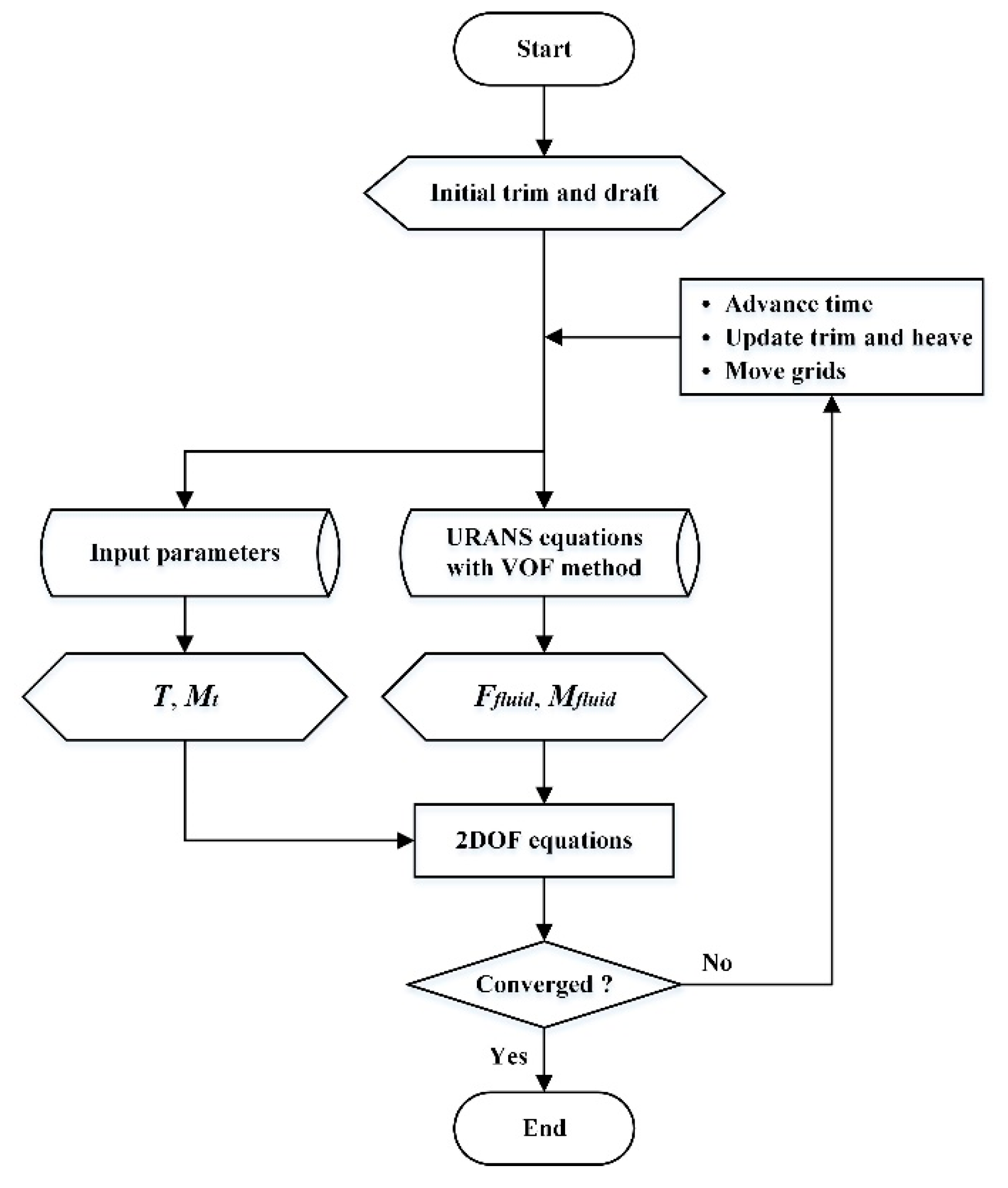
In summary, a brief workflow of the DFBI module is illustrated in Figure 3. The seaplane was released at initial trim angle and heave, then was free to trim and heave. For each time step, the aerodynamic and hydrodynamic forces acting on the seaplane were calculated by the URANS&VOF solver. The propeller thrust and moment were yielded based on data base and introduced into the DFBI model as external inputs. Then, the forces and moments were brought into Equations (8) and (9) to determine the vertical acceleration and pitching angular acceleration. Hence, the variations in heave and trim angle were yielded and the overset grids were relocated for the next time step. These procedures were repeated until the seaplane reached the equilibrium state.

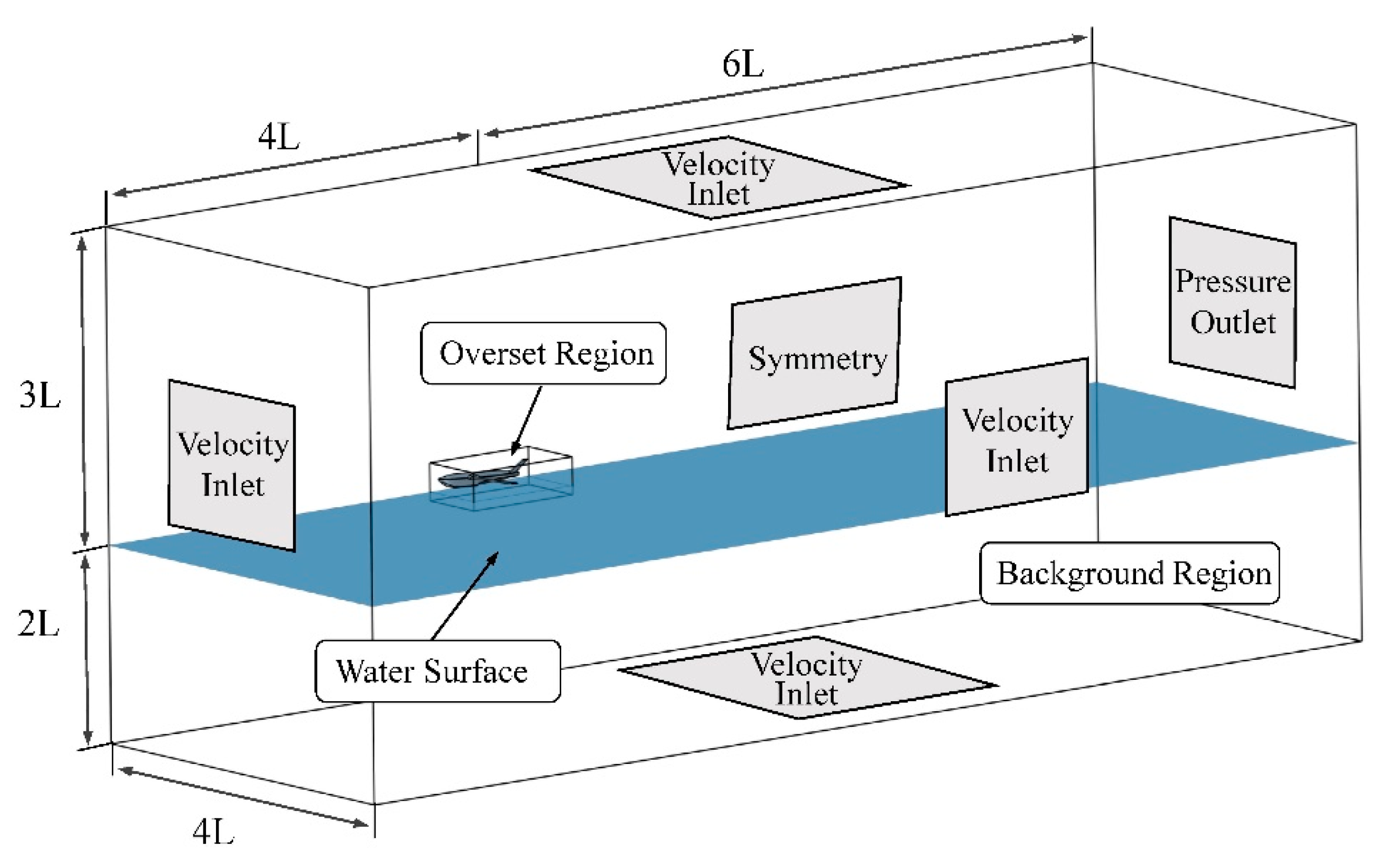
3.3. Computational Domain and Boundary Conditions

Overset mesh, also known as “Chimera” or overlapping mesh, was applied to move the grids with the dynamic seaplane for its accuracy, efficiency, and high-adaptability to the wide variations of trim and heave [16]. As for only the longitudinal performance was concerned, a half model with symmetry boundary was employed. The computational domain and boundary conditions are shown in Figure 4 where the dimensions are expressed in terms of the length of fuselage, L.

The computational domain combined a static background region and a moving overset region. The background enclosed the entire computational domain and the overset region moved with seaplane as a rigid body that ensured the grid quality near the seaplane. In the computational domain, the cells are grouped into active, inactive, or acceptor cells. At the overset boundary, the acceptor cells are used to couple the solutions on the two regions, and divide active and inactive cells in the background region. The discretized governing equations are solved within active cells which update with the moving overset region. A linear interpolation scheme was used for linking the solution between the background region and the overset region for its efficiency and accuracy [17].

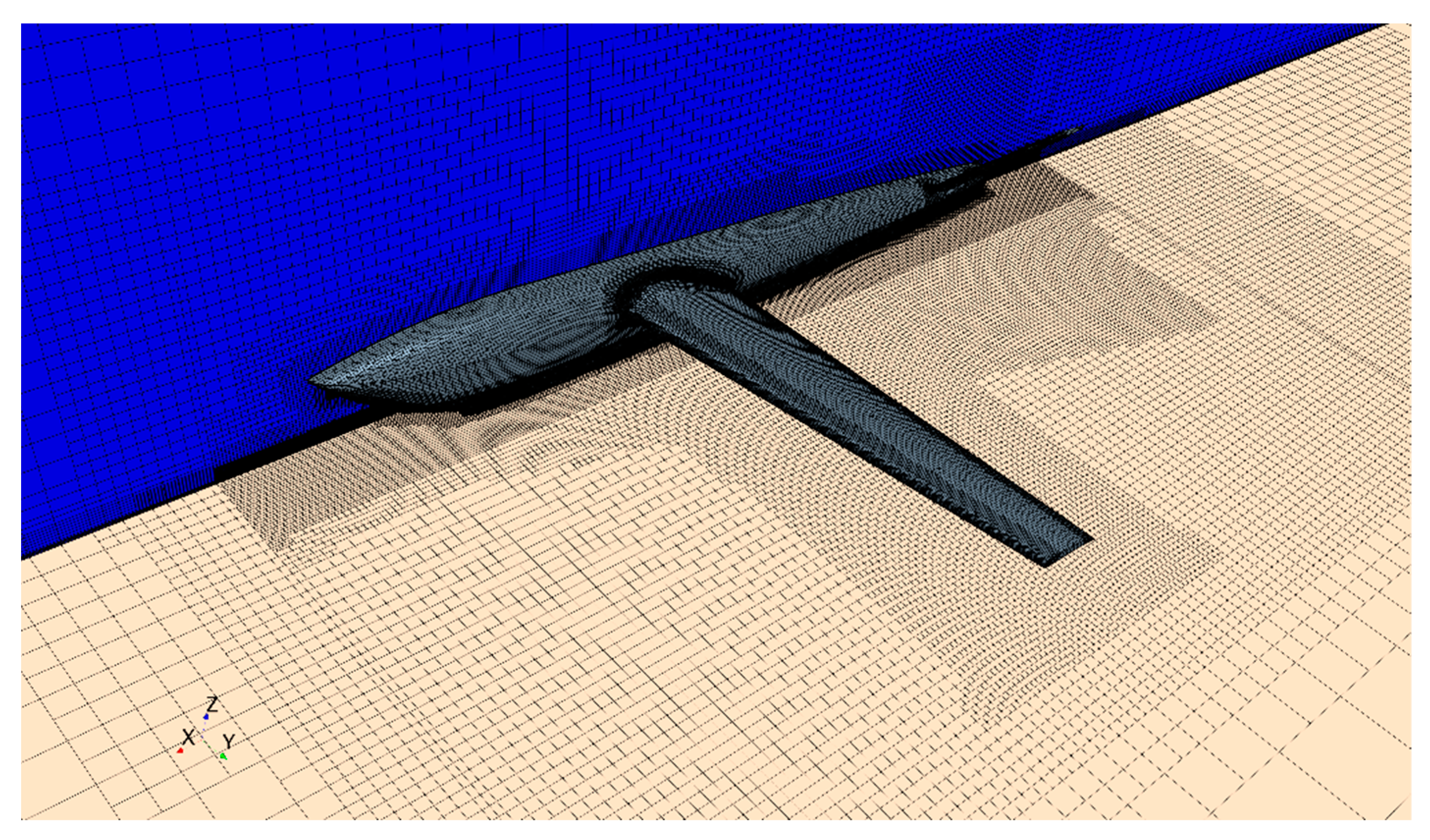
3.4. Grid Generation and Refinement

The grid design and topology and appropriate refinements were found crucial in obtaining reasonable results. Trimmed cell mesher was applied to provide high-quality hexahedral cells in both the regions due to the hexahedral cells aligned with the flow direction and interface making less numerical diffusion. For accurately describing the boundary layer flow, prism mesh with 10 layers and a stretching ratio of 1.2 was generated near the wall. The first layer was set to keep wall y+ in the range from 30–100 and All y+ Wall Treatment was utilized in all simulations.

Grid refinements were utilized for obtaining an accurate description of the flow field, particularly in the place where large flow gradient and complex flow occurred. Anisotropic hexahedral cells were used in grid refinements which allow specifying the cell size in each coordinate direction, which could achieve desired accuracy substantially reducing the number of grids in comparison with the isometric refinement approach. As demonstrated in Figure 5, besides the refinement in the air flow field, there were four refinement zones that are important for the description of water flow:

• The water surface zone. A sharp free surface is the precondition of accurate estimation of hydrodynamic performance. The grids located at water level should be well-refined to improve the resolution to capture the water surface. Note that a uniform cell height should be adopted at the free surface to avoid the smearing of the incoming water surface which is the mean source of numerical ventilation [18].
• The surrounding fuselage zone. In order to capture the complex flow near the hull, especially the spray flow at chine and the separation flow at step, the grids that encased the immersed surfaces of seaplane in the overset region were refined.
• The Kelvin wave zone. For capturing the Kelvin wave pattern induced by the seaplane, a triangular zone with a cusp angle of 39° was refined downstream of the seaplane. Otherwise, low-resolution grids would smear the wave patterns, resulting in an underestimation of wave resistance.
• The overlapping interface. A critical factor in successfully applying overset meshes is to have sufficient cells with uniform size and topology across the overlapping zone between background and overset regions. To improve the accuracy of interpolation, the overlapping interface in the background should be refined to match the size and the distribution of the grid at the interface of overset region, and the overlapping zone must contain at least 4–5 cell layers in both background and overset meshes.

3.5. Time Step and Iteration Number

Unsteady RANS equations were solved using implicit and iterative solver in order to find the field of all unknown quantities in each time step. The transient terms were discretized using 1st order temporal scheme. The time step used in the simulations was decided by two rules: First, in order to reduce the interpolation error at the overset interface, the time step should be limited to ensure the overset mesh moves less than half the smallest cell size relative to the overlapping zone within a time step. Second, the time step should satisfy the following equation:

$$\mathsf{\Delta }t=0.01~0.005L/V$$

(10)

Since a steady state is expected, increasing the number of iterations would bring little difference in final results. Weighting computational stability and efficiency, five iterations were applied in each time step. All simulations were performed in parallel using 24 Cores of Intel Xeon E5-2670 type CPU clocked at 2.3 GHz.

4. Validation Study

4.1. Validation with F6 Wing Body

The validation study towards aerodynamic analysis was performed based on the benchmark data of F6 wing body offered by Second AIAA Drag Prediction Workshop [19]. One of our main concerns of the aerodynamic simulation is the applicability of trimmed Cartesian mesh in describing the complicated air flow surrounding the wing. A grid refinement study was conducted using 3 systematic refined grids as demonstrated in Figure 6. The simulations were operated under the condition of $\mathrm{Ma}=0.75$, ${\mathrm{Re}=3\times 10}^6$, and lift coefficient of 0.5 to inspect the change in drag coefficient with the cells number. As shown in Figure 7, an increase in cells number has the effect of lowering the predicted drag coefficient values. The deviation between the numerical results and experimental data increased with increasing cell number, and the fine grid underpredicted the drag coefficient by 2.3%. Consequently, the numerical results of the trim grids were in accord with the ones of multiblock structured grids and unstructured tetrahedral grids.

Further, the medium grid with 4.28 million cells was simulated at the angle of attack ranging from −5–2 deg, corresponding to lift coefficient ranging from −0.1–6. The polar curves of numerical result and experimental data are compared in Figure 8. It can be seen that the numerical result are in good agreement with the experimental data with an average error in predicted drag coefficient of 2.81%, which satisfies the accuracy requirement of aerodynamic analysis.

4.2. Validation with Fridsam Hull

The validation study towards hydrodynamic analysis was carried out using the benchmark experiment of Fridsma. The Fridsma hull of load coefficient of 0.608, deadrise angle of 20 deg, and the length beam ratio of 4 was modeled for hydrodynamic simulations. The center of gravity of the hull is located 60% of length behind the bow in longitudinal and 29.4% of beam above the keel in vertical. The detailed geometry of the hull is shown in [20].

The girds with 1.9 million cells were generated following the rules reported in Section 3.4. The simulations were executed at five Froude number based on beam ranging from 0.59–1.78 to compare the resistance, trim, and sinkage with experimental data, Savitsky method, and previous numerical works of Mousaviraad [21] and O’Shea [22]. As shown in Figure 9, the model underestimated the trim with an average error of 6.5% in comparison with the experimental data. But at high Fr, the numerical error in trim is significantly smaller than the other numerical works. Besides, we accurately predicted the maximum trim at $\mathrm{Fr}=1.19$, which was not achieved by Savitsky and the other numerical works. The calculated results of $h/B$ matched the experimental data well, which was slightly underestimated at low Fr and over-predicted at high Fr. For resistance, we over-predicted the value at all Froude number with an average error of 8.2%. The error increased with speed which reaches the maximum 13.9% at a Froude number of 1.78. Frustratingly, the hump of resistance at Froude number of 0.89 shown in the experimental data was not predicted by any numerical method or Savitsky method. In sum, the numerical deviations of the dynamic two-phase flow solver are acceptable at the speeds ranging from the displacement to the planing stage. With the anisotropic refinements, our model used less efforts to achieve desired accuracy, particularly in trim prediction which is critical for the performance of a seaplane.

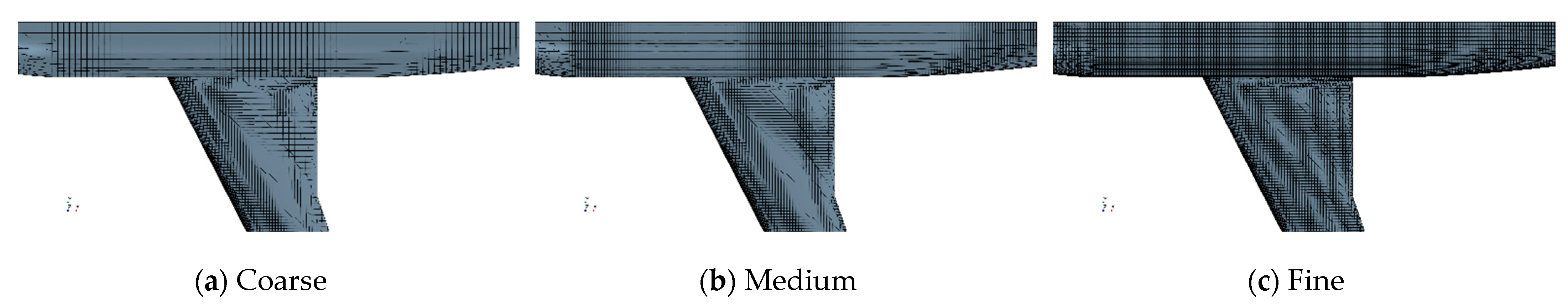
5. Results and Discussion

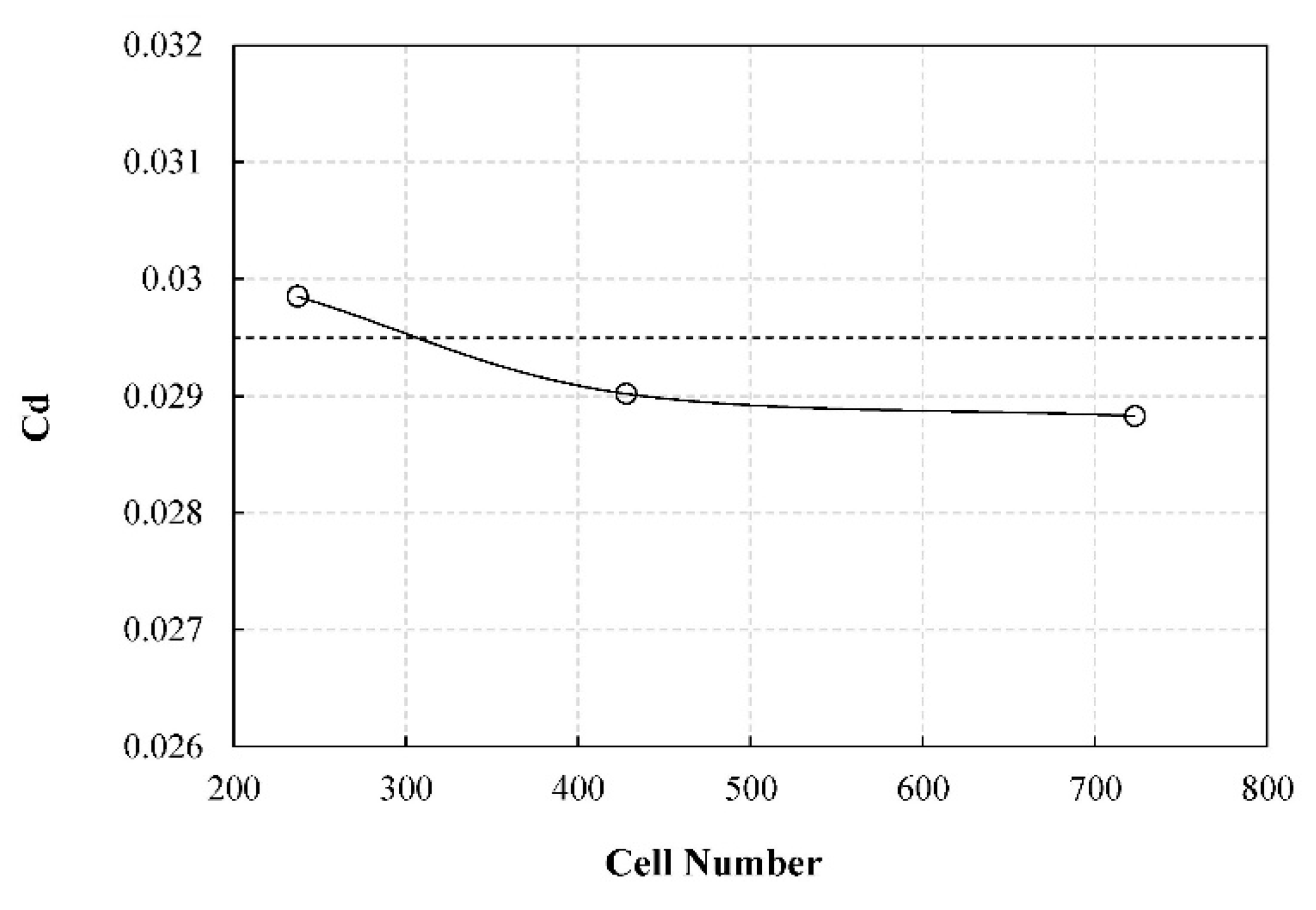
The grid of 6.5 million cells was generated for the simulations of the seaplane after a grid sensitivity analysis. The seaplane planning at twelve speeds ranging from 0 m/s to 14 m/s were simulated to examine the variations of heave and trim angle and their inherent relationship with aerodynamic performance and hydrodynamic performance. In particular, a detailed analysis of the resistance characteristics is performed. Additionally, a convergence study was performed to examine the influence of initial attitude and damping factors on the convergence time of 2DOF motion.

5.1. Heave

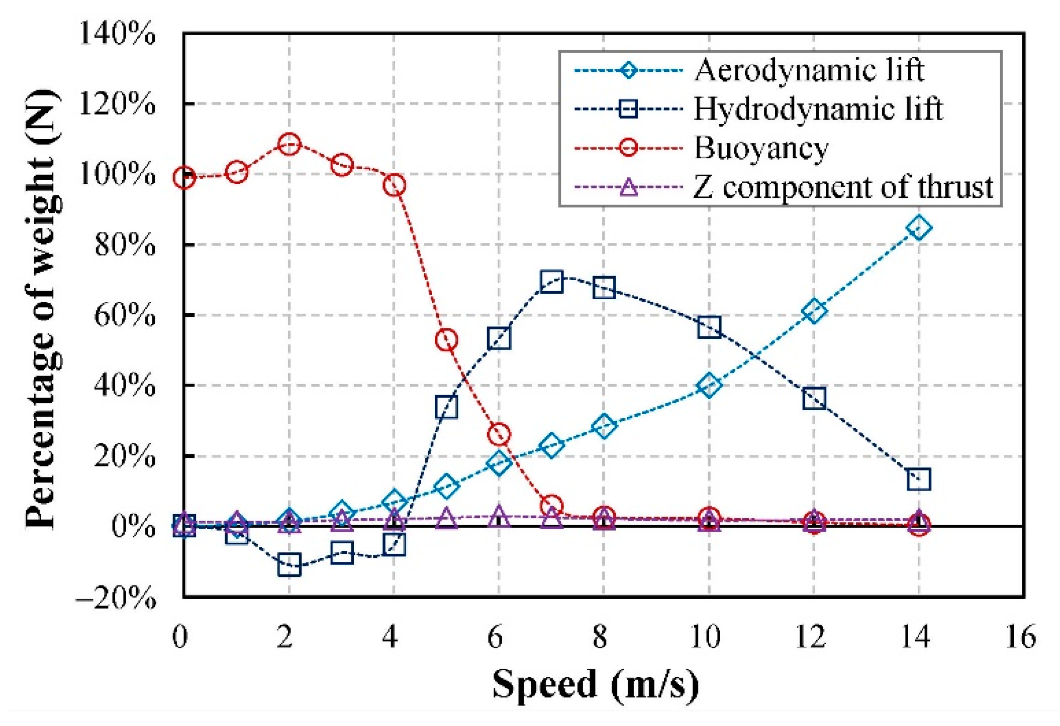
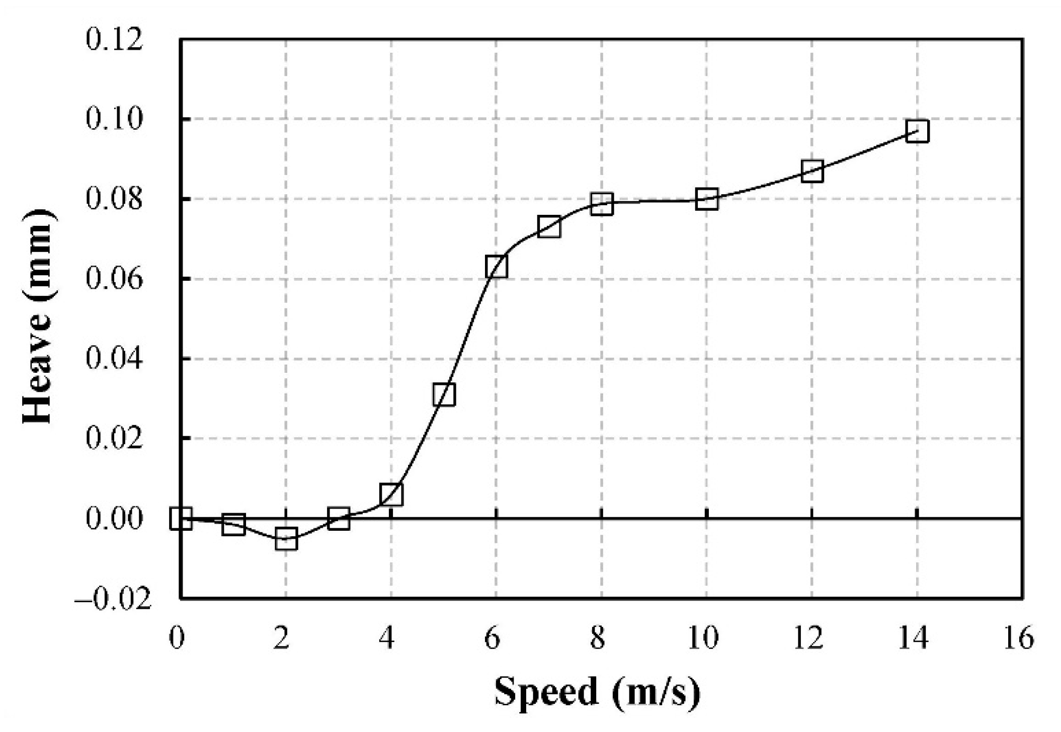
During the takeoff process, the seaplane is lifted by the aerodynamic lift acting on the wings and the buoyancy and hydrodynamic lift acting on the fuselage. The changes of buoyancy, aerodynamic lift, and hydrodynamic lift are shown in Figure 10. The heave of seaplane is essentially determined by the displacement volume of the fuselage that reflects the contribution of buoyancy.

In general, as the velocity increases, the increases of hydrodynamic lift and aerodynamic lift would reduce the contribution of buoyancy leading to an increase in heave as shown in Figure 11. While, it can be seen that the seaplane experienced a slight sinkage soon after the seaplane started moving. As indicated in Figure 10, at low speed regime the weight of the seaplane was mainly supported by buoyancy acting as a displacement hull. The forward motion of the seaplane caused a low pressure field on the bottom surface, creating a negative hydrodynamic lift that sucked the fuselage deeper into the water, known as squat effect.

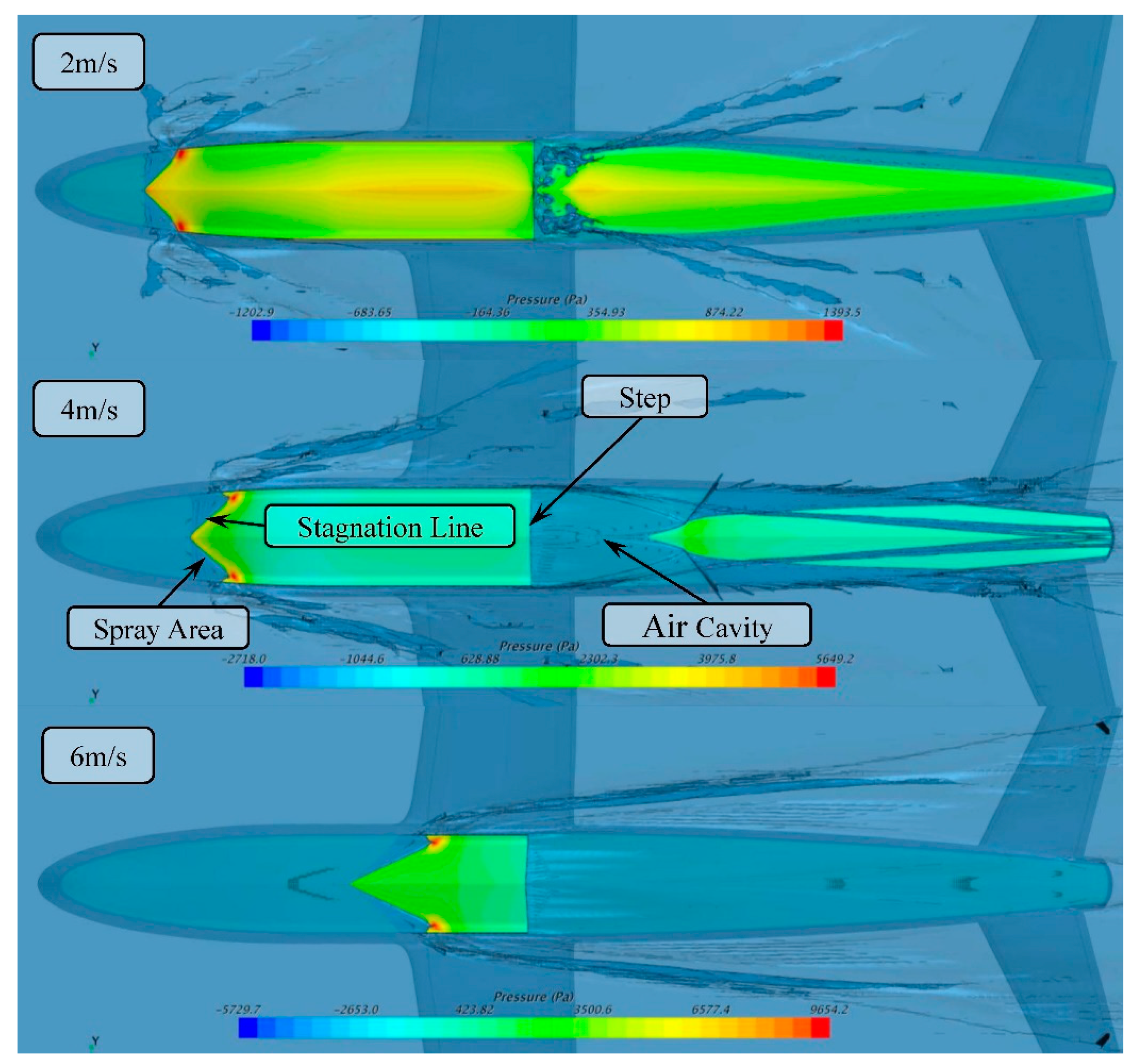
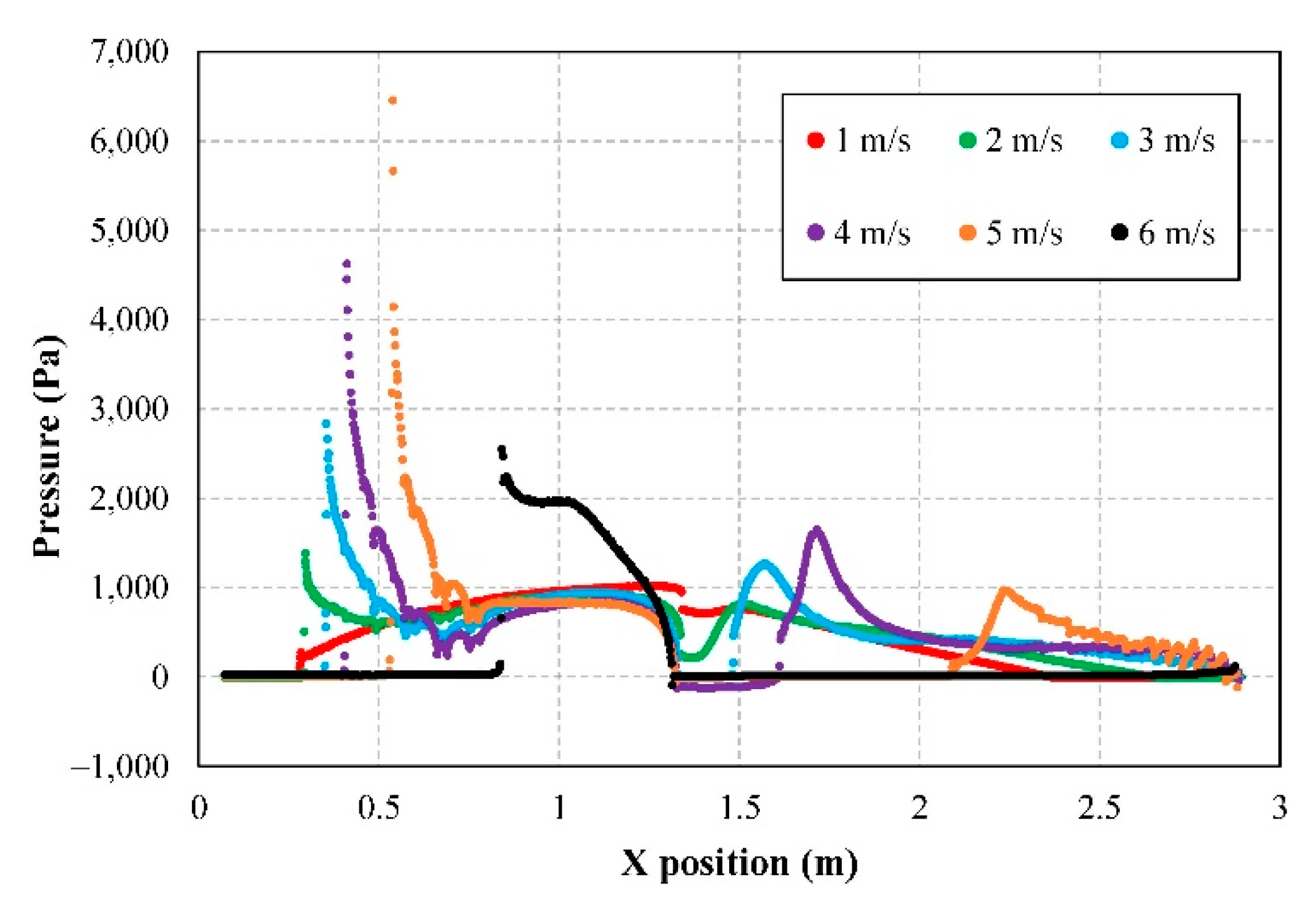
Figure 12 displays the disturbed water surface and pressure distribution at the bottom at speeds of 2 m/s, 4 m/s, and 6 m/s. It can be observed that the water interacted the fuselage at the stagnation line resulting in a pressure jump at the line. And part of the water rose up and blended into a thin sheet water flowing forward and outboard along the bow surface which is the source of spray. Figure 13 demonstrates pressure distribution along the keel line changes with speed. The peak of pressure at the stagnation line increased with speed, while slight decreases of pressure were observed behind the stagnation line. For the afterbody, the water separated at step and re-attached to the afterbody causing a second stagnation line which is apparently weaker than the one of forebody. After the speed of 4 m/s, the hydrodynamic lift increased rapidly and significantly heaved the seaplane. At high speeds, the heave further increased due to the growing aerodynamic lift.

5.2. Trim Angle

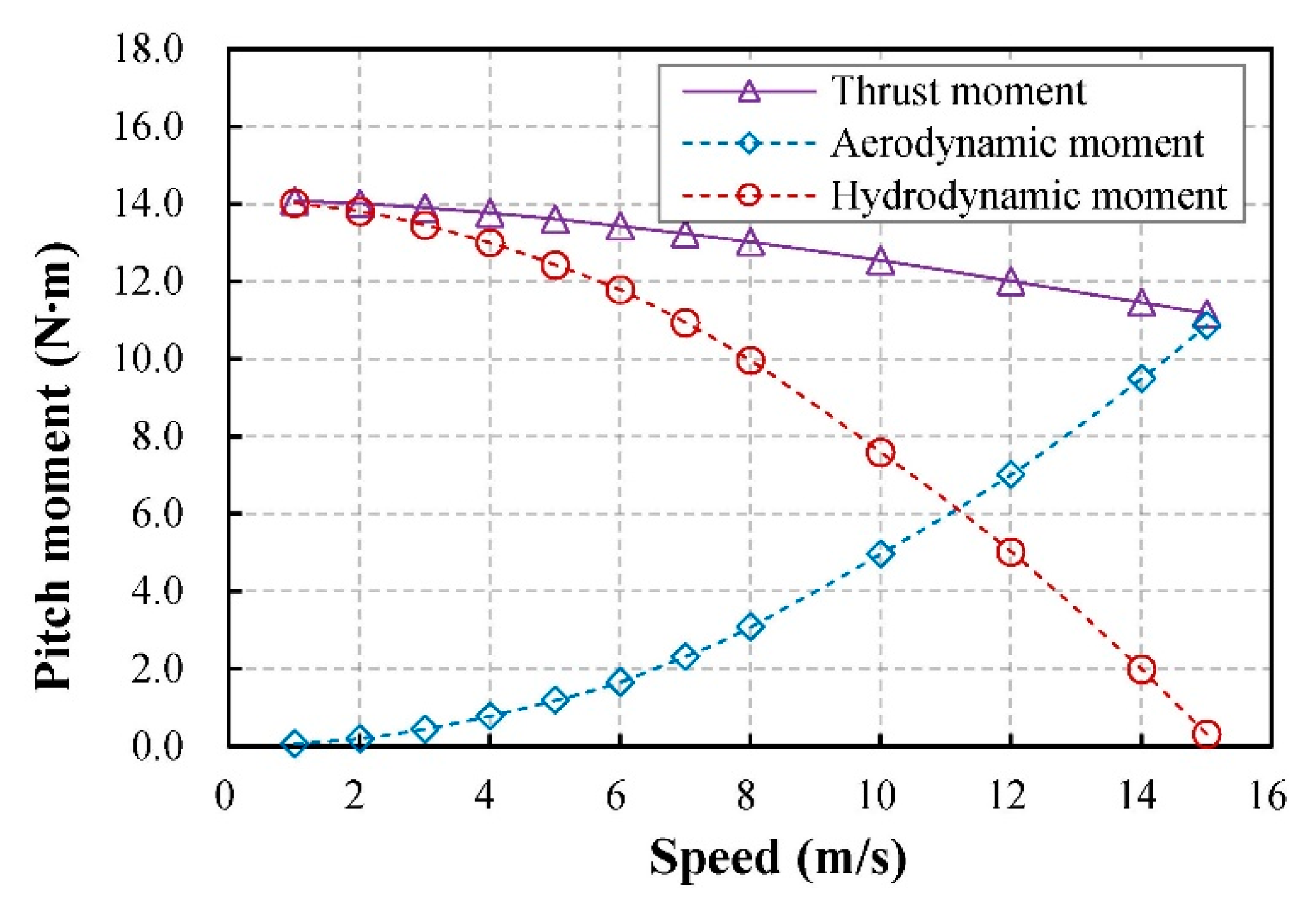
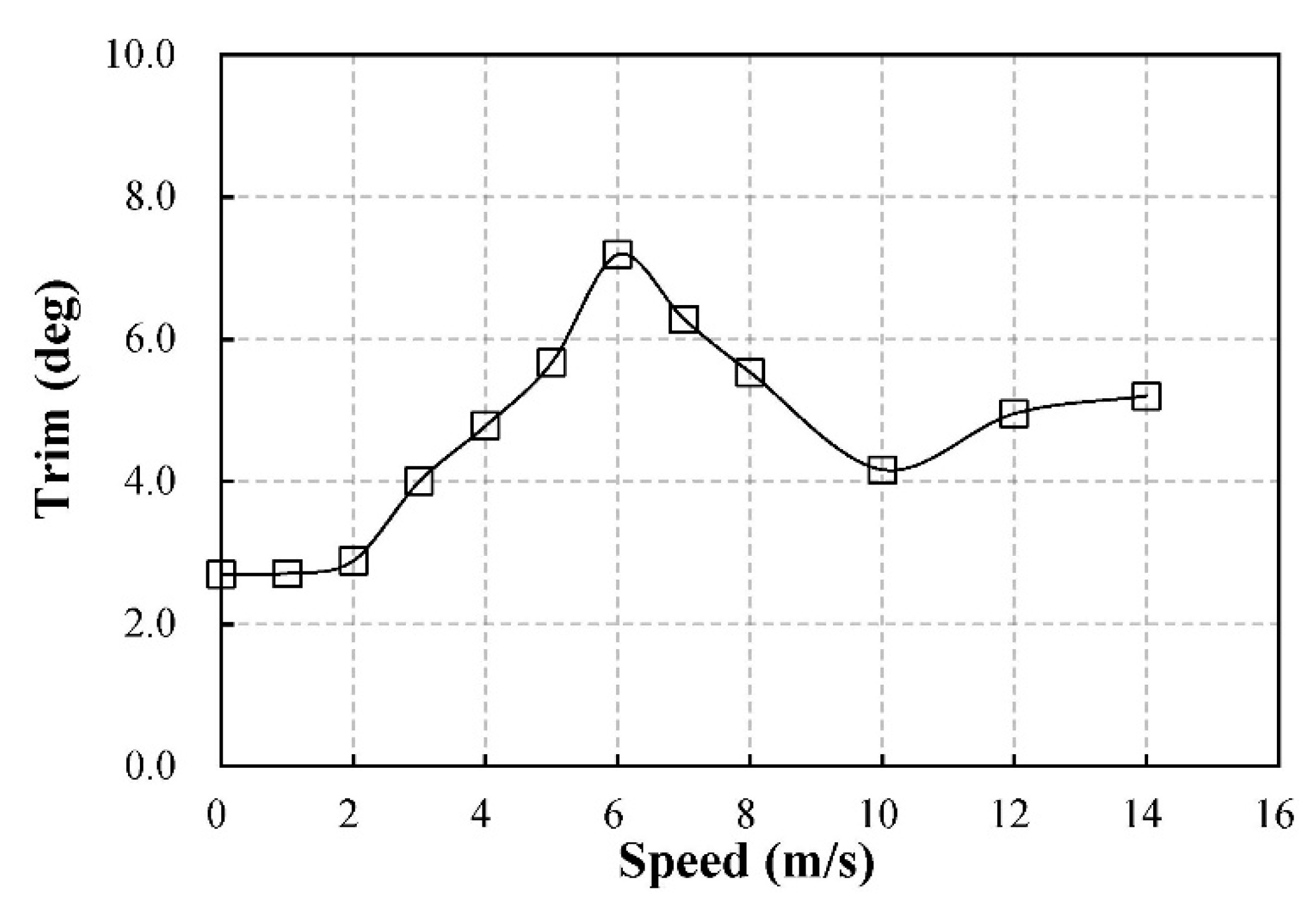
The trim angle plays an important role in both aerodynamic performance and hydrodynamic performance. Figure 14 shows the variation of pitching moments acting on CG produced by air, water and propeller thrust. And the trim curve against velocity is plotted in Figure 15. Since the propeller was high-mounted to avoid the water spray, it brought an unexpected bow-down pitching moment that lowered the trim angle. As illustrated in Figure 13, the increase of pressure at stagnation line moved the pressure center forward, creating a bow-up pitching moment that drove the trim angle to increase at low speed. Note that the maximum trim angle was limited by the afterbody, since the higher trim angle, the larger wetted surface area, and hence the stronger hydrodynamic bow-down pitching moment produced on the afterbody prevented further increase in trim angle. The trim angle reached the peak of 7 deg at a velocity of 6 m/s when the afterbody was nearly entirely unwetted.

Then, the seaplane started to plane on the single forebody. As the increasing hydrodynamic lift significantly reduced the displacement volume and wetted surface area of forebody, the pressure center moved backwards that decreased the trim angle. Moreover, as the water load reduced by the growing aerodynamic lift, it required a lower trim angle to create equal pitching moment by moving the pressure center forward. At high speeds, the aerodynamic pitching moment has been growing rapidly that it increased the trim angle preparing for a successful takeoff.

5.3. Resistance

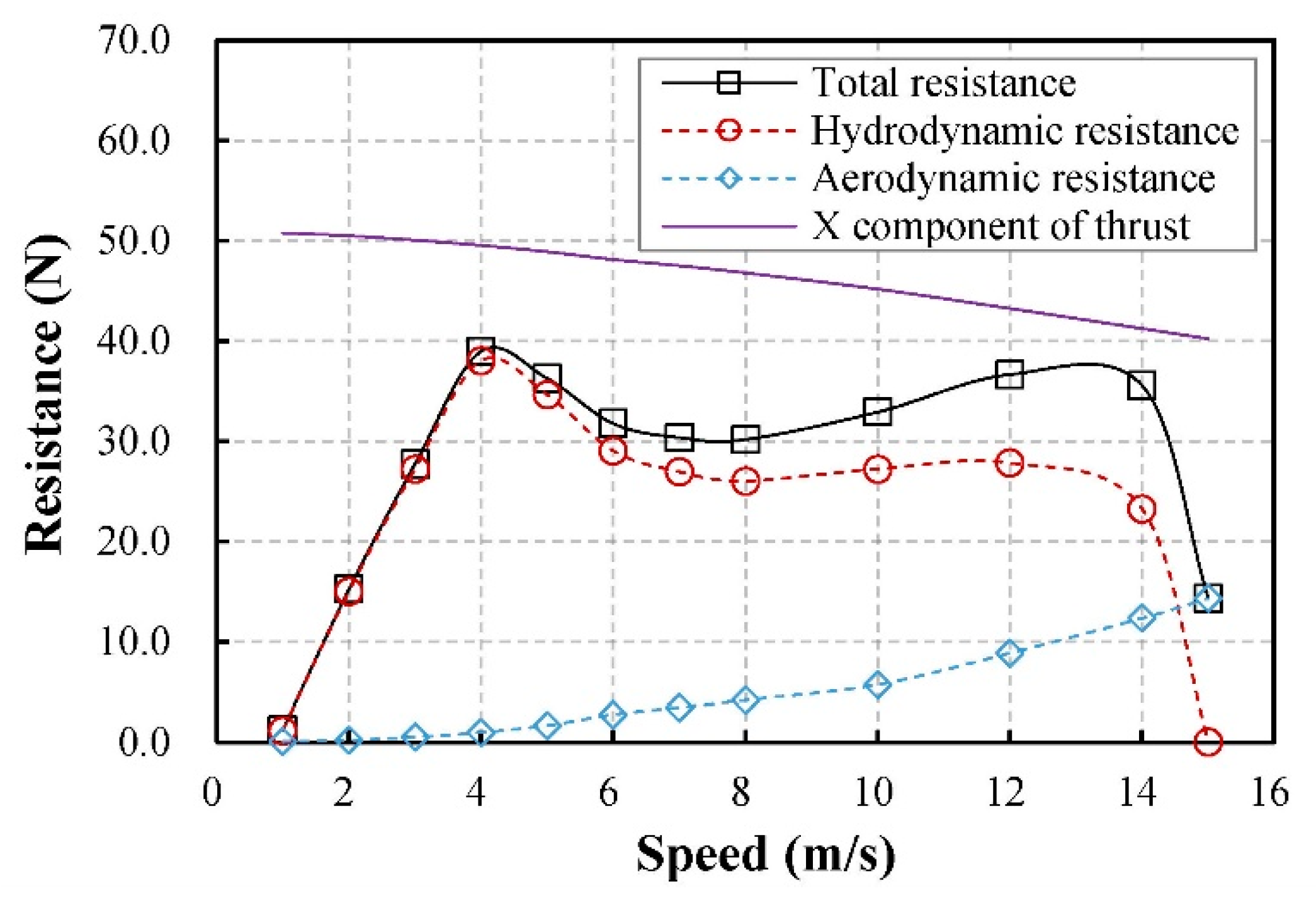
Resistance characteristics, including water resistance and air resistance, are the main concern of a seaplane design. Especially, the magnitude and corresponding speed of the resistance hump are critical in determining take-off performance and the requirement for propulsion. It can be seen from Figure 16 that there are two humps of total resistance: the first hump occurred at the speed of 4 m/s when the seaplane was transiting from the displacement to the planing stage, and the second hump occurred at the speed of 14 m/s around the corner of the takeoff. At the first hump, the hydrodynamic resistance contributed 97% of the total resistance and the residual thrust was about 15%. For the second hull, the hydrodynamic resistance contributed 65% of the total resistance while the residual thrust was only 7%. Since the propeller thrust decreased with speed, it is surprising to find that the second hump was a more critical point in a takeoff compared with the first hump, which was not concerned in previous studies [14,15].

As shown in Figure 16, it is no doubt that hydrodynamic resistance played the dominant role in total resistance. Next, the hydrodynamic resistance characteristics will be further analyzed. Based on the planing theory, the hydrodynamic resistance can be divided into the pressure component and friction component that fundamentally satisfy the relationship $R_w=△\tan \mathsf{\tau } + {0.5\mathsf{\rho }v}^2{S}_w{C}_f$. The pressure resistance, including the wave drag and viscous drag due to the separation of boundary layer, is proportional to the water load and trim angle. And the friction resistance could be evaluated with the dynamic pressure, wetted surface area, and skin friction coefficient.

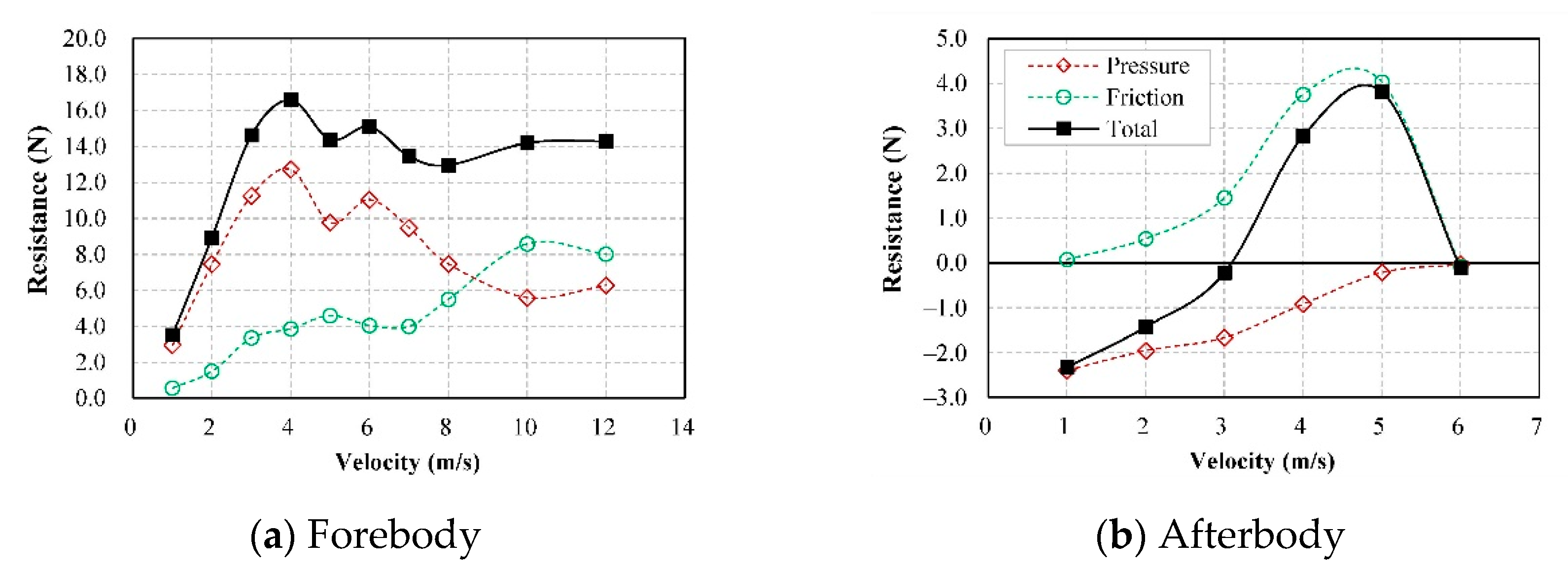
With CFD-post technique, the pressure component and friction component acting on forebody and afterbody could be calculated directly as shown in Figure 17. At low-speed regime, the main source of forebody pressure resistance was the generation of water waves at bow. Also, the water flow separating at step caused turbulence behind the step, which added to the pressure resistance. In theory, the pressure resistance is supposed to increase as the trim rises with speed. Surprisingly, we noticed that the pressure resistance started to decrease at a velocity of 5 m/s when the trim angle was still rising. This phenomenon is related to the convex surface of the fuselage. At low speeds, the water surface encountered with the convex bow making the local trim angle of the stagnation line higher than the trim angle measured from the keel, which produced a larger backward component of pressure force that increased the resistance. As the seaplane heaved, the stagnation line moved backward to the straight section, and the local trim angle has been reduced, resulting in the decrease of the pressure resistance. 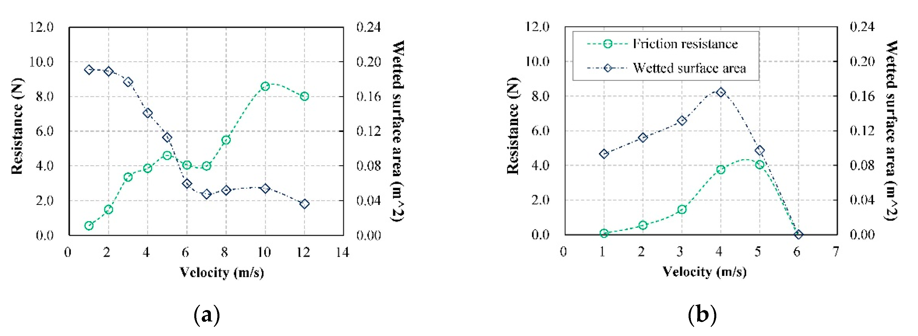It can be seen from the Figure 18a that the wetted surface area of forebody gradually decreased that limited the increase of friction resistance. Additionally, we found the reversed flow in the spray area provided a forward shear force that could slightly decrease the overall friction resistance.

For the afterbody, due to the upward stern, the pressure acting on the afterbody always provided a forward component that reduced the total hydrodynamic resistance. Since the fuselage is narrower toward the stern, the afterbody sinked farther into the water as the trim increased, significantly increasing the wetted surface area and afterbody friction resistance. Taken together, the increase of pressure resistance at forebody and friction resistance at afterbody determined that the total hydrodynamic resistance reached the first hump at the velocity of 4 m/s.

At rest, the step was entirely submerged under the water surface. As shown in Figure 12, with the water flowing over the step, the low-pressure region formed behind the step essentially forced the water surface to sag and allowed air to be sucked in. Air proceeded downward along the step from the chine to the keel until the step was completely ventilated at a velocity of 3 m/s. Then, the afterbody acted as an additional planing surface in the disturbed wake of the forebody. The water separating from the step and re-attached to the afterbody created an air-filled cavity that reduced the wetted surface area of the afterbody. The air cavity kept extending towards the stern until the afterbody entirely got out of the water at a velocity of 6 m/s.

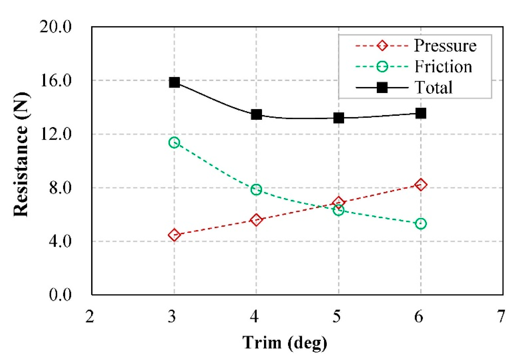
Since then, the seaplane has been planing with the single forebody. As shown in Figure 18, the wetted surface area slightly grew with speed, while the friction resistance increased rapidly and overtakook the pressure resistance to become the major source of hydrodynamic resistance. Moreover, the results showed that the hydrodynamic resistance characteristics were sensitive to the change of trim angle. The hydrodynamic resistance characteristics of fixed trim angles ranging from 3–6 deg at a velocity of 10 m/s are plotted in Figure 19. Since the wetted surface area varies inversely with an exponential power of trim [9], the friction resistance increased rapidly as the trim angle decreased. Whereas, the pressure resistance increased linearly with the trim angle. Hence, there is an optimum trim angle that minimizes the sum of pressure and friction components for each speed. To avoid the substantial hydrodynamic resistance at the second hump, the trim angle should be close to the optimum trim angle.

However, it is difficult to operate the seaplane to plane with the optimum trim angle at each moment during the takeoff to achieve the optimum takeoff performance. As shown in Figure 19, actually the hydrodynamic resistance increased slowly in a range within 2 deg around the optimum trim angle. Hence, it is more practical to operate the seaplane planning at trim angle within the optimum range, typically between 4–6 deg, to achieve a satisfied takeoff performance.

5.4. Convergence Study

Another purpose of this paper is to analyze the factors that determine the convergence time of the 2DOF motion. It is time-consuming to wait for the 2DOF motion to reach the equilibrium state, especially for the simulations with millions of cells. Setting a proper initial attitude or adding additional damping terms into the rigid motion equations are considered as an efficient way to save convergence time [23], but have not been verified with a systematic study. Therefore, a convergence study was performed to discuss the influence of initial attitude and damping terms on the convergence time through a series of simulations at a velocity of 5 m/s.

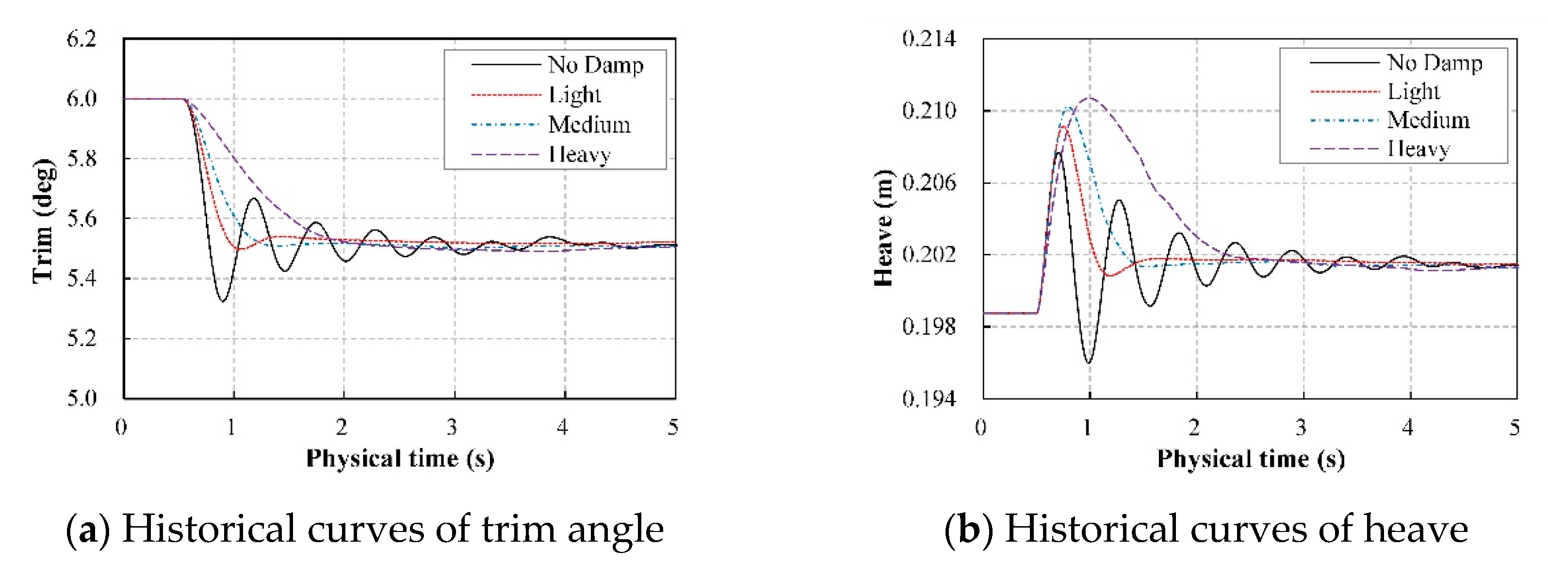
First, different damp factors were introduced into the 2DOF equations, and the historical curves of trim and heave are compared in Figure 20. It can be seen that the damping force and moment observably weaken the excessive oscillation and reduce the convergence time. But the stronger the damping factors, the longer the oscillatory period. We recommend that the damp factor should be decided to ensure that one oscillatory period could be observed in the historical curve.

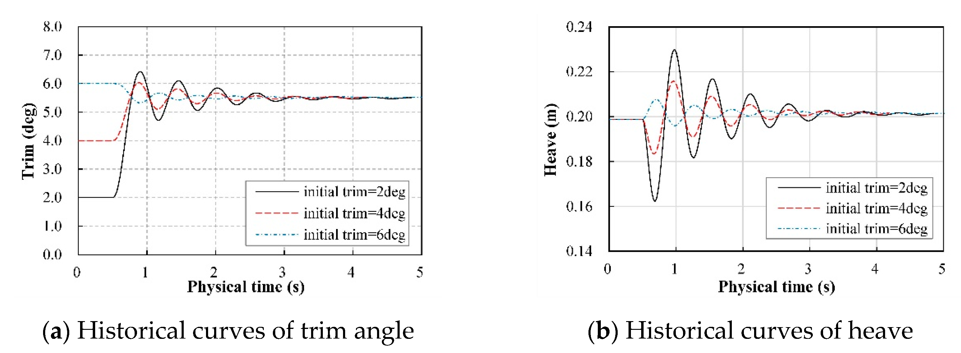
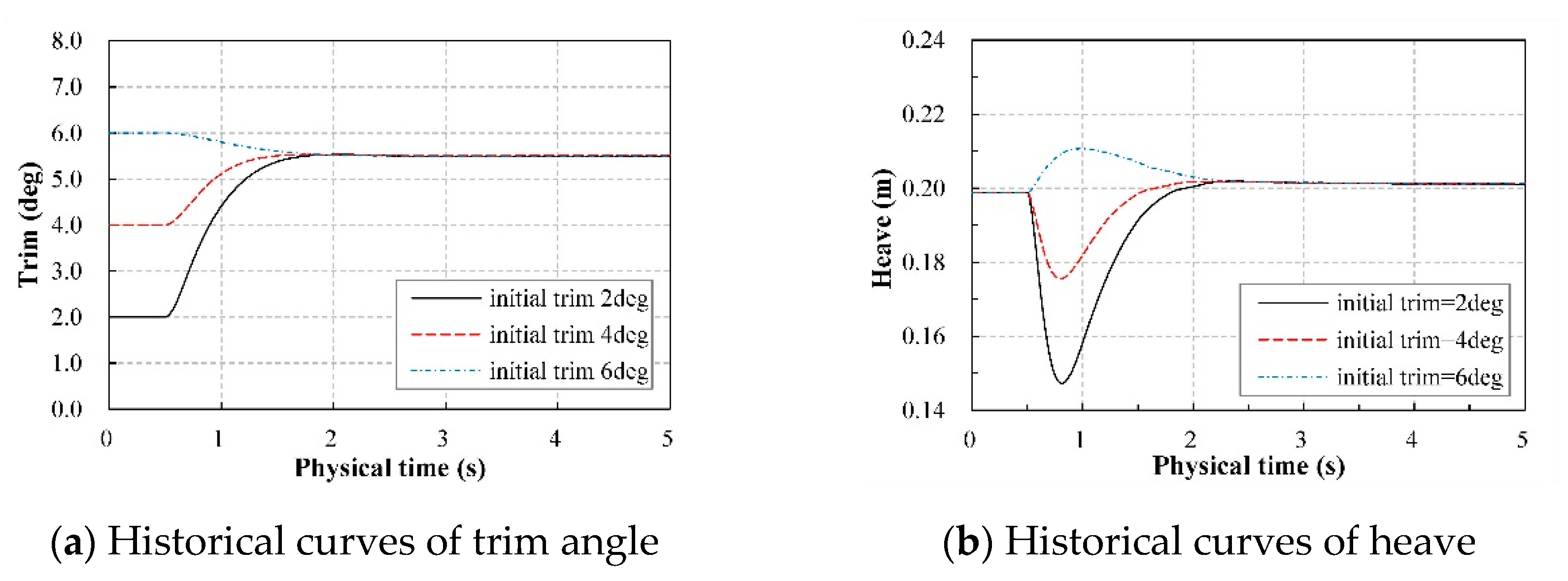
Then, the influence of the initial attitude was investigated by releasing the hull at the different trim angles of 2 deg, 4 deg, and 6 deg, respectively. As demonstrated in Figure 21, the difference between the initial trim angle and the final equilibrium trim angle decides the amplitude of oscillation, but barely affects the convergence time. But when damping terms were added, the free motions were all converged within one period and little difference in convergence time is observed in Figure 22. In conclusion, for a dynamic motion ending with a stable state, adding damping terms is the most effective way to accelerate the convergence regardless of the initial attitude, which could save more than 50% physical time.

6. Conclusions

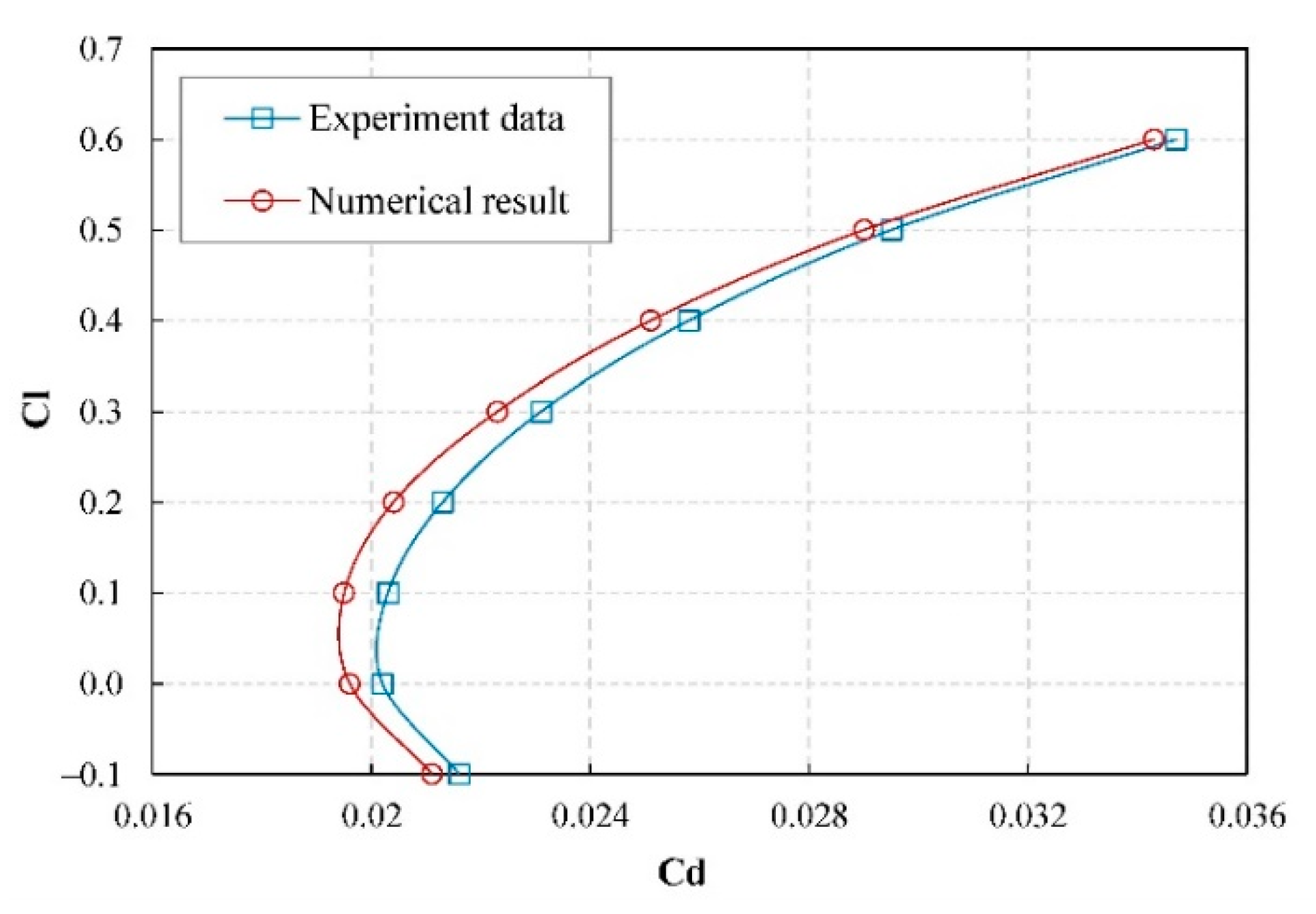
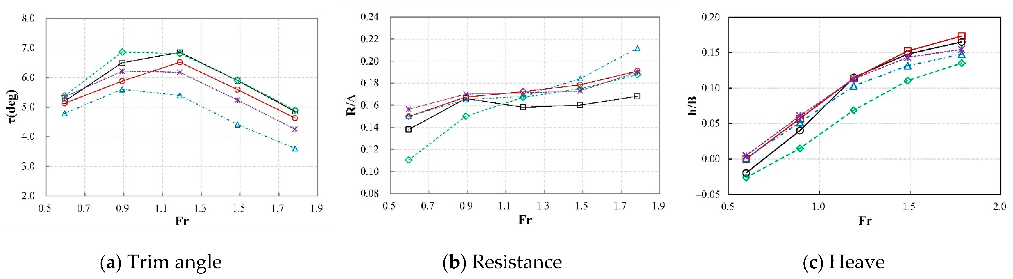
This paper aims to investigate the take-off performance of a seaplane by numerically modeling the air-water two-phase flow around a seaplane using RANS equations with VOF method. In order to determine the equilibrium trim angle and heave of the seaplane at different speeds, the free motion in trim and heave in response to aerodynamic forces, hydrodynamic forces, hydrostatic forces, and propeller thrust was realized by DFBI module and overset mesh technique. The numerical model was validated based on the benchmark model of the F6 wing body and the Fridsam hull.

The seaplane planning at speeds ranging from the standstill to the takeoff were simulated. Based on the numerical results, we investigated the variations of heave and trim angle and their inherent relationship with the aerodynamic performance and hydrodynamic performance. The results prove that hydrodynamic performance plays a dominant role in governing the take-off performance, and the hydrodynamic performance was essentially determined by the pressure distribution and the location of the stagnation line. Besides, the results turned out that heave could be treated as a main parameter that reflects the contribution of buoyancy.

The resistance characteristics are the main concern in this study. There are two humps of total resistance: the first hump occurred at the transition from displacement to planing, and the second hump happened at the high speed planing stage near the takeoff. The results show the hydrodynamic resistance contributed nearly all of the resistance at the first hump. And the increase of pressure resistance at forebody and friction resistance at afterbody were the major causes of the first hump of hydrodynamic resistance. We considered that the stagnation line located at convex surface at bow created a backward pressure component that considerably increased the pressure resistance at forebody. And the increase of friction resistance at afterbody is related to the afterbody sinking farther into the water as the trim increased. Furthermore, we found that the hydrodynamic resistance at high speed was significantly affected by the trim angle. The trim angel of a seaplane should be operated in an optimum trim range, typical between 4–6 deg, to minimize the hydrodynamic resistance. Otherwise, the hydrodynamic resistance would significantly increase as the trim angle deviates from the optimum trim range, resulting in a substantial second hump of resistance. Note that as the propeller thrust decreased with speed, more attention should be paid to the second hump of which the residual thrust might be less than the one at the first hump.

The convergence study concludes that the utilization of damping terms is the most effective way to accelerate the convergence of the 2DOF motion ending with a quasi-static state, while the offset between the initial trim angle and the final equilibrium trim angle only decides the amplitude of oscillation but barely affect the convergence time.

This paper provides a numerical approach to predict the resistance and attitude of a seaplane taking off in calm water. The investigation on take-off performance gives a better understanding of the variation of aerodynamic performance, hydrodynamic performance, and hydrostatic performance during the takeoff, which would provide some guidance in the integrated design of aerodynamics and hydrodynamics of the seaplanes.