1. Introduction
Approximately every two years the number of transistors in a classical microprocessor doubles [
1]. As a result, transistors are becoming smaller and require lower voltages to operate. However, current classical computers are reaching the limit of computational capacity because when manipulated in circuits of such small size, electrons tend to act unpredictably. They can also pass through the walls of conduction channels in what is known as the ‘tunnel effect’ [
2]. One of the alternatives to classical computing is the exploitation of the laws of quantum mechanics in computational environments.
Quantum computing is the development of computational technologies that are based on the laws of quantum mechanics. This type of computing enables the creation of systems to store, process, and transfer information encoded in quantum media. The first idea of a quantum computer was proposed in 1982 [
3] and was based on the first classical computing machine defined by Alan Turing [
4]. The Turing machine manipulated symbols on a strip according to a table of rules that simulated a computational algorithm. The first proposal for quantum computation replaced the strip with a sequence of two-state quantum systems. The machine evolved in steps. At the end of each step, the tape was always in a fundamental state of ‘1’ or ‘0’. However, during each step, the machine could be in a superposition of spin states.
Soon after the first idea for a quantum computer, some scholars [
5] introduced the ‘speculative’ idea that a computer based on the laws of quantum mechanics could perform complex calculations faster than conventional binary computers.
Conventional computers convert data into a series of binary digits called bits that constitute the basic units of information. These bits can only have the values of ‘0’ and ‘1’ and are encoded in integrated circuits according to electrical signals of different voltages. Technological advancements have enabled the creation of devices that act as bits. Today an integrated circuit contains millions and millions of transistors.
In contrast, data processed by quantum computers use ‘qubits’ that can have the value of ‘0’ and ‘1’ at the same time. Unlike bits, qubits can be in a superposition of both states [
6].
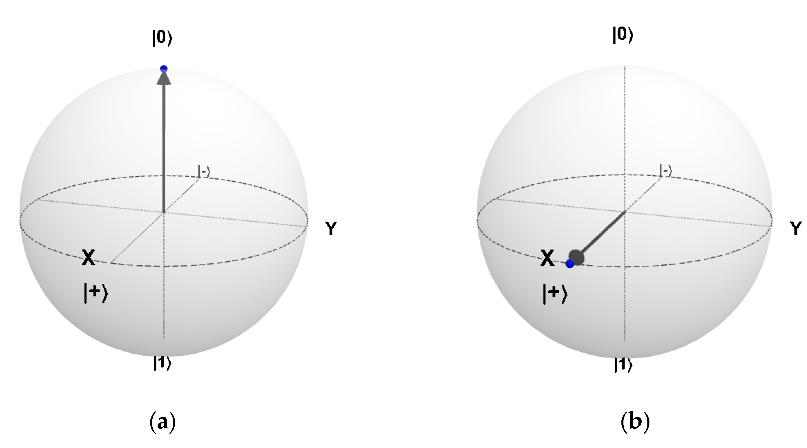
The Bloch sphere [
7] is a geometrical representation of all possible superposition states that a qubit can adopt, as can be seen in
Figure 1a. Each point on the surface of the sphere corresponds to a pure state of the Hilbert space of complex dimension 2. The point of coordinates (0,0,1) corresponds to an eigenvector with a positive eigenvalue of the Pauli matrix and the point of coordinates (0,0,−1) corresponds to the eigenvector with negative eigenvalue. Both states are expressed with the notation |0〉 and |1〉 and correspond to spin up and spin down. The qubit can be represented as a linear combination of both states, as shown in the equation, where a and b are complex numbers, and where |
α|
2 + |
β|
2 = 1.
The Bloch sphere makes it possible to visualize the action of different quantum gates graphically. For example, one of the most used quantum gates is the Hadamard gate that operates on a single qubit. This gate is equivalent to the combination of two rotations, one of pi about the z-axis followed by a rotation of pi/2 about the y-axis of the Bloch sphere as shown in
Figure 1b.
The Hadamard gate is the ‘quantum Fourier transform’ performed on a qubit [
8]. The Hadamard gate is usually the first stage in a quantum circuit because it places the qubit in a state of superposition. However, the Bloch sphere model, while conceptually determining the states that a qubit can have, has the major limitation of not being useful for showing the ‘entanglement’ of several qubits. One of the most important advantages of state superposition is that, while with n bits one can encode a single state out of
2n possible states, with n qubits one could encode
2n states simultaneously. This can be achieved by taking advantage of the possibility of rotation of the qubit values. Given this, quantum computers can dramatically increase the capacity of storage devices by storing huge amounts of data in a very little space [
9].
In addition to superposition, qubits share another principle of quantum physics called entanglement [
10]. If superposition is the qubit’s characteristic of being in several states at the same time, entanglement is the correlation that exists between two qubits, even if they are not physically in the same place. When quantum entanglement occurs between two particles, their quantum states are determined as if they were a single particle. Therefore, any variation in the quantum state in one of them instantaneously causes the same variation in the other particle. As previously stated, the quantum state of n qubits implies the superposition of all possible configurations (
2n). The quantum entanglement between the electron spins of n qubits exponentially increases the Hilbert space from
2n to
2n dimensions.
2. Quantum Technology Approaches
Although there is a technological challenge for the development of quantum computers, the theoretical framework on which they are based is solid and well defined. It allows all the possibilities that classical computing offers and far more. From a strictly mathematical point of view, the operations performed with qubits can be expressed with matrix algebra, tensor products and probability calculations, to name but a few concepts central to the discipline.
However, creating physical devices that behave in line with quantum mechanics has been a technological challenge; a challenge that has led several companies to invest heavily to achieve ‘quantum supremacy’ [
11]. A variety of technologies exists to implement quantum devices.
2.1. Superconducting Circuits
One type of technology used to generate qubits is based on superconduction. These circuits are characterized by the use of qubits that can be selectively introduced or removed. Superconduction circuits can take several different architectures. For instance, superconduction-based qubits can be designed by the interconnection of superconducting electrodes with Josephson junctions. The system is based on the capacitive contribution of the Cooper pairs as well as on the inductive contribution of the jump between two electrodes [
12]. Some examples of qubits based on these concepts are the charge qubit, the flux qubit, the phase qubit, and the fluxonium. The transmon (“transmission line shunted plasma oscillation qubit” [
12]) is a type of superconducting charge qubit that was developed in 2007 to reduce sensitivity to noise. This technology is based on a multilevel system, used as qubits if all their dynamics are confined to two quantum levels. The parameters of a qubit cannot be perfectly obtained during its fabrication process, despite knowing its Hamiltonian capacity [
13]. At present there is still a high discrepancy between two fabricated qubits. Superconducting qubits typically operate roughly in the range between 4 GHz and 8 GHz, an energy range that gives rise to the states of 0 and 1. Despite the complexity of superconduction circuits, control of the qubit entanglement is achieved by changing the direction of the circuit current corresponding to the 0 and 1 states [
14].
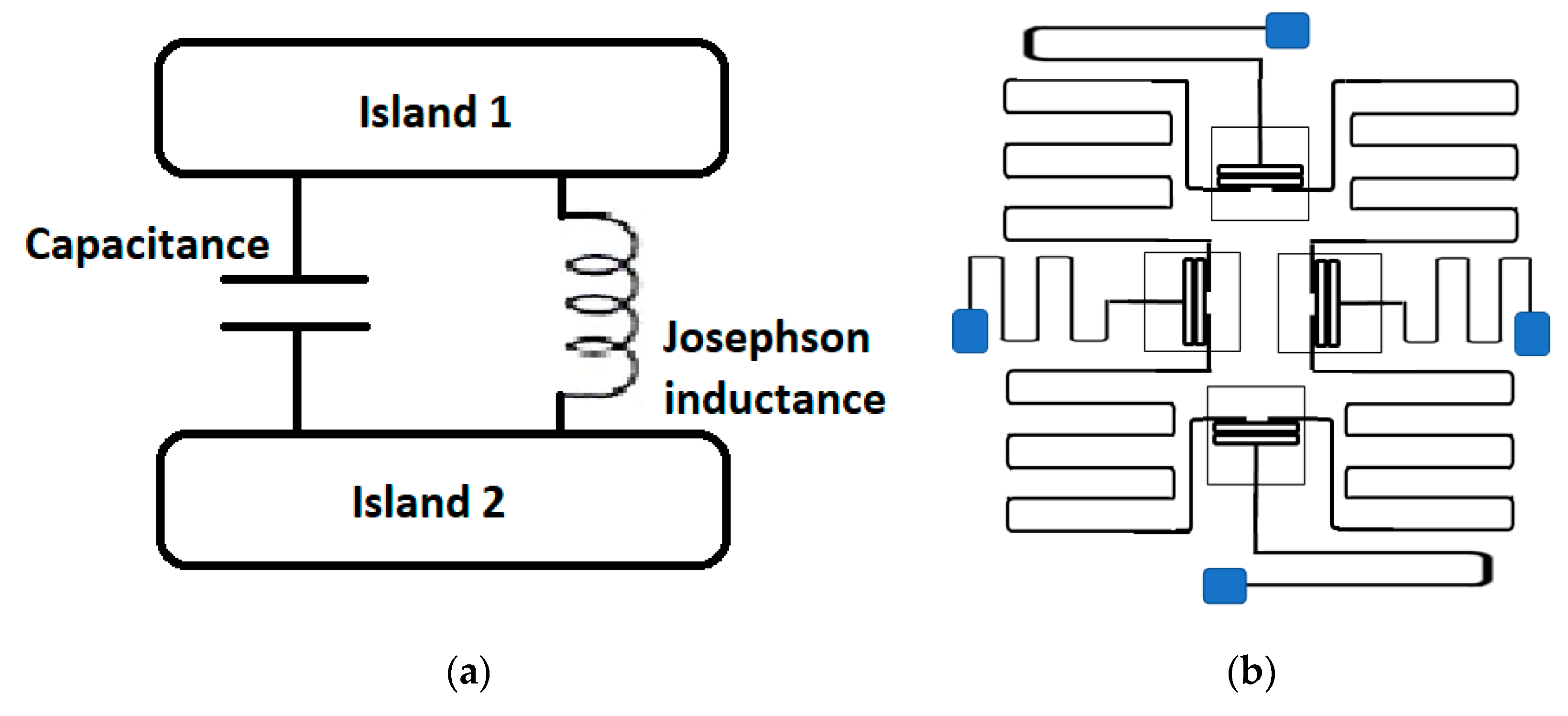
The transmon consists of two islands connected by a capacitor and a Josephson inductance. In other words, its operation is based on an LC oscillator. The use of a Josephson inductance provides inductive energy in the form of a cosine function. Consequently, the transition of the transmon from the first to the second excitement state is less than 300 MHz. In practice, this difference is sufficient to confine the dynamics to a subspace of two qubits using pulses of a duration of about 20 ns. For two-qubit quantum gates, two inductances in parallel are needed.
Figure 2 shows the structure of a transmon and the implementation of a quantum superconducting device.
For this implementation, the quantum chip must be completely isolated and at a temperature of only a few tens of millikelvins above absolute zero. To achieve such low temperatures, cryogenic technologies are required. Therefore, a quantum computer requires the use of thermal insulators to prevent noise that would compromise the quality of the qubit. So far, due to the state-of-the-art technologies requiring a high investment, only a few companies such as Google, IBM, Rigetti, Intel, and Alibaba have ventured into developing quantum computers based on superconducting circuits.
2.2. Ion Traps
Another technology is ‘ion traps’. Ion traps are electromagnetic and optical fields used to trap electrically charged individual atoms, i.e., ions [
15]. These ions are pushed by their vibrations to entangle their spin states. Ion traps also require operating temperatures close to absolute zero in order to achieve better control of the quantum states of the ion. This is done by decreasing the atom’s vibrational energy, thus exciting the atom to increase its internal energy and thereby transferring the quantum superposition of the electronic states to vibrational modes. In short, qubits are stored in the internal states of ions. The resulting electron detraction causes the ions to interact with each other through electromagnetic fields [
16].
For any quantum operation, however basic, sequences of several pulses are required to minimize perturbation or decay as much as possible. In addition, the applied magnetic fields and laser sources are required to be very stable [
17]. Organizations such as IonQ and the Massachusetts Institute of Technology are advancing the development of quantum computers using this technology [
18].
2.3. Majorana Quasiparticles
Fermions are quasiparticles that have been theoretically defined to form excitations in superconductors [
19]. Majorana fermions are particles that correspond identically to their antiparticles. Indium antimonide nanowires can be used to create qubits in this way. The production of Majorana fermions in the laboratory is an arduous task that requires the combination of the latest advances in nanotechnology, superconductivity, and material sciences. First, a crystal nanowire consisting of a 100-nanometer-long column of atoms is constructed. The wire is then connected to a circuit capable of measuring single electrons passing through it. Theoretically, if all the electrons in the wire are magnetized, fermions emerge from both ends of the wire.
The bond that exists between each pair of Majorana particles could be exploited to store quantum information in two different intertwined locations. This duplicity and the greater theoretical stability of these fermions could result in qubits that are more stable and less sensitive to local ambient noise. While a study partly funded by Microsoft claimed to have detected Majorana fermions [
20], its authors themselves retracted the claim. There are also several subsequent studies that cast doubt on the detection of these quasiparticles [
21]. The main advantage of this technology with respect to superconductors that store data in a single object is the possibility of a qubit encoding a single bit of information in several fermions. The qubit remembers whether it has moved clockwise or counterclockwise.
2.4. Spin Qubits
Quantum computers based on spin qubit technology operate by controlling the spin of electrons and electron holes in semiconductors [
22]. The Loss–DiVicenzo quantum computer is the first quantum computer built employing this technology [
23].
The Loss–DiVicenzo quantum computer works in the half-spin degree of freedom of individual electrons confined in quantum dots. Quantum dots are semiconductor nanostructures that confine the motion of electrons in all three spatial directions and were discovered in 1981 [
24].
The Fermi gas model, an ideal free fermion system in which electrons do not interact with each other, is used to operate the Loss–DiVicenzo quantum computer. Two-dimensional electron gases are introduced in semiconductors such as gallium arsenide [
25], silicon [
26], germanium [
27] and graphene [
28].
Spin qubits require slightly higher operating temperatures than superconducting qubits, namely 1 kelvin at 20 millikelvins, a factor than can potentially reduce system complexity. Another apparent advantage is that spin qubits can potentially remain coherent longer than in other technologies. Finally, spin qubits have a much smaller size than superconducting qubits, which would facilitate the scalability of quantum computing [
29].
2.5. Photonic Chips
A photonic quantum computer uses particles of light (i.e., photons) unlike other technologies, which use electrons. Photons can take advantage of quantum phenomena in a very efficient way because they do not have significant coupling with the outside. Optical quanta have a wide freedom in terms of frequency, linear momentum or spin, on which qubits can be implemented in a relatively simple way. Thus, these systems contain a set of optical devices, such as light sources, splitters, mirrors and detectors, which process photons. Each time a photon interacts with the splitter, the photon takes two paths simultaneously. Consequently, a quantum superposition state is achieved [
30]. Among the latest advances, a quantum device that can perform photon entanglement with very high levels of precision and control on a large scale shows the potential of this design [
31]. This technology could make mass fabrication of future optical quantum computers possible.
According to research at Xanadu, since optical quantum chips operate at room temperature, the underlying technology is more scalable than other cooling-based technologies such as superconducting and can be integrated into optical-based telecommunications infrastructures [
32].
2.6. Quantum Annealing
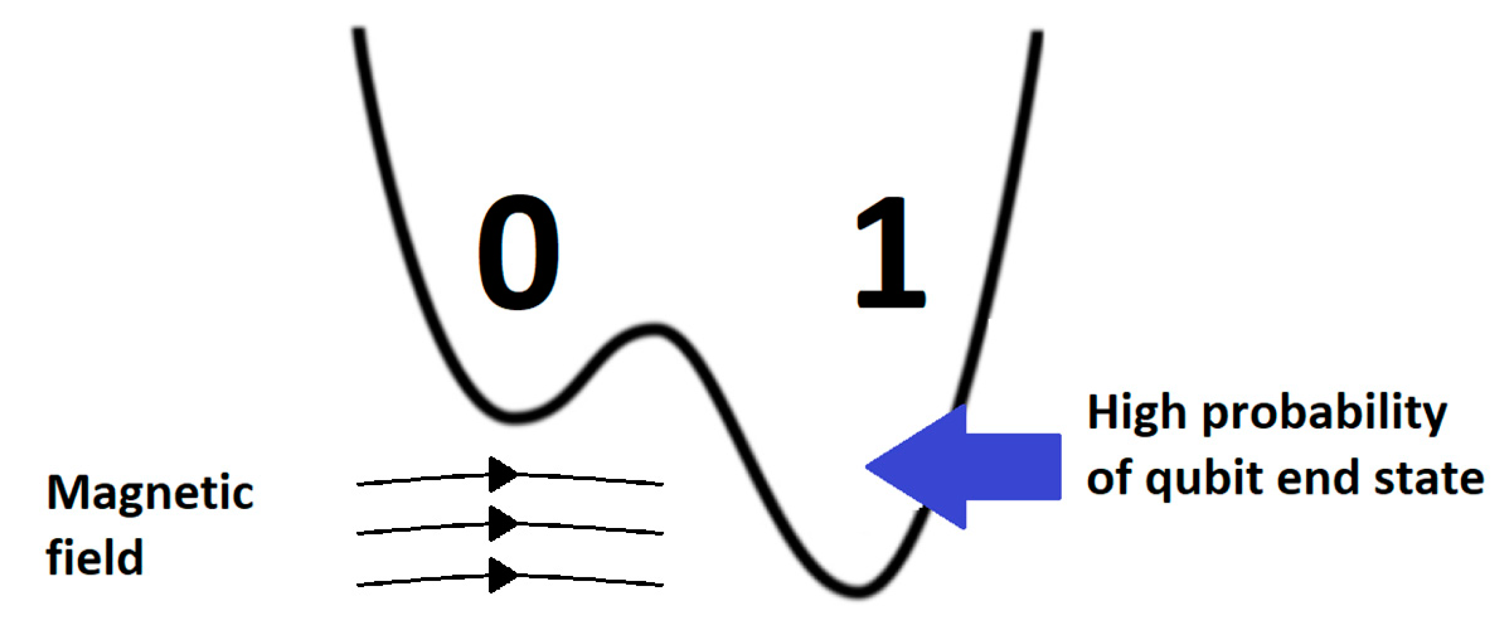
Qubits are the lowest energy states of the superconducting loops in QPU using this technology. These processors do not use quantum versions of logic gates but generate energy diagrams with two valleys known as double-well potential. Each of the valleys corresponds to states 0 and 1 respectively. The qubit collapses to one of these valleys at the end of the process. However, it is possible to control the probability that the qubit collapses to one state or the other. To do this, the qubit is programmed by applying subjecting it to an external magnetic field. The field tilts the energy diagram increasing the probability of a qubit collapsing into a particular valley, as can be seen in
Figure 3 [
33].
This indicates how these processors operate in superposition. In addition, these qubits can be interlocked together with devices called couplers. A coupler can cause two qubits to collapse into the same or opposite states. These two interlocked qubits can be interpreted as a single object with four possible states [
34]. In short, although unlike other quantum technologies quantum annealing technology cannot be used for general purposes, the work of the D-Wave Systems company claims that it represents a very interesting approach to optimization problems [
35].
Table 1 summarizes the current technologies related to quantum computing that have been addressed in this section.
2.7. Quantum Algorithms and Main Applications for Quantum Computing
Quantum algorithms are those that are executed on quantum computers and have computational advantages over algorithms executed on conventional computers.
The quantum paradigm does not consist of doing the same thing more quickly, but in executing quantum algorithms that allow certain operations to be performed in a totally different way, and, on many occasions, far more efficiently.
These advantages are usually in terms of speed and efficiency, especially in those problems that are not tractable on conventional computers. Quantum algorithms could present a substantial advantage when employing techniques that classical computation is unable to achieve, such as superposition or entanglement.
The computational complexity of an algorithm increases as the size of the algorithm increases in terms of variables or inputs. Complexity theory classifies problems into classes according to the relationship between the size of the problem and the resources required (mainly computational time and memory space) to reach a solution [
36].
Problems are classified as (i) easy, those that use a constant number of operations or grow at a log
2(n) logarithmic rate; (ii) tractable, when their operations grow with a polynomial cost; (iii) intractable, when they grow at an exponential rate. If polynomial algorithms are found for problems that are currently classified as intractable, they undergo a change in their classification [
37].
For example, if an algorithm must choose the optimal path among a million options, these paths must be encoded and analyzed in bits or qubits depending on whether it is run on a classical or quantum computer. A classical computer would need to analyze each of these paths one by one, requiring in the order of N/2 steps, i.e., 500,000 operations. However, a quantum computer can find an optimal path by taking advantage of quantum parallelism and finding the solution in sqrt(N) operations, i.e., 1000 tries.
In another class of algorithms, the quantum advantage is even greater. A conventional computer can perform the Fourier transform using n2n logic gates, while a quantum computer can solve a transform in n2, which translates into exponential savings.
Thus, the advantage that quantum computing brings to the resolution of the transform is that for n qubits, the calculations are performed in 2n amplitudes. This makes it possible to efficiently solve many problems that are not solvable on an ordinary computer.
Similarly, one of the possibilities of quantum computing is the application of quantum algorithms to artificial intelligence and machine learning applications [
38]. Through machine learning, these algorithms can automatically learn to recognize recurring patterns from huge amounts of data. In these applications, there are a large number of combinations of analysis and computation, which in computational terms implies a very expensive optimization problem [
39].
One of the main challenges of quantum computing are applications in physics and chemistry. The quantum characteristics of these devices give them the potential to solve molecular electronic structure simulation problems. These simulations have a wide range of applications such as the design of new materials or the discovery of new drugs [
40].
Quantum computing can have a major impact on storage devices, permitting the storage of huge amounts of data in a very small space [
9].
Many industries such as logistics, financial services or telecommunications require optimization algorithms. Quantum computing can be used to solve a wide variety of these problems, as in the application of Monte Carlo methods [
35].
Another application for a quantum system is to increase the variety in
models for pattern identification, recommendation systems, automatic classification and autonomous decision making [
41].
An important role of quantum computing is also expected in the fields of cryptocurrencies and network security mechanisms. The computing power of quantum computers could render current encryption algorithms obsolete and open doors to new ways of protecting information and risk analysis [
42,
43].
3. Quantum Approaches for Machine Learning
In this section, several available approaches for quantum machine learning are presented.
3.1. Variational Quantum Circuits for Machine Learning
The quantum mode operation of the set of qubits is very fragile and unstable. In fact, the instability of the set of operating qubits of a quantum computer increases with the number of qubits and is related to the quality of the materials from which they are made. For this reason, the coherence time in which the qubits are stable is limited.
To efficiently solve problems such as unstructured database searches [
44], the use of thousands of qubits with low error rates and high coherence times will be required. These quantum computers are not yet available, but noisy intermediate-scale quantum (NISQ) computers can already be used [
45]. However, these computers are composed of numerous noisy qubits that remain stable for very few nanoseconds.
Variational quantum algorithms (VQAs) [
46,
47,
48,
49] use classical optimizers to train parameterized quantum circuits and represent an advancement in quantum computing running on NISQ computers [
50].
Variational algorithms can be the basis for numerous applications, for example, in the design of a quantum classifier. The algorithm is similar in operation to a classical support-vector machine.
In machine learning, support-vector machines or SVMs are supervised learning models for solving classification and regression problems. Basically, SVMs build models capable of predicting whether a new point belongs to one category or another. Similarly, the quantum variational circuit performs hyperplane slices like a conventional SVM. On the other hand, kernel functions are used to solve nonlinear classification problems using linear classifiers. Classifiers based on quantum logic have no advantage over classical computers when the kernel function can be computed efficiently on a classical computer.
However, on many occasions, when the feature space is very large and kernel functions are hard to find, quantum computing can be very useful [
38].
The variational algorithm uses the Hilbert space in which the quantum processor operates to find the optimal hyperplane cut in the same way as a classical support-vector machine. The algorithm is run for training and for classification. The training stage uses an already classified dataset.
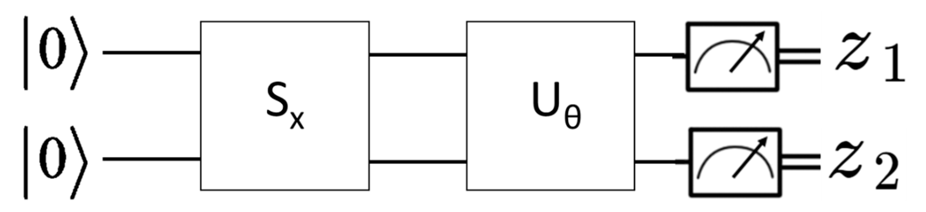
The algorithm is composed of three parts: (i) state preparation or feature map where the input data x are encoded; (ii) model circuit or optimization circuit with input parameters θ; and (iii) measurement stage z as shown in the following equation. A diagram with the three stages is shown in
Figure 4.
3.2. Quantum Convolutional Neural Networks
Convolutional neural networks (CNNs) are a type of neural network in which neurons act as receptive agents, mimicking neurons in the primary visual cortex of a biological brain. The main applications of this type of network are related to visual computer tasks, such as, for example, image classification and segmentation, precision medicine or optical character recognition [
51].
A CNN generally consists of three layers: a convolution layer, a pooling layer and fully connected layer. The convolution layer computes new pixel values from a linear combination of neighboring pixels with specific weights. The pooling layer aims to reduce the size of the feature map. Finally, the fully connected layer obtains the output through a linear combination of the remaining pixels with specific weights. The weights are calculated through training the neural network with an input dataset.
In the quantum version of this neural network, there is an additional first step of the convolution layer, encoding the image data into a quantum state.
The developed model of a quantum convolutional neural network (QCNN) in [
52] performs well against noise in image recognition applications. In addition, the parameters it uses are independent of the size of the inputs, making it a suitable solution for currently available noisy quantum devices.
In study [
53], a QCNN is used for quantum phase recognition (QPR) applications. In the experiment, the model discovers whether a quantum state belongs to a particular quantum phase. In addition, quantum error correction (QEC) optimization is performed, which consists of optimizing error correction in real experimental environments when the error model is unknown.
QCNNs require fewer parameters to obtain similar results compared to conventional convolutional neural networks. Therefore, both quantum and conventional large-scale neural networks can solve complex machine learning problems, but as the growth of Hilbert spaces is exponential, the quantum alternative is more efficient.
3.3. Quantum Distributed or Federated Machine Learning
One of the main limitations of quantum convolutional neural networks (QCNN) is that they are a centralized solution. The generation of deep learning models requires a huge amount of data. Some applications have public datasets for research, but in most advanced processes it is necessary to collect specific data in fields such as medical imaging or natural language processing (NLP). As sharing data from these applications can infringe on user rights, federated learning [
54] can solve the problem if the model is trained directly at the user’s source, and what is shared in the cloud are the parameters of the trained model. The components of a federated machine learning system are the central node and several client nodes that send the parameters calculated in the training to the central node.
Quantum distributed training consists of performing the training of a neural network through several quantum computers (that act as central and client nodes), with the objective of reducing the time needed to train the network. Hybrid quantum-classical neural networks can be used, although the concept is equally applicable to any type of machine learning model.
Some studies on network training [
55,
56] show that similar levels of precision can be obtained more quickly with quantum distributed machine learning. However, for the integration of quantum computers in future communication systems, it is necessary to create large-scale distributed quantum networks that surpass the quantum networks currently emerging [
57].
3.4. Quantum Reinforcement Learning
In addition to supervised and unsupervised learning, there is a third area of machine learning known as reinforcement learning (RL). In reinforcement learning, intelligent agents make decisions to maximize cumulative reward. The scope of this approach is oriented towards exploring the unknown and exploiting available knowledge [
58].
Conventional reinforcement learning systems have three main elements: (i) policy, (ii) reward function, and (iii) model of the environment. However, the implementation of quantum algorithms could be substantially different from traditional ones. Quantum machine learning has a potential acceleration of
O(sqrt(N)) for machine learning algorithms using quantum reinforcement learning [
59].
In Ref. [
60] quantum variational circuits are used to replace neural networks in reinforcement algorithms. Their conclusion is that QVC facilitates reaching a higher efficiency than traditional neural networks.
In Ref. [
61] another experiment is presented in which the agent learning process is accelerated by using a quantum communication channel.
4. Materials and Methods
In this section, a variational quantum circuit is implemented. In addition, an experimental setup is defined for quantum simulation and execution applied to the detection of weak signals of the future.
4.1. Design of a Variational Quantum Algorithm for Quantum Machine Learning
As previously defined, a variational quantum algorithm is composed of a state preparation stage, a model circuit, and a measurement stage. The model circuit acts on a quantum state in which the input data x have been encoded.
The first step is to prepare the circuit by putting the qubits in a superposition state. To do this, Hadamard gates are introduced, which create a basic 50–50 superposition. This means that, when measuring the state, a result of ‘0’ or ‘1’ will be obtained with a 50% probability for each of the states. The Hadamard gate maps the Z-axis to the X-axis (and vice versa).
Once the quantum computer is in a superposition state, entanglement is used for state preparation Sx, which consists of embedding the classical data in a quantum state. The most common way to do this operation is amplitude encoding [
62,
63,
64,
65]. As a result, the coordinates of a vector are mapped into the amplitude values of a quantum state.
With this step, it is possible to map the input data in a nonlinear way into a quantum state, as can be seen in the following equation, which assumes a quantum feature map:
Entanglement is achieved by combining Z quantum gates and two-qubit CNOTs as can be seen in
Figure 5. This circuit acts on the initial state |00〉 and does not need to have a high depth to fulfill its function [
38], and basically consists of Hadamard gates and a diagonal gate in the Pauli Z-basis [
66].
The Z-gate changes the sign of the amplitude when applied to the state of the qubit |1〉 and leaves it unchanged when operating with a qubit in the |0〉 state. Thus, the Z-gate shifts the qubit along the interval on the Bloch sphere over the surface of the sphere from |0〉 to |1〉, rotating values around the z-axis.
The CNOT or controlled NOT gate operates two-qubit registers. The CNOT inverts the second qubit if the first qubit has the state |1〉. However, the CNOT does not vary the state of the second qubit if the first qubit has the state |0〉.
Once the feature map has been created and the input data are encoded in qubit amplitudes, it is necessary to apply a model circuit Uθ, where θ is a set of classical parameters belonging to R2n(l+1). The parameters θ are optimized during the training phase.
The model circuit is composed of one-qubit quantum gates and quantum gates controlled by an additional single qubit. In this way, the algorithm retains a low depth [
41]. The circuit is composed of
l layers, being
l = 5 in the experiment performed. By increasing the depth with larger
l, higher success rates are expected [
38].
The model circuit is shown in
Figure 6. If a qubit with the state α|0〉 + β|1〉 is introduced at the input of a Y gate, the output will have the state β i|0〉 − α i|1〉, so it works as a combination of gates X and Z.
Once the model is executed, for a problem of classification ‘y’ with two labels, a binary measurement is performed on the output state of the qubits.
The probability of obtaining a specific outcome in the classification is described in the next equation:
for a Boolean function f:{0,1}
n.
For decision making, the system is executed R times to obtain an empirical distribution.
An alternative to this circuit is to use a classical SVM to perform the classification instead of using a variational quantum circuit. In this case, the kernel is estimated directly within the quantum computer for a pair of input data [
38].
4.2. Application to the Detection of Weak Signals of the Future
Weak signals are indicators of incipient changes that will have a future impact [
67]. Even for experts, the detection of these events is complicated as their impact is as yet unpredictable.
The available studies on these types of signals are mostly qualitative [
68], valid only for specific applications [
69,
70,
71] and based on the opinion of experts and other stakeholders [
72]. Even in cases where quantitative analysis is used, these studies are based only on structured data [
73].
However, a system has been developed to assist experts in the detection of weak signals that are quantitative, multipurpose, and drawn from various types of unstructured data sources. This system has been successfully applied in various sectors such as solar panels [
74], artificial intelligence [
75] and remote sensing [
44].
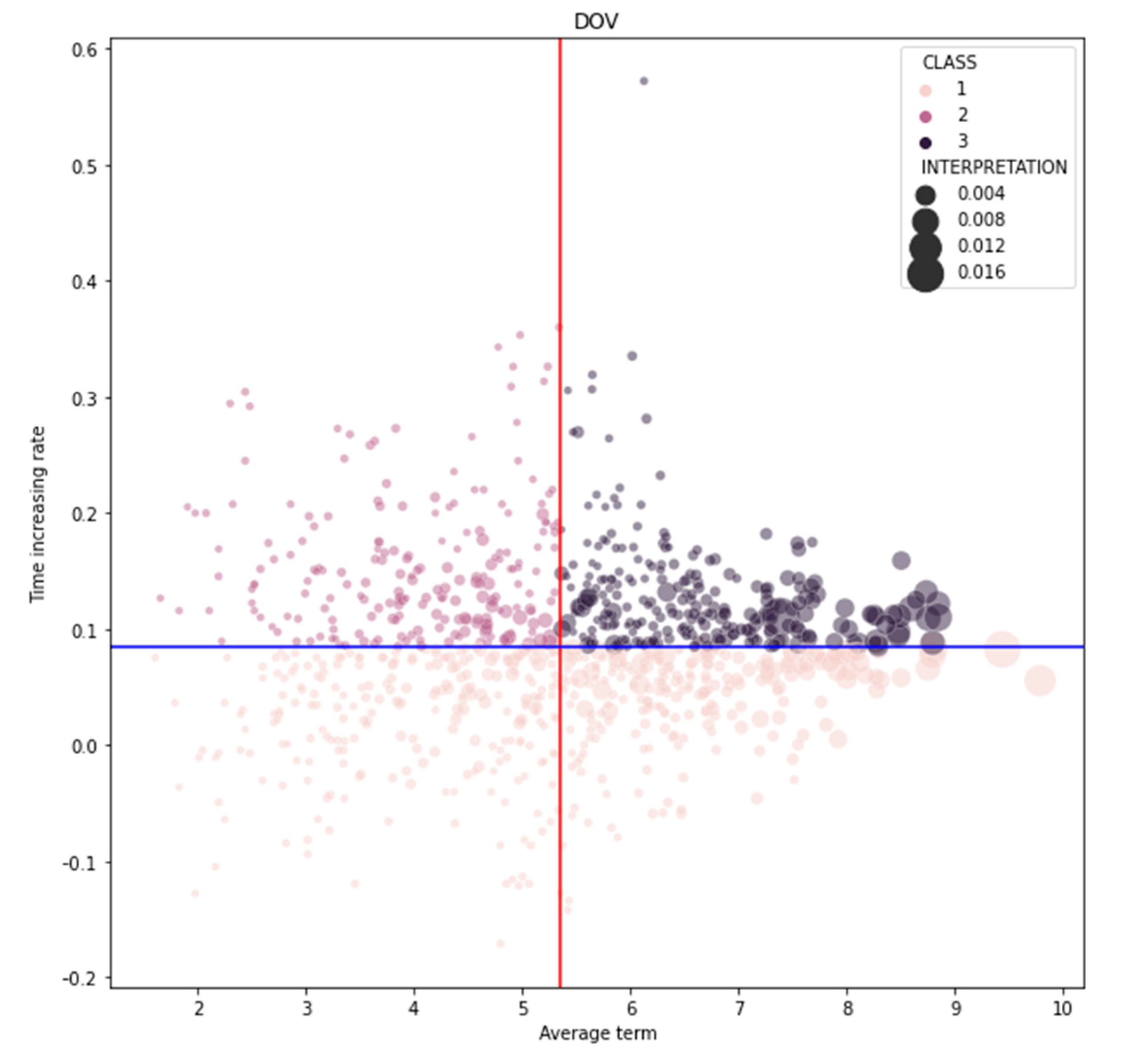
The data used by the system are all kinds of documents from a variety of sources, such as scientific articles, newspaper articles and social media posts. One of the most important phases of the system is text mining, in which all the words in these documents are classified into three different data classes as can be seen in
Figure 7, where data are classified in three different classes: (i) possible weak signals, (ii) strong signals (those signals that have already reached the necessary impact to be known by a wide audience), and (iii) noise (words and expressions in which there has been no increase in usage). The two main factors are the average frequency of each word and a time weighted
increase rate to give more value to the most recent occurrences.
Two different keyword maps are created with this structure. The first one is based on the ‘degree of diffusion’ or
DoD, and the second one is based on the ‘degree of visibility’ or
DoV. These two dimensions are part of the model of a weak signal by Hiltunen [
76].
The degree of diffusion (DoD) uses the total number of documents where the keyword appears as an average frequency to define an increasing rate considering different periods of time. The degree of visibility (DoV) uses the total number of appearances of each keyword (independently of the number of documents) as an average frequency, to define an increasing rate considering again different periods of time. The keyword is considered a weak signal when in both keyword maps for DoD and DoV it is classified as weak signal.
In available studies, the opinion of experts [
44] is used to define the thresholds that divide the word cloud into these three clusters. However, current results show that many of the expressions detected as weak signals may be false positives.
For this reason, a machine learning system to define the clusters in an automatic way may be more appropriate.
The process consists of creating a training set considering only those words classified as weak signals in both DoV and DoD maps. Then, the classifier is applied to classify the rest of the words to reduce the number of false positives detected.
In addition, the applications in which the system has been used has had an input dataset of about 90 k documents, which implies about 150 million words. The processing advantage offered by quantum computers is a very interesting advance in the classification of these words.
In the next section, the system is analyzed by applying the quantum classifier described in this section to the medical imaging sector.
4.3. Quantum Circuit Simulation and Execution Framework
Qiskit [
77] is a quantum simulation tool created by IBM for quantum software development using the Python programming language. Its functionalities are divided into four different components: (i) Terra, which provides tools for programming quantum circuits with levels close to machine code; (ii) Aqua, which provides already programmed quantum algorithms for the realization of applications in the fields of chemistry, AI, optimization and finance; (iii) Aer,
(a) software simulator on small quantum devices; (iv) Ignis, a tool that characterizes noise in quantum devices to mitigate errors.
On the other hand, in IBM Quantum Experience [
78] it is possible to access IBM quantum computers remotely to implement and run quantum algorithms in real environments. IBM’s quantum processors are fabricated using superconducting transmon qubits that are at temperatures near absolute zero at IBM’s New York research center.
For example, a test can be performed by testing a basic circuit as shown in
Figure 8, consisting of a Hadamard gate applied only to one of the qubits and a CNOT gate controlled by this same qubit.
If the simulation of the circuit is performed using the Aer component of Qiskit, the result seen in
Figure 9a is obtained, in which there is approximately a 50% probability of obtaining the state |00〉 and another 50% of obtaining |11〉. However, when the same circuit is run on the 5-bit quantum computer ‘ibmq_santiago’ through IBM Quantum Experience, the result shown in
Figure 9b is obtained, in which after running the circuit
for 1024 shots, the states |01〉 and |10〉 are also found. This occurs because the simulator represents a perfect quantum device, but the real quantum device is noisy and susceptible to errors.
There are other frameworks for quantum programming such as Penny Lane [
79], developed by Xanadu under the Apache 2.0 License. In addition, it allows interaction with real hardware through Amazon Braket [
80] which allows access to several real quantum computers of various technologies.
5. Results
To perform the experiment, more than 40,000 ScienceDirect scientific articles, more than 1500 New York Times newspaper articles and more than 50,000 Twitter tweets between 2007 and 2017 were extracted and divided into 11 groups of documents from every year for the analysis. All these documents were related to the sector of medical imaging.
A dataset of 937 elements has been generated to detect keywords related to weak signals of the future.
Figure 10 shows the classification of these keywords by defining two thresholds to divide the word cloud as in [
44] according to the
DoV criteria. As previously stated, this simple methodology has the problem that many of the expressions detected as weak signals are false positives.
Table 2 shows some of the output results of the application of the system described in [
44]. The full data set is available.
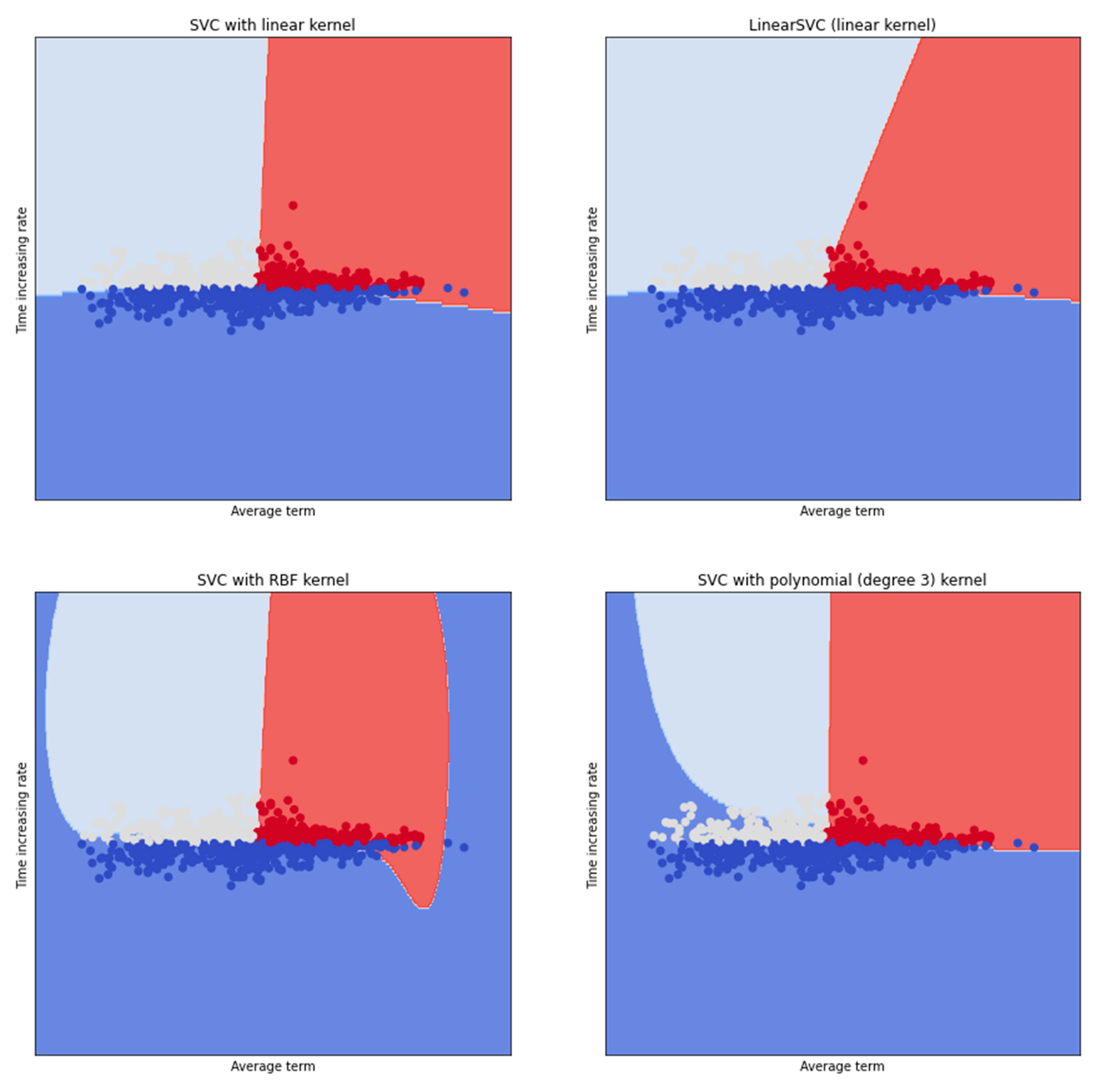
Figure 11 shows the result of applying support vector machines with different kernels in a conventional computer, including linear kernel, linear SVC, radial basis function (RBF) kernel and a polynomial kernel of degree 3.
To encode the data, the function “ZZFeatureMap” of qiskit was used, which encodes and implements the circuit shown in
Figure 5. As a result, the input data was encoded in the amplitudes of a quantum state.
In the first quantum computation test, the complete dataset of 937 elements was used, divided in a training set of 749 elements and a test set of 188 elements. A total of 1024 shots were programmed for each quantum measurement to obtain an accurate probabilistic distribution. However, when using the qiskit simulator and executing the quantum computer ‘ibmq_santiago’, the test did not obtain results after several days of uninterrupted execution. Because of this, it was decided to reduce the initial sample for a second test.
In the second test, a sample of 47 items was used. The training set was composed of 23 items classified as “noise”, 12 items classified as “weak signals” and 12 items classified as “strong signals”. When the system was used for a test set of 8 items classified as “noise”, 3 items classified as “weak signals” and 1 item classified as “strong signals”, a 70.21% success rate was obtained after its execution in ‘ibmq_santiago’. A success rate of 78.72% was obtained after its execution using qiskit quantum simulator. Finally, a success rate of 61.70% was obtained after its execution using the classical algorithm. The algorithm ‘SklearnSVM’ is used to find the performance from classical computing.
These results are shown in
Figure 12 where class A is ‘noise’, class B is ‘weak signals’ and class C is ‘strong signals’.
Another test was performed using a sample of 47 items but only two classes were considered: “weak signals” and “no weak signals”. The latter includes both noise and strong signals. The training set was composed of 33 items classified as “no weak signals” and 14 items classified as “weak signals”. When the system was used for a test set of 11 items classified as “noise” and 1 item classified as “weak signals”, a 70.21% success rate was obtained after its execution in ‘ibmq_santiago’. A success rate of 74.47% was obtained after its execution using qiskit quantum simulator. Finally, a success rate of 80.85% was obtained after its execution using the classical algorithm.
These results are shown in
Figure 13 where class A is ‘no weak signal’ and class B is ‘weak signals’.
The performance results of these tests are shown in
Table 3.
6. Discussion and Conclusions
There is a growing interest in the application of quantum computing to machine learning. For this reason, several quantum algorithms are emerging with the potential to be implemented on current quantum devices. However, because these devices are very noisy, these algorithms must be fast and robust against decoherence.
In addition, there are strong arguments showing that circuits of great simplicity are difficult to simulate on conventional computers [
81,
82]. Some studies such as [
62] claim that there is an exponential improvement in this class of algorithms when the input data are in superposition. However, initially the data are encoded in classical logic and the operations required to encode the data in quantum logic considerably reduce this acceleration. [
38].
In the experiment presented in the previous section, it has been proven that similar success rates can be obtained between classical and quantum computing.
In the first test, a comparative study has been performed for the detection of three different classes. Thus, a distinction has been made between ‘weak signals’, ‘strong signals’ and those expressions that have not led to an increase in their use, i.e., ‘noise’. The results show that the quantum simulator obtained the highest level of success in its prediction, with 78.72%, being much higher than the performance of the classical computer. The quantum computer execution ‘ibmq_santiago’ has resulted in a lower prediction success but also higher than that obtained in the classical computer.
In the second test, the same comparative study was carried out, but considering only two classes. The ‘weak signals’ quadrant has been distinguished from the rest of the points that are classified as ‘no weak signals’ including both ‘noise’ and ‘strong signals’. The results show that the classical computer obtained the highest success rate while the quantum simulator obtained a slightly lower performance. However, the use of the real IBM quantum computer ‘ibmq_santiago’, obtained a success rate of 70.21%, being lower than that obtained using the quantum simulator due to the noise resulting from the available quantum devices.
These results show an influence of the dataset on the performances, to which obtaining a suitable feature map is key. In addition, as stated in [
38], available quantum classifiers do not offer a considerable advantage when the feature vector kernel can be efficiently obtained on a classical computer. In fact, this same source reveals that it is possible to achieve 100% performance if the optimal feature map is available. In future research, it is necessary to further study the potential for improvement if suitable feature maps are detected for other real datasets.
Although quantum computing seems to bring many advantages to machine learning algorithms, the results of this study show that with large datasets both the simulator and the real quantum computer have been unable to present results in less time than a classical computer. The need to encode the data in a quantum state and the need to run each circuit a large number of shots as a measure of robustness to noise confirm that current quantum technology cannot yet be considered an alternative to classical computing [
59].
The four main problems that need to be solved are:
First, encoding the input data is especially complex when compared to data processing, and this complexity may come at a high cost to quantum algorithms, which may lose some of their fast-processing advantage.
Second, the output measurements are not easily interpretable, since qubit entanglement computes many solutions until the states collapse into a particular final state.
Third, quantum computation is thought to offer an advantage to solve large problems, but due to hardware limitations, this has not yet been demonstrated.
Finally, better algorithm evaluation systems are needed to appreciate the advantages of quantum algorithms over classical algorithms.
Some possible sources of improvement have been presented in
Section 3. Quantum convolutional neural networks are giving good results to complex problems and have been shown to be more robust to noise than other quantum alternatives [
52]. Quantum simulator success rates or similar are expected to be attained by the reduction of noise.
On the other hand, the integration of quantum variational circuits in reinforcement learning techniques allows higher efficiencies to be achieved [
60].
Another problem that has been detected is that all these applications are centralized. Although there are some distributed solutions available, they usually combine mixed classical and quantum technologies. Although single quantum devices allow a high level of parallelism, federated machine learning improves the security and privacy of users by not sharing their information in the cloud. However, quantum computers are not yet available to the general public. In the future, distributed solutions may increase the speed of handling complex problems that require large amounts of data to be processed.
This paper has described the technologies available for the implementation of quantum devices. Some of these technologies require extreme conditions for their operation, such as temperatures close to absolute zero. In addition, all these technologies are still under development, so current quantum devices are very noisy and have different fabrication yields. However, several organizations are investing considerable resources in obtaining technologies that demonstrate the supremacy of quantum computing.
In addition, the latest advances related to the field of quantum machine learning have been presented in
Section 3. Next, a possible application for quantum machine learning related to future weak signal detection is presented. In this application, a large number of words and documents are taken into account in the process of detecting future trends. The computational advantage that quantum computing possesses adds immense value to this field.
The experiments performed show promising results on technologies that are still under development. Some of the results show higher efficiencies using quantum computers compared to classical ones. In the future, new methods for the detection of suitable future maps, the combination with other technologies and machine learning algorithms, and the application of distributed solutions will allow major improvements in quantum machine learning applications.
Author Contributions
Conceptualization, I.G.-B., S.M., A.C., Y.M. and J.M.; methodology, I.G.-B., S.M. and J.M.; software, I.G.-B. and S.M.; validation, I.G.-B., S.M., A.C., Y.M. and J.M.; formal analysis, I.G.-B.; investigation, I.G.-B., S.M. and J.M.; resources, I.G.-B., S.M. and Y.M.; data curation, I.G.-B. and S.M.; writing—original draft preparation, I.G.-B., writing—review and editing, I.G.-B., A.C., Y.M. and J.M.; visualization, I.G.-B.; supervision, J.M.; project administration, I.G.-B. and J.M.; funding acquisition, I.G.-B. and J.M. All authors have read and agreed to the published version of the manuscript.
Funding
This research received no external funding.
Institutional Review Board Statement
Not applicable.
Informed Consent Statement
Not applicable.
Acknowledgments
The authors acknowledge Ismael Faro who is Chief Architect of Quantum Computing Cloud and Software at IBM for his help in this work. This research is also part of a PhD from the Department of Electronics Engineering of the Universitat Politècnica de València.
Conflicts of Interest
The authors declare no conflict of interest.
References
- Moore, G.E. Cramming more components into integrated circuits, Reprinted from Electronics, volume 38, number 8, April 19, 1965, pp.114 ff. IEEE Solid State Circuits Soc. Newsl. 2006, 11, 33–35. [Google Scholar] [CrossRef]
- Martín-Palma, R.J. Quantum tunneling in low-dimensional semiconductors mediated by virtual photons. AIP Adv. 2020, 10, 015145. [Google Scholar] [CrossRef]
- Benioff, P. Quantum mechanical models of Turing machines that dissipate no energy. Phys. Rev. Lett. 1982, 48, 1581–1585. [Google Scholar] [CrossRef]
- Turing, A.M. On Computable Numbers, with an Application to the Entscheidungsproblem. Proc. Lond. Math. Soc. 1937, 42, 230–265. [Google Scholar] [CrossRef]
- Trabesinger, A. Quantum simulation. Nat. Phys. 2012, 8. [Google Scholar] [CrossRef]
- Nielsen, M.A.; Chuang, I.L. Quantum Computation and Quantum Information; Cambridge University Press: Cambridge, MA, USA, 2010. [Google Scholar]
- Bloch, F. Nuclear induction. Phys. Rev. 1946, 70, 460–474. [Google Scholar] [CrossRef]
- Yorke, B.A.; Beddard, G.; Owen, R.L.; Pearson, A.R. Time-resolved crystallography using the Hadamard transform. Nat. Methods 2014, 11, 1131–1134. [Google Scholar] [CrossRef] [PubMed]
- Ruiz, I.E.K. Quatum Computing: Practical applications that classical computing cannot solve. Bachelor’s Thesis, University Carlos III, Madrid, Spain, 2019. [Google Scholar]
- Yamaguchi, K.; Watamura, N.; Hotta, M. Quantum information capsule and information delocalization by entanglement in multiple-qubit systems. Phys. Lett. A 2019, 383, 1255–1259. [Google Scholar] [CrossRef]
- Gibney, E. Hello quantum world! Google publishes landmark quantum supremacy claim. Nature 2019, 574, 461–462. [Google Scholar] [CrossRef]
- Koch, J.; Yu, T.M.; Gambetta, J.; Houck, A.A.; Schuster, D.I.; Majer, J.; Blais, A.; Devoret, M.H.; Girvin, S.M.; Schoelkopf, R.J. Charge-insensitive qubit design derived from the Cooper pair box. Phys. Rev. A 2007, 76, 042319. [Google Scholar] [CrossRef]
- Lucas, A. Using formulations of many np problems. Front. Phys. 2014, 2. [Google Scholar] [CrossRef]
- Wallraff, A.; Schuster, D.I.; Blais, A.; Frunzio, L.; Huang, R.S.; Majer, J.; Schoelkopf, R.J. Strong coupling of a single photon to a superconducting qubit using circuit quantum electrodynamics. Nature 2004, 431, 162–167. [Google Scholar] [CrossRef]
- Cirac, J.I.; Zoller, P. A scalable quantum computer with ions in an array of microtraps. Nature 2000, 404, 579–581. [Google Scholar] [CrossRef]
- Seif, A.; Landsman, K.A.; Linke, N.M.; Figgatt, C.; Monroe, C.; Hafezi, M. Machine learning assisted readout of trapped ion qubits. J. Phys. B At. Mol. Opt. Phys. 2018, 51. [Google Scholar] [CrossRef]
- Eschner, J. Quantum Computation with Trapped Ions; Institut de Ciències Fotòniques: Castelldefels, Spain, 2006. [Google Scholar]
- Monroe, C.R.; Schoelkopf, R.J.; Lukin, M.D. Quantum connections. Sci. Am. 2016, 314, 50–57. [Google Scholar] [CrossRef] [PubMed]
- Mourik, V.; Zuo, K.; Frolov, S.M.; Plissard, S.R.; Bakkers, E.; Kouwenhoven, L.P. Signatures of Majorana fermions in hybrid superconductor-semiconductor nanowire devices. Science 2012, 336, 1003–1007. [Google Scholar] [CrossRef]
- Zhang, H.; Liu, C.X.; Gazibegovic, S.; Xu, D.; Logan, J.A.; Wang, G.; van Loo, N.; Boomer, J.D.S.; de Moor, M.W.A.; Car, D.; et al. RETRACTED ARTICLE: Quantized Majorana conductance. Nature 2018, 556, 74–79. [Google Scholar] [CrossRef]
- Frolov, S. Quantum computing’s reproducibility crisis: Majorama fermions. Nature 2021, 592, 350–352. [Google Scholar] [CrossRef]
- Vandersypen, L.M.K.; Eriksson, M.A. Quantum computing with semiconductor spins. Phys. Today 2019, 72, 38. [Google Scholar] [CrossRef]
- Loss, D.; DiVincenzo, D.P. Quantum computation with quantum dots. Phys. Rev. A Am. Phys. Soc. 1998, 57, 120–126. [Google Scholar] [CrossRef]
- Ekimov, A.I.; Efros, A.L.; Onushchenko, A.A. Quantum size effect in semiconductor microcrystals. Solid State Commun. 1985, 56, 921–924. [Google Scholar] [CrossRef]
- Bluhm, H.; Foletti, S.; Neder, I.; Rudner, M.; Mahalu, D.; Umansky, V.; Yacoby, A. Dephasing time of GaAs electron-spin qubits coupled to a nuclear bath exceeding 200 μs. Nat. Phys. 2010, 7, 109–113. [Google Scholar] [CrossRef]
- Wang, S.; Querner, C.; Dadosh, T.; Crouch, C.H.; Novikov, D.S.; Drndic, M. Collective fluorescence enhancement in nanoparticle clusters. Nat. Commun. 2011, 2. [Google Scholar] [CrossRef][Green Version]
- Watzinger, H.; Kukučka, J.; Vukušić, L.; Gao, F.; Wang, T.; Schäffler, F.; Zhang, J.J.; Katsaros, G. A germanium hole spin qubit. Nat. Commun. 2018, 9, 3902. [Google Scholar] [CrossRef] [PubMed]
- Trauzettel, B.; Bulaev, D.V.; Loss, D.; Burkard, G. Spin qubits in graphene quantum dots. Nat. Phys. 2007, 3, 192–196. [Google Scholar] [CrossRef]
- Guerreschi, G.G.; Park, J. Two-step approach to scheduling quantum circuits. Quantum Sci. Technol. 2018, 3, 0345003. [Google Scholar] [CrossRef]
- Brotons-Gisbert, M.; Proux, R.; Picard, R.; Andres-Penares, D.; Branny, A.; Molina-Sánchez, A.; Sánchez-Royo, J.F.; Gerardot, B.D. Out-of-plane orientation of luminescent excitons in two-dimensional indium selenide. Nat. Commun. 2019, 10, 3913. [Google Scholar] [CrossRef]
- Wang, J.; Paesani, S.; Ding, Y.; Santagati, R.; Skrzypczyk, P.; Salavrakos, A.; Tura, J.; Augusiak, R.; Mancinska, L.; Bacco, D.; et al. Multidimensional quantum entanglement with large-scale integrated optics. Science 2018, 360, 285–291. [Google Scholar] [CrossRef]
- Arrazola, J.M.; Bergholm, V.; Brádler, K.; Bromley, T.R.; Collins, M.J.; Dhand, I.; Fumagalli, A.; Gerrits, T.; Goussey, A.; Helt, L.G.; et al. Quantum circuits with many photons on a programmable nanophotonic chip. Nature 2021, 591, 54–60. [Google Scholar] [CrossRef]
- Bian, Z.; Chudak, F.; Israel, R.B.; Lackey, B.; Macready, W.G.; Roy, A. Mapping constrained optimization problems to quantum annealing with application to fault diagnosis. Front. ICT 2016, 3, 14. [Google Scholar] [CrossRef]
- Johnson, M.W.; Amin, M.H.S.; Gildert, S.; Lanting, T.; Hamze, F.; Dickson, N.; Harris, R.; Berkley, A.J.; Johansson, J.; Bunyk, P.; et al. Quantum annealing with manufactured spins. Nature 2011, 473, 194–198. [Google Scholar] [CrossRef]
- King, A.D.; Raymond, J.; Lanting, T.; Isakov, S.V.; Mohseni, M.; Poulin-Lamarre, G.; Ejtemaee, S.; Bernoudy, W.; Ozfidan, I.; Smirnov, A.Y.; et al. Scaling advantage over path-integral Monte Carlo in quantum simulation of geometrically frustrated magnets. Nat. Commun. 2021, 12. [Google Scholar] [CrossRef] [PubMed]
- Cobham, A. The intrinsic computational difficulty of functions. In Logic, Methodology and Philosophy of Science, Proceedings of the 1964 International Congress, Jerusalem, Israel, 26 August–2 September 1964; North-Holland Publishing Company: Amsterdam, The Netherlands, 1965; pp. 24–30. [Google Scholar]
- Goldreich, O. Computational Complexity: A Conceptual Perspective; Cambridge University Press: Cambridge, MA, USA, 2008. [Google Scholar]
- Havlíček, V.; Córcoles, A.D.; Temme, K.; Harrow, A.W.; Kandala, A.; Chow, J.M.; Gambetta, J.M. Supervised learning with quantum-enhanced feature spaces. Nature 2019, 567, 209–212. [Google Scholar] [CrossRef] [PubMed]
- Barkoutsos, P.K.I.; Nannicini, G.; Robert, A.; Tavernilli, I.; Woerner, S. Improving variational quantum optimization using CVaR. Quantum 2020, 4, 256. [Google Scholar] [CrossRef]
- Liu, H.; Hao Low, G.; Steiger, D.S.; Häner, T.; Reiher, M.; Troyer, M. Prospects of Quantum Computing for Molecular Sciences. arXiv 2021, arXiv:2102.10081. [Google Scholar]
- Schuld, M.; Bocharov, A.; Svore, K.; Wiebe, N. Circuit-centric quantum classifiers. Phys. Rev. A 2020, 101, 032308. [Google Scholar] [CrossRef]
- Woerner, S.; Egger, D.J. Quantum risk analysis. Nat. Quantum Inf. 2019, 5, 15. [Google Scholar] [CrossRef]
- Eskandarpour, R.; Gokhale, P.; Khodaei, A.; Chong, F.T.; Passo, A.; Bahramirad, S. Quantum Computing for Enhancing Grid Security. IEEE Trans. Power Syst. 2020, 35, 4135–4137. [Google Scholar] [CrossRef]
- Griol-Barres, I.; Milla, S.; Cebrián, A.; Fan, H.; Millet, J. Detecting weak signals of the future: A system implementation based on Text Mining and Natural Language Processing. Sustainability 2020, 12, 7848. [Google Scholar] [CrossRef]
- Preskill, J. Quantum computing in the NISQ era and beyond. Quantum 2018, 2, 79. [Google Scholar] [CrossRef]
- Zhou, L.; Wang, S.-T.; Choi, S.; Pichler, H.; Lukin, M.D. Quantum Approximate Optimization Algorithm: Performance, Mechanism, and Implementation on Near-Term Devices algorithm. arXiv 2019, arXiv:1812.01041v2. [Google Scholar]
- Farhi, E.; Goldstone, J.; Gutmann, S. A quantum approximate optimization algorithm. arXiv 2014, arXiv:1411.4028. [Google Scholar]
- McClean, J.R.; Romero, J.; Babbush, R.; Aspuru-Guzik, A. The theory of variational hybrid quantum-classical algorithms. New J. Phys. 2016, 18, 023023. [Google Scholar] [CrossRef]
- Romero, J.; Olson, J.P.; AspuruGuzik, A. Quantum autoencoders for efficient compression of quantum data. Quantum Sci. Technol. 2017, 2, 045001. [Google Scholar] [CrossRef]
- Cerezo, M.; Arrasmith, A.; Babbush, R.; Benjamin, S.C.; Endo, S.; Fujii, K.; McClean, J.R.; Mitarai, K.; Yuan, X.; Cincio, L.; et al. Variational Quantum Algorithms. arXiv 2020, arXiv:2012.09265. [Google Scholar]
- Le Cun, Y.; Bengio, Y.; Hinton, G. Deep learning. Nature 2015, 521, 436–444. [Google Scholar] [CrossRef] [PubMed]
- Wei, S.; Chen, Y.; Zhou, Z.; Long, G. A Quantum Convolutional Neural Network on NISQ Devices. arXiv 2021, arXiv:2104.06918. [Google Scholar]
- Cong, I.; Choi, S.; Lukin, M.D. Quantum convolutional neural networks. Nat. Phys. 2019, 15, 1273–1278. [Google Scholar] [CrossRef]
- McMahan, B.; Moore, E.; Ramage, D.; Hampson, S.; Arcas, B.A. Communication-efficient learning of deep networks from decentralized data. In Proceedings of the 20th International Conference on Artificial Intelligence and Statistics, Ft. Lauderdale, FL, USA, 20–22 April 2017; pp. 1273–1282. [Google Scholar]
- Yen-Chi Chen, S.; Yoo, S. Computational Science Initiative. arXiv 2021, arXiv:2103.12010. [Google Scholar]
- Chehimi, M.; Saad, W. Quantum Federated Learning with Quantum Data. arXiv 2021, arXiv:2106.00005. [Google Scholar]
- Pirandola, S.; Braunstein, S.L. Physics: Unite to build a quantum internet. Nature 2016, 532, 169–171. [Google Scholar] [CrossRef] [PubMed]
- Sutton, R.; Barto, A.G. Reinforcement Learning: An Introduction; MIT Press: Cambridge, MA, USA, 1998. [Google Scholar]
- Biamonte, J.; Wittek, P.; Pancotti, N.; Rebentrost, P.; Wiebe, N.; Lloyd, S. Quantum machine learning. Nature 2017, 549, 195–202. [Google Scholar] [CrossRef] [PubMed]
- Lockwood, O.; Si, M. Reinforcement learning with quantum variational circuits. In Proceedings of the 16th AAAI Conference on Artificial Intelligence and Interactive Digital Entertainment (AIIDE-20), Palo Alto, CA, USA, 19–23 October 2020. [Google Scholar]
- Saggio, V.; Asenbeck, B.E.; Hamann, A.; Strömberg, T.; Schiansky, P.; Dunjko, V.; Friis, N.; Harris, N.C.; Hockberg, M.; Englund, D.; et al. Experimental quantum speed-up in reinforcement learning agents. Nature 2021, 591, 229–233. [Google Scholar] [CrossRef]
- Rebentrost, P.; Mohseni, M.; Lloyd, S. Quantum support vector machine for big data classification. Phys. Rev. Lett. 2014, 113, 130503. [Google Scholar] [CrossRef] [PubMed]
- Kerenedis, I.; Prakash, A. Quantum recommendation systems. arXiv 2016, arXiv:1603.08675. [Google Scholar]
- Wiebe, N.; Braun, D.; Lloyd, S. Quantum algorithm for data fitting. Phys. Rev. Lett. 2012, 109, 050505. [Google Scholar] [CrossRef]
- Schuld, M.; Fingerhuth, M.; Petruccione, F. Implementing a distance-based classifier with a quantum interference circuit. EPL 2017, 119, 60002. [Google Scholar] [CrossRef]
- Mitarai, K.; Negoro, M.; Kitagawa, M.; Fujii, K. Quantum circuit learning. arXiv 2018, arXiv:1803.00745. [Google Scholar] [CrossRef]
- Ansoff, H.I. Managing Strategic Surprise by Response to Weak Signals. Calif. Manag. Rev. 1975, 18, 21–33. [Google Scholar] [CrossRef]
- McGrath, J.; Fischetti, J. What if compulsory schooling was a 21st century invention? Weak signals from a systematic review of the literature. Int. J. Educ. Res. 2019, 95, 212–226. [Google Scholar] [CrossRef]
- Koivisto, R.; Kulmala, I.; Gotcheva, N. Weak signals and damage scenarios—Systematics to identify weak signals and their sources related to mass transport attacks. Technol. Forecast. Soc. Chang. 2016, 104, 180–190. [Google Scholar] [CrossRef]
- Davis, J.; Groves, C. City/future in the making: Masterplanning London’s Olympic legacy as anticipatory assemblage. Futures 2019, 109, 13–23. [Google Scholar] [CrossRef]
- Awan, F.M.; Saleem, Y.; Minerva, R.; Crespi, N. A Comparative Analysis of Machine/Deep Learning Models for Parking Space Availability Prediction. Sensors 2020, 20, 322. [Google Scholar] [CrossRef]
- Van Veen, B.L.; Ortt, R.; Badke-Schaub, P. Compensating for perceptual filters in weak signal assessments. Futures 2019, 108, 1–11. [Google Scholar] [CrossRef]
- Thorleuchter, D.; Van den Poel, D. Idea mining for webbased weak signal detection. Futures 2015, 66, 25–34. [Google Scholar] [CrossRef]
- Griol-Barres, I.; Milla, S.; Millet, J. Implementación de un sistema de detección de señales débiles de futuro mediante técnicas de minería de textos. (Implementation of a weak signal detection system by text mining techniques). Rev. EsDoc. Cient. 2019, 42, 234. [Google Scholar] [CrossRef]
- Griol, I.; Milla, S.; Millet, J. Improving strategic decision making by the detection of weak signals in heterogeneous documents by text mining techniques. AI Commun. 2019, 32, 347–360. [Google Scholar] [CrossRef]
- Hiltunen, E. The future sign and its three dimensions. Futures 2007, 40, 247–260. [Google Scholar] [CrossRef]
- Qiskit. Available online: https://qiskit.org/ (accessed on 30 May 2021).
- IBM Quantum Experience. Available online: https://quantum-computing.ibm.com/ (accessed on 30 May 2021).
- Penny Lane. Available online: https://pennylane.ai/ (accessed on 30 May 2021).
- Amazon Bracket. Available online: https://aws.amazon.com/braket/ (accessed on 30 May 2021).
- Terhal, B.M.; DiVincenzo, D.P. Adaptive quantum computation, constant depth quantum circuits and arthur-merlin games. Quantum Inf. Comput. 2004, 4, 134–145. [Google Scholar]
- Bremner, M.J.; Montanaro, A.; Shepherd, D.J. Achieving quantum supremacy with sparse and noisy commuting quantum computations. Quantum 2017, 1, 8. [Google Scholar] [CrossRef]
Figure 1.
The Block sphere representing a qubit in the state of: (a) |0〉 and (b) after applying a Hadamard gate to (a).
Figure 1.
The Block sphere representing a qubit in the state of: (a) |0〉 and (b) after applying a Hadamard gate to (a).
Figure 2.
Superconducting qubits with (a) diagram of a transmon, and (b) implementation of a quantum processor unit with 4 transmon qubits.
Figure 2.
Superconducting qubits with (a) diagram of a transmon, and (b) implementation of a quantum processor unit with 4 transmon qubits.
Figure 3.
Quantum annealing allows the application of external magnetic fields to modify the probabilities of a qubit ending state.
Figure 3.
Quantum annealing allows the application of external magnetic fields to modify the probabilities of a qubit ending state.
Figure 4.
Variational quantum algorithm that applies the function f(x, θ) = z, with a state preparation circuit SX, where an input x is encoded, a model circuit Uθ where the parameters θ are applied, and the measurement stage.
Figure 4.
Variational quantum algorithm that applies the function f(x, θ) = z, with a state preparation circuit SX, where an input x is encoded, a model circuit Uθ where the parameters θ are applied, and the measurement stage.
Figure 5.
State preparation circuit SX that maps the training and input data to a quantum feature map.
Figure 5.
State preparation circuit SX that maps the training and input data to a quantum feature map.
Figure 6.
Model circuit Uθ that maps used for the classifier.
Figure 6.
Model circuit Uθ that maps used for the classifier.
Figure 7.
Keyword map showing the three different classes for an application for the detection of weak signals of the future.
Figure 7.
Keyword map showing the three different classes for an application for the detection of weak signals of the future.
Figure 8.
Basic circuit with a Hadamard gate, CNOT gate and binary measurements.
Figure 8.
Basic circuit with a Hadamard gate, CNOT gate and binary measurements.
Figure 9.
Measurements obtained from the execution of the circuit from
Figure 8 by (
a) using the Aer component simulator of Qiskit, and (
b) implementing and executing the circuit in a real quantum computer ‘ibmq_santiago’.
Figure 9.
Measurements obtained from the execution of the circuit from
Figure 8 by (
a) using the Aer component simulator of Qiskit, and (
b) implementing and executing the circuit in a real quantum computer ‘ibmq_santiago’.
Figure 10.
Definition of the three classes (1) weak signals, (2) strong signals and (3) noise, without using machine learning.
Figure 10.
Definition of the three classes (1) weak signals, (2) strong signals and (3) noise, without using machine learning.
Figure 11.
Result of applying support vector machines with different kernels.
Figure 11.
Result of applying support vector machines with different kernels.
Figure 12.
Result of applying quantum SVM algorithm to the input data for three classes where prediction1 is classical computer, prediction2 is quantum simulation and prediction3 is quantum real computer.
Figure 12.
Result of applying quantum SVM algorithm to the input data for three classes where prediction1 is classical computer, prediction2 is quantum simulation and prediction3 is quantum real computer.
Figure 13.
Result of applying quantum SVM algorithm to the input data for two classes where prediction1 is classical computer, prediction2 is quantum simulation and prediction3 is quantum real computer.
Figure 13.
Result of applying quantum SVM algorithm to the input data for two classes where prediction1 is classical computer, prediction2 is quantum simulation and prediction3 is quantum real computer.
Table 1.
Available technologies for quantum computing.
Table 1.
Available technologies for quantum computing.
| Technology | Superconducting Circuits | Ion Traps | Majorana Quasiparticles | Spin Qubits | Photonic Quantum | Quantum Annealing |
|---|
| Description | Superconducting electrodes interconnected by Josephson junctions | Electromagnetic and optical fields to trap and control ions. | Majorana particles and their identical antiparticles act as qubits. | Control spin of electrons in semiconductors. | Optical devices to control photons. | Magnetic fields to alter energy diagrams. |
| Pros | Fast working. Build on the existing semiconductor industry. | Very stable. Highest achieved gate fidelities. | Very stable. Less sensitivity to noise. | Stable. Build on the existing semiconductor industry. | Operates at room temperature. Large scale integration. High precision. | Good performance in optimization applications. |
| Cons | Low coherence time. Must be kept cold. | Slow operation. Must be kept cold. Many lasers required. | Not technical evidence. | Only a few entangled. Must be kept cold. | High complexity. | Only a few applications. |
| Company support | IBM, Google, Quantum circuits, Rigetti, Intel, Alibaba, Amazon. | IonQ, Amazon. | Microsoft. Bell Labs. | Intel. | Xanadu. | D-Wave Systems. |
Table 2.
Group of keywords from the weak signals test for medical imaging.
Table 2.
Group of keywords from the weak signals test for medical imaging.
| Keyword | DoD | Increasing Rate | DoV | Increasing Rate | WS |
|---|
| abdominal | 59.250 | 0.120949 | 173.333 | 0.124932 | 1 |
| ablation | 629.167 | −0.000349 | 106.667 | 0.040984 | 0 |
| abuse | 27.021 | 0.272509 | 4.029 | 0.121411 | 1 |
| … | | | | | |
| window | 300.833 | 0.171221 | 108.333 | 0.124527 | 1 |
| young | 39.750 | 0.039471 | 171.667 | 0.081619 | 0 |
| zero | 5.002 | 0.075291 | 24.167 | 0.075291 | 0 |
Table 3.
Prediction success rate for two and three classes using classical, quantum simulation and quantum computing.
Table 3.
Prediction success rate for two and three classes using classical, quantum simulation and quantum computing.
| Number of Classes | Classical | Quantum Simulation | Quantum Real Computer |
|---|
| 2 | 80.75% | 74.47% | 70.21% |
| 3 | 61.70% | 78.72% | 70.21% |
| Publisher’s Note: MDPI stays neutral with regard to jurisdictional claims in published maps and institutional affiliations. |
© 2021 by the authors. Licensee MDPI, Basel, Switzerland. This article is an open access article distributed under the terms and conditions of the Creative Commons Attribution (CC BY) license (https://creativecommons.org/licenses/by/4.0/).


