
Audio Enhancement of Physical Models of Musical Instruments Using Optimal Correction Factors: The Recorder Case


Abstract
:1. Introduction
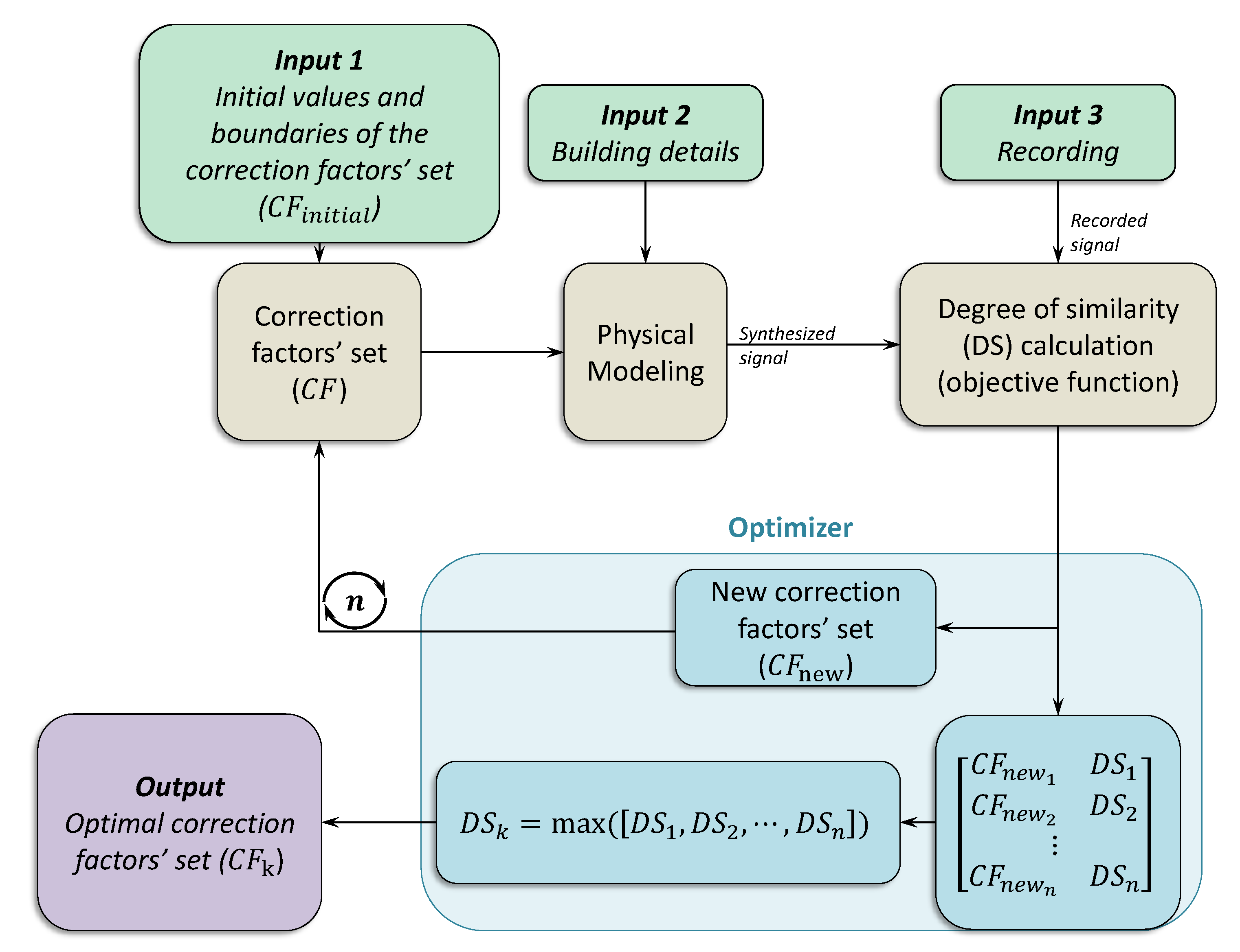
2. Method
3. Case Study: Recorder
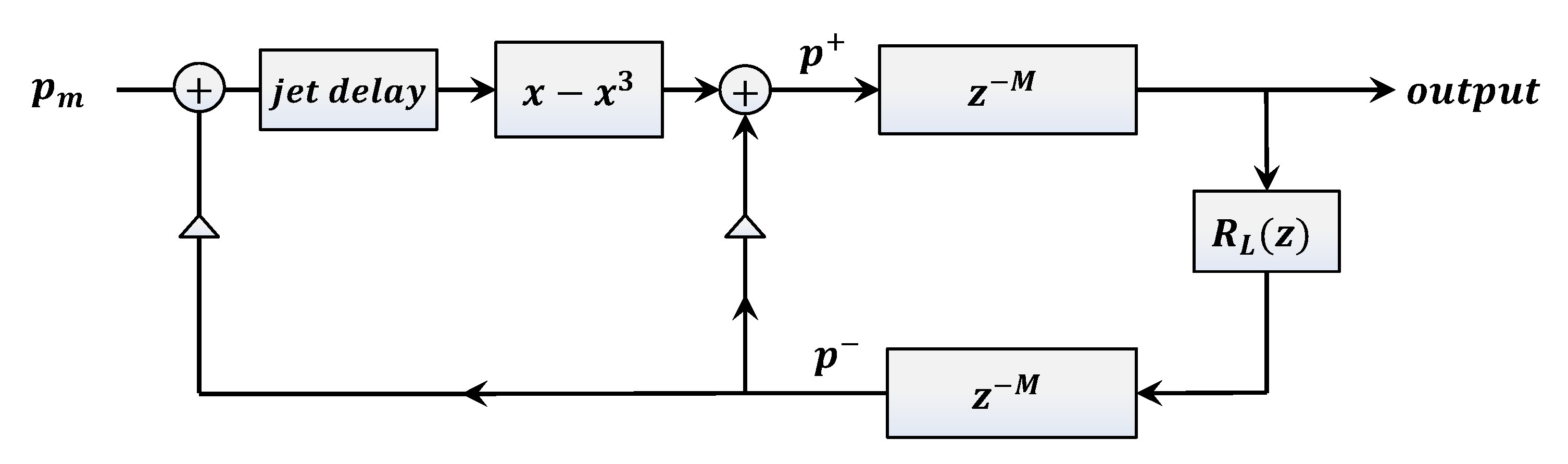
3.1. The Physical Model
3.2. Analysis by Synthesis Model
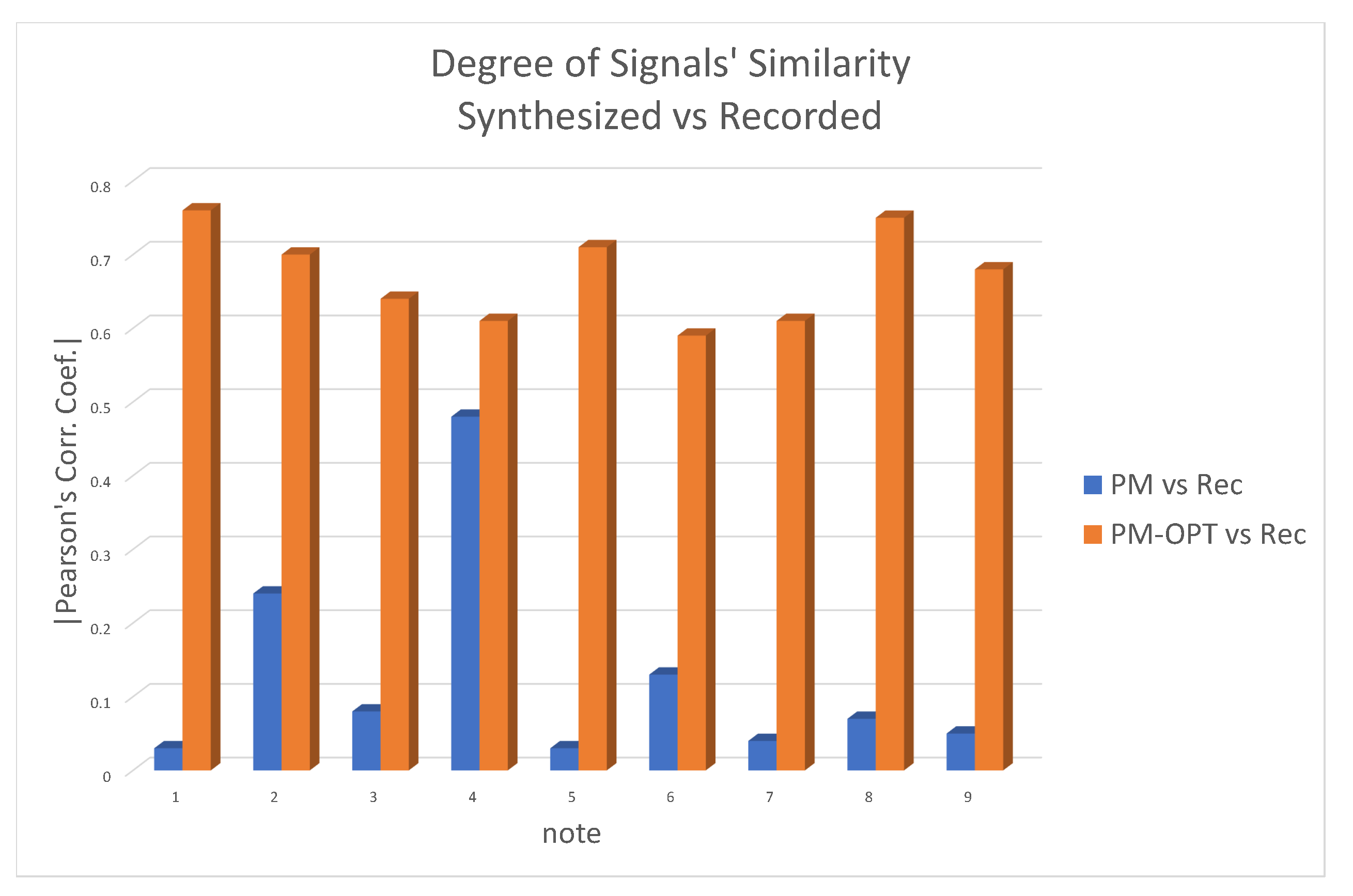
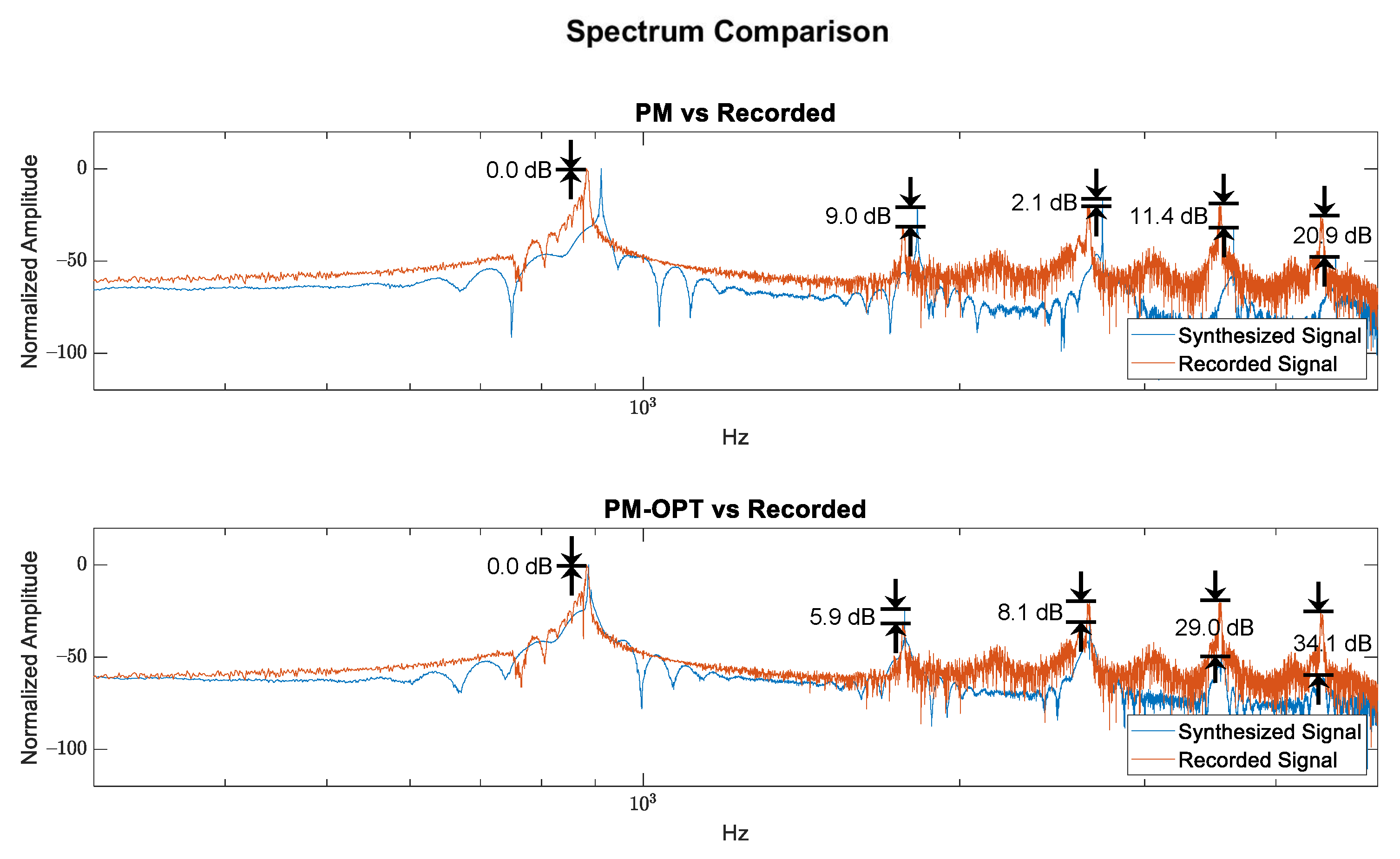
3.3. Results and Discussion
4. Conclusions
Author Contributions
Funding
Institutional Review Board Statement
Informed Consent Statement
Data Availability Statement
Conflicts of Interest
References
- Allen, A.; Raghubanshi, N. Aerophones in flatland: Interactive wave simulation of wind instruments. ACM Trans. Graph. 2015, 34, 134. [Google Scholar] [CrossRef]
- Schnell, N.; Battier, M. Introducing composed instruments, technical and musicological implications. In Proceedings of the 2002 Conference on New Interfaces for Musical Expression, Dublin, Ireland, 24–26 May 2002; Brazil, E., Ed.; National University of Singapore: Singapore, 2002; pp. 1–5. [Google Scholar]
- Hunt, A.; Wanderley, M.M.; Paradis, M. The importance of parameter mapping in electronic instrument design. J. New Music Res. 2003, 32, 429–440. [Google Scholar] [CrossRef]
- Bilbao, S. Direct simulation for wind instrument synthesis. In Proceedings of the 11th International Digital Audio Effects (DAFx-08) Conference, Espoo, Finland, 1–4 September 2008; pp. 1–8. [Google Scholar]
- Kontogeorgakopoulos, A.; Tzevelekos, P.; Cadoz, C.; Kouroupetroglou, G. Using the CORDIS-ANIMA Formalism for the Physical Modeling of the Greek Zournas Shawm. In Proceedings of the International Computer Music Conference (ICMC08), Belfast, UK, 24–29 August 2008; pp. 395–398. [Google Scholar]
- Tzevelekos, P.; Georgaki, A.; Kouroupetroglou, G.T. HERON: A Zournas Digital Virtual Musical Instrument. In Proceedings of the 3rd ACM International Conference on Digital Interactive Media in Entertainment and Arts (DIMEA), Athens, Greece, 10–12 September 2008; pp. 325–359. [Google Scholar] [CrossRef]
- Tzevelekos, P.; Perperis, T.; Kyritsi, V.; Kouroupetroglou, G. A Component-Based Framework for the Development of Virtual Musical Instruments Based on Physical Modeling. In Proceedings of the 4th Sound and Music Computing Conference, Lefkada, Greece, 11–13 July 2007; Spyridis, C., Georgaki, A., Kouroupetroglou, G., Anagnostopoulou, C., Eds.; National and Kapodistrian University of Athens: Athens, Greece, 2007; pp. 30–37. [Google Scholar]
- Pfeifle, F.; Bader, R.M. Real-Time Finite-Difference Method Physical Modeling of Musical Instruments Using Field-Programmable Gate Array Hardware. J. Audio Eng. Soc. 2015, 63, 1001–1016. [Google Scholar] [CrossRef]
- Smith, J.O., III. Viewpoints on the history of digital synthesis. In Proceedings of the International Computer Music Conference (ICMC 1991), Montreal, QC, Canada, 16–20 October 1991; pp. 1–10. [Google Scholar]
- Beauchamp, J.W. Analysis and Synthesis of Musical Instrument Sounds. In Analysis, Synthesis, and Perception of Musical Sounds. Modern Acoustics and Signal Processing; Beauchamp, J.W., Ed.; Springer: New York, NY, USA, 2007; pp. 1–89. [Google Scholar] [CrossRef]
- Smith, J.O., III. Physical Modeling Using Digital Waveguides. Comput. Music J. 1982, 16, 74–91. [Google Scholar] [CrossRef]
- Scavone, G. Delay-Lines and Digital Waveguides. In Springer Handbook of Systematic Musicology; Bader, R., Ed.; Springer: Berlin/Heidelberg, Germany, 2018; pp. 259–272. [Google Scholar] [CrossRef]
- Carpenter, T.G.F. Developing an Audio Unit Plugin Using a Digital Waveguide Model of a Wind Instrument. Master’s Thesis, Acoustics and Music Technology, University of Edinburgh, Edinburgh, UK, 2012. [Google Scholar]
- Smith, J.O. Digital waveguide architectures for virtual musical instruments. In Handbook of Signal Processing in Acoustics; Havelock, D., Kuwano, S., Vorländer, M., Eds.; Springer: New York, NY, USA, 2008; pp. 399–417. [Google Scholar] [CrossRef] [Green Version]
- Scavone, G.P. An Acoustic Analysis of Single-Reed Woodwind Instruments with an Emphasis on Design and Performance Issues and Digital Waveguide Modeling Techniques. Ph.D. Thesis, Stanford University, Stanford, CA, USA, 1997. [Google Scholar]
- Fletcher, N.H.; Rossing, T.D. The Physics of Musical Instruments, 1st ed.; Springer: New York, NY, USA, 1991; pp. 449–454. [Google Scholar]
- Cook, P.R. A meta-wind-instrument physical model, and a meta-controller for real-time performance control. In Proceedings of the International Computer Music Conference, San Jose, CA, USA, 14–18 October 1992; Michigan Publishing: Ann Arbor, MI, USA, 1992; pp. 273–276. [Google Scholar]
- Fletcher, N.H. Air flow and sound generation in musical wind instruments. Ann. Rev. Fluid Mech. 1979, 11, 123–146. [Google Scholar] [CrossRef] [Green Version]
- Wang, S. Wavelength and end correction in a recorder. ISB J. Phys. 2009, 3, 1–5. [Google Scholar]
- Wolfe, J. The acoustics of woodwind musical instruments. Acoust. Today 2018, 14, 50–56. [Google Scholar]
- Benesty, J.; Chen, J.; Huang, Y.; Cohen, I. Pearson correlation coefficient. In Noise Reduction in Speech Processing; Springer Topics in Signal Processing; Benesty, J., Kellermann, W., Eds.; Springer: Berlin/Heidelberg, Germany, 2009; Volume 2, pp. 1–4. [Google Scholar] [CrossRef]
- Singer, S.; Nelder, J. Nelder-mead algorithm. Scholarpedia 2009, 4, 2928. [Google Scholar] [CrossRef]
- Luersen, M.A.; Le Riche, R. Globalized Nelder–Mead method for engineering optimization. Comput. Struct. 2004, 82, 2251–2260. [Google Scholar] [CrossRef]
- Van Laarhoven, P.J.M.; Aarts, E.H.L. Simulated annealing. In Simulated Annealing: Theory and Applications; Van Laarhoven, P.J.M., Aarts, E.H.L., Eds.; Springer: Dordrecht, The Netherlands, 1987; pp. 7–15. [Google Scholar] [CrossRef]
- Kirkpatrick, S.; Gelatt, C.D.; Vecchi, M.P. Optimization by simulated annealing. Science 1983, 220, 671–680. [Google Scholar] [CrossRef] [PubMed]
- Polychronopoulos, S.; Memoli, G. Acoustic levitation with optimized reflective metamaterials. Sci. Rep. 2020, 10, 4254. [Google Scholar] [CrossRef] [PubMed] [Green Version]
- Bakogiannis, K.; Polychronopoulos, S.; Marini, D.; Terzēs, C.; Kouroupetroglou, G.T. ENTROTUNER: A computational method adopting the musician’s interaction with the instrument to estimate its tuning. IEEE Access 2020, 8, 53185–53195. [Google Scholar] [CrossRef]
- Fastl, H.; Zwicker, E. Psychoacousticss, 3rd ed.; Springer: Berlin/Heidelberg, Germany, 2007. [Google Scholar] [CrossRef] [Green Version]


| Note | Recorded Signals Frequency (Hz) | ||||
|---|---|---|---|---|---|
| Fundamental | 1st Overtone | 2nd Overtone | 3rd Overtone | 4th Overtone | |
| 1 | 522 | 1046 | 1568 | 2090 | 2614 |
| 2 | 591 | 1183 | 1774 | 2365 | 2957 |
| 3 | 661 | 1322 | 1982 | 2644 | 3305 |
| 4 | 721 | 1439 | 2160 | 2883 | 3604 |
| 5 | 781 | 1560 | 2347 | 3131 | 3901 |
| 6 | 883 | 1767 | 2659 | 3536 | 4414 |
| 7 | 1003 | 2005 | 3011 | 4013 | 5017 |
| 8 | 1117 | 2334 | 3352 | 4469 | 5586 |
| 9 | 1213 | 2428 | 3642 | 4855 | 6070 |
| Note | Synthesized Signals Frequency (Hz) | |||||||||
|---|---|---|---|---|---|---|---|---|---|---|
| Fundamental | 1st Overtone | 2nd Overtone | 3rd Overtone | 4th Overtone | ||||||
| PM | PM-OPT | PM | PM-OPT | PM | PM-OPT | PM | PM-OPT | PM | PM-OPT | |
| 1 | 511 | 523 | 1022 | 1045 | 1533 | 1568 | 2044 | 2091 | 2555 | 2613 |
| 2 | 594 | 591 | 1188 | 1183 | 1782 | 1774 | 2376 | 2365 | 2970 | 2957 |
| 3 | 668 | 661 | 1337 | 1322 | 2005 | 1982 | 2673 | 2643 | 3342 | 3304 |
| 4 | 722 | 721 | 1444 | 1441 | 2165 | 2162 | 2887 | 2883 | 3609 | 3603 |
| 5 | 824 | 781 | 1649 | 1563 | 2473 | 2344 | 3297 | 3125 | 4122 | 3906 |
| 6 | 912 | 884 | 1823 | 1767 | 2735 | 2651 | 3647 | 3538 | 4559 | 4415 |
| 7 | 1013 | 1003 | 2027 | 2007 | 3040 | 3010 | 4054 | 4013 | 5068 | 5017 |
| 8 | 1197 | 1111 | 2394 | 2222 | 3592 | 3333 | 4789 | 4443 | 5986 | 5554 |
| 9 | 1222 | 1214 | 2444 | 2428 | 3666 | 3622 | 4888 | 4856 | 6110 | 6073 |
| Note | Deviation of Synthesized Signals from the Recorded Signals (in Cents) | |||||||||||
|---|---|---|---|---|---|---|---|---|---|---|---|---|
| Fundamental | 1st Overtone | 2nd Overtone | 3rd Overtone | 4th Overtone | Partials Average | |||||||
| PM | PM-OPT | PM | PM-OPT | PM | PM-OPT | PM | PM-OPT | PM | PM-OPT | PM | PM-OPT | |
| 1 | 37 | 3 | 40 | 2 | 39 | 0 | 39 | 1 | 39 | 1 | 39 | 1 |
| 2 | 9 | 0 | 7 | 0 | 8 | 0 | 8 | 8 | 0 | 8 | 0 | |
| 3 | 18 | 0 | 20 | 0 | 20 | 0 | 19 | 1 | 19 | 1 | 19 | 0 |
| 4 | 2 | 0 | 6 | 2 | 4 | 2 | 2 | 0 | 2 | 1 | 3 | 1 |
| 5 | 93 | 0 | 96 | 3 | 91 | 2 | 89 | 3 | 95 | 2 | 93 | 2 |
| 6 | 56 | 2 | 54 | 0 | 49 | 5 | 54 | 1 | 56 | 0 | 54 | 2 |
| 7 | 17 | 0 | 19 | 2 | 17 | 1 | 18 | 0 | 18 | 0 | 18 | 1 |
| 8 | 120 | 9 | 120 | 9 | 120 | 10 | 120 | 10 | 120 | 10 | 120 | 10 |
| 9 | 13 | 1 | 11 | 0 | 12 | 10 | 11 | 0 | 11 | 1 | 12 | 2 |
| Total average absolute deviation | 41 | 2 | ||||||||||
Publisher’s Note: MDPI stays neutral with regard to jurisdictional claims in published maps and institutional affiliations. |
© 2021 by the authors. Licensee MDPI, Basel, Switzerland. This article is an open access article distributed under the terms and conditions of the Creative Commons Attribution (CC BY) license (https://creativecommons.org/licenses/by/4.0/).
Share and Cite
Bakogiannis, K.; Polychronopoulos, S.; Marini, D.; Kouroupetroglou, G. Audio Enhancement of Physical Models of Musical Instruments Using Optimal Correction Factors: The Recorder Case. Appl. Sci. 2021, 11, 6426. https://doi.org/10.3390/app11146426
Bakogiannis K, Polychronopoulos S, Marini D, Kouroupetroglou G. Audio Enhancement of Physical Models of Musical Instruments Using Optimal Correction Factors: The Recorder Case. Applied Sciences. 2021; 11(14):6426. https://doi.org/10.3390/app11146426
Chicago/Turabian StyleBakogiannis, Konstantinos, Spyros Polychronopoulos, Dimitra Marini, and Georgios Kouroupetroglou. 2021. "Audio Enhancement of Physical Models of Musical Instruments Using Optimal Correction Factors: The Recorder Case" Applied Sciences 11, no. 14: 6426. https://doi.org/10.3390/app11146426
APA StyleBakogiannis, K., Polychronopoulos, S., Marini, D., & Kouroupetroglou, G. (2021). Audio Enhancement of Physical Models of Musical Instruments Using Optimal Correction Factors: The Recorder Case. Applied Sciences, 11(14), 6426. https://doi.org/10.3390/app11146426