1. Introduction
Wellness indicates the state or condition of being in good physical and mental health. According to the World Health Organization, health should be defined as a state of complete physical, mental, and social wellness, and not merely as the absence of disease and infirmity [
1].
Stress is a common state of emotional strain that plays a crucial role in everyday quality of life with a significant impact on the wellness state of a person. This state consists of several complementary and interacting components (i.e., cognitive, affective, and psycho-physiological). Furthermore, chronic stress carries a wide range of health-related diseases, including cardiovascular diseases, cerebrovascular diseases, diabetes, and immune deficiencies [
2,
3]. Due to the adverse effects of stress in our daily life, stress monitoring and management has been receiving an increasing attention in healthcare and wellness research [
4]. As a matter of fact, stress is recognized as a major risk factor for most non-communicable diseases and its evaluation is crucial for defining individual wellness.
Stress induces anomalous responses of the Autonomic Nervous Systems (ANS) which is a main actor in stress counteraction [
5,
6]. In particular, the activation of the sympathetic nervous system might be accompanied by many physical reactions, such as increasing the heart rate and blood supply to muscles, activating sweat glands, and increasing respiratory rate.
As to stress monitoring, several physiological signals and indicators provide important clues about individual status. Heart rate (HR) and heart rate variability (HRV) are crucial indicators of the psychophysical status of an individual and are useful clues for detecting risky conditions. The HR varies according to the body’s physical needs, changes being observed in a variety of conditions including physical exercise, sleep, anxiety, stress, illness, and assumption of drugs. Monitoring the heart rate is therefore important in both normal and disease conditions. The HRV is an index of the adaptation of the heart to circumstances by detecting and readily responding to unpredictable stimuli. The HRV is mainly modulated by the sympathetic and parasympathetic components of the autonomic nervous system [
7]. Beside alterations related to cardiac diseases [
8], HRV is an important measure of mental stress and, coupled with the HR, is commonly used to monitor individual wellness in behavioral research [
9]. The gold standard for HR and HRV assessment is ECG recording that allows the fine localization of heart beats [
10]. In recent years, several methods have been studied to allow the non-contact measurement of HR and HRV, including HR from speech [
11], thermal imaging [
12], microwave Doppler effect [
13], and imaging photoplethysmography (iPPG) [
14,
15,
16,
17]. The latter approach could greatly simplify data acquisition, making measurement easily available in non-clinical scenarios (e.g., driver monitoring [
14], human–machine interaction monitoring [
18]). According to our previous experience [
19], iPPG can offer a valid alternative to standard PPG.
Respiratory rate (RR) carries important information on a person’s health condition and physiological stability, an abnormal respiratory rate being a strong illness indicator [
20]. In particular, respiratory rate increases significantly under stressful situations [
21]. Current methods to collect respiration data include the use of respiration belts, measurement of impedance through ECG electrodes, spirometers, or visual observation/counting. These techniques have drawbacks that limit the frequency and convenience of the respiratory monitoring. The large diffusion of wearable devices has stimulated interest in monitoring athlete training, with the aim of maximizing performance, and minimizing the risk of injury and illness. In these field, chest belts are a common choice. It worth mentioning that respiratory rate too could be monitored by imaging ([
22,
23,
24]).
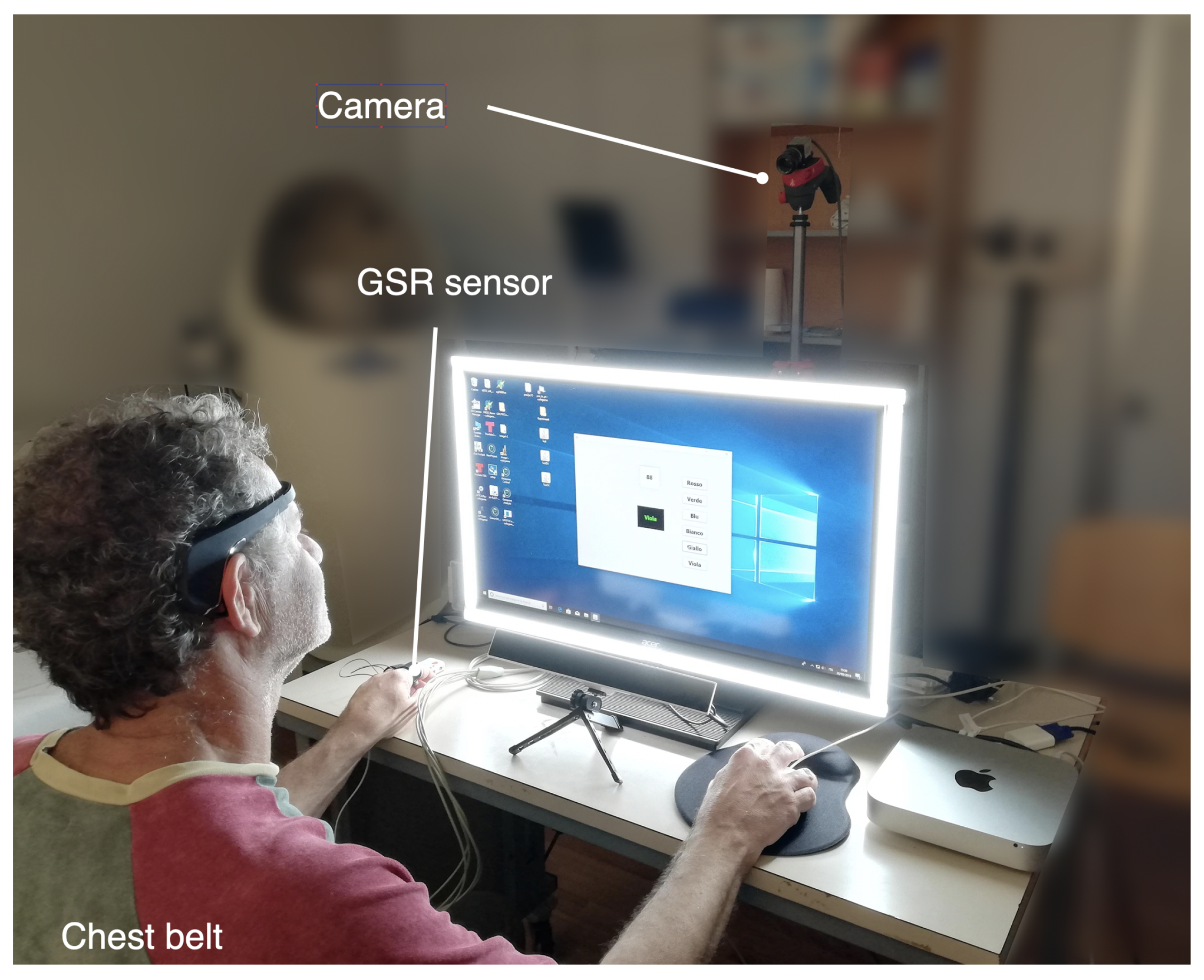
Galvanic skin response (GSR) is sensitive to many different stimuli (strong emotion, a startling event, pain, exercise, deep breathing, a demanding task, cognitive workload, and stressing stimulation) and identifying the primary cause of a particular skin-conductivity response may be hard. Anyway, a lot of different studies reported that the electrodermal response represents an adequate measure for stress-related sympathetic activation [
25]. GSR can be measured by different methods. In general, GSR sensor measures the real-time skin conductance which is related to the sweat gland activity depending on emotional response and environmental condition [
26]. GSR is typically acquired in hand fingers.
In recent years, the interest of the scientific community has progressively expanded toward multi-sensing technologies able to integrate different signals and build effective monitoring system useful to detect dangerous conditions and driving coping actions [
27]. In particular, machine learning paradigms looks very promising, and their application is an active field of investigation [
28,
29,
30].
A common framework of most studies on stress detection/monitoring is the evaluation of response to maximal (or intense) stress. This provides significant details on the individual capability to react to severe stress. On the other hand, maximal activation is not the most common experience in everyday life. People usually face a wide spectrum of stressors implying a variety of activations both positive and negative.
In this work, we focus on the impact of mild stimulations which can be somehow comparable to usual conditions that everyone can deal with in daily life. The aim is to set up a general platform useful to observe the individual status in routine setting (e.g., working in an office, driving a car) making it possible to design minimally obtrusive monitoring/testing procedures for detecting stress situations even in response to mild cognitive activation or other daily activities.
In the following we will report on the use of machine learning techniques for recognizing activation statuses with respect to resting conditions. To obtain a description of individual status, iPPG, respiratory waves and GSR signals are integrated at feature level. Our main aim is to build a flexible representation scheme able to capture the different facets of individual status, rather than implementing a rest/stress classification scheme. The reported usage of Kohonen map allows the representation of the individual status through a set of prototypes (weight vectors) learned from real data without supervision.
In next sections, after describing the used datasets (
Section 2) and the related harmonization/processing methodology adopted to derive a compact feature set from signals acquired in different conditions (
Section 3), we analyze the discriminating power of such a feature set (
Section 4) and describe the use of the Self-Organizing Map (SOM) to represent the status of an individual (
Section 5). Results are reported in
Section 6.
3. Dataset Harmonization and Analysis
For each subject, the MCA dataset included three blocks of data. The first block was 5 min long and contained the data acquired during the rest state. The other two blocks were 2 min and 3 min long respectively and contained data acquired during activation of Test A and B, respectively. For our aims, these two blocks were merged into a single 5-min window. In this way, each record contains two 5-min blocks.
To homogenize the data from the two datasets, all SRAD recordings were divided into non-overlapping blocks lasting five minutes. For each subject we had, on average, a 3–5 blocks representing the resting condition and about 9–11 blocks for driving periods. A total of 140 blocks, 39 at rest and 101 during driving was extracted.
Signals and data of both datasets were analyzed to extract a set
Y of 12 psychophysical features from ECG, video signal, RR, and GSR as summarized in
Table 1.
It is worth mentioning that data from auto-evaluation questionnaires are only available for MCA and, therefore, they were not considered for data analysis. In any case, all MCA subjects did not refer relevant stressing conditions both before, during, and after test.
3.1. MCA Dataset Analysis
The video signal was processed as described in [
19] to extract HR and HRV descriptors. In particular, blood volume pulses were detected by analyzing time peaks in video signals. The related time series provided the video tachogram used for HRV analysis. To remove possible artifacts, the inter beat intervals were analyzed by a variable-threshold non-causal algorithm [
37]. Tachograms were analyzed both in time domain and in frequency domain. Concerning time domain, we calculated the average time between adjacent normal heartbeats (NN) and its standard deviation (SDNN). Concerning frequency domain, HRV description was based on power spectrum density (PSD), as estimated by the Lomb–Scargle periodogram. According to the standard definition of the HRV frequency bands, low frequency (LF) and high frequency (HF) were calculated as the area under the PSD curve corresponding from 0.04 Hz to 0.15 Hz and from 0.15 Hz to 0.4 Hz, respectively. The LF component reflects both sympathetic and parasympathetic actions, the HF component reflects parasympathetic action, and the LF/HF ratio is a measure of the sympatho/vagal balance.
The values of the median, the interquartile range, the minimum, and the maximum were calculated for the respiratory rate. RR waveforms were monitored to detect too long or too short leading to a rate outside a physiological range (8–25 bpm).
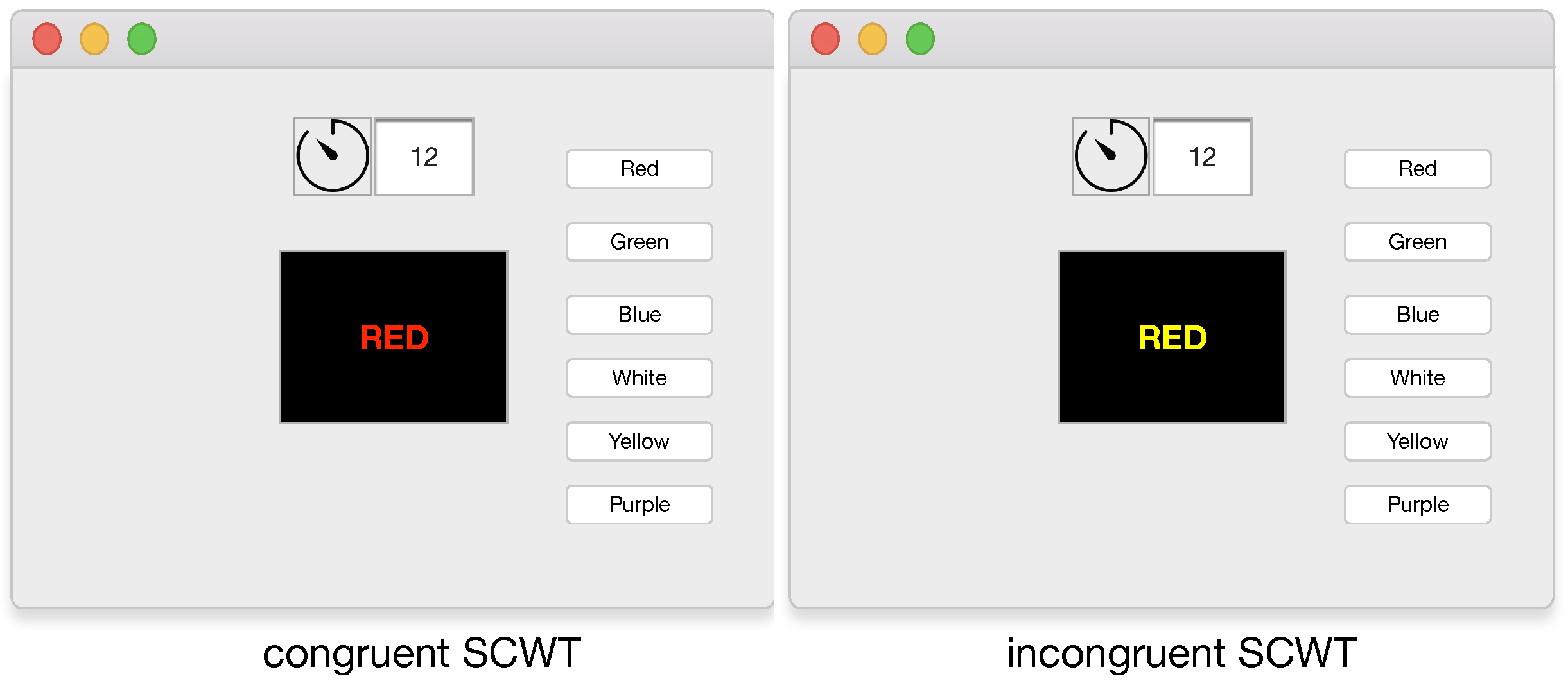
Concerning the galvanic skin response, the interfering mains frequency (50 Hz) was removed from the signal by a notch filter. Subsequently, the GSR signal was down sampled to 10 Hz. Then it was filtered through a mean filter spanning a 4 s window and a median filter spanning 8 s. To obtain the phasic component, the signal from the median filter was subtracted to the one from the mean filter. The number of peaks, the maximum peak amplitude, and the median peak value were calculated. A total of 20 blocks was then available from MCA: 10 in rest condition and 10 during SCWT.
3.2. SRAD Dataset Analysis
Due to incompleteness of data, seven SRAD subjects were excluded from the analysis, and a sub-group of 10 subjects with IDs 4, 5, 7, 8 , 9, 10, 11, 12, 15, and 16 was considered in this work. Only the signals common to MCA dataset were analyzed. They included: ECG, respiratory wave, and the GSR acquired on the palm of the hand. ECG signals were first pre-processed to detect QRS complexes by Pan-Tompkins algorithm [
38] and derive tachograms that were processed as in the case of MCA data. The respiratory rate (breaths per minute) was estimated from the respiratory wave by detecting and counting the signal peaks. The GSR was analyzed as previously described for the MCA dataset.
We wish to point out that 13 blocks of ECG recordings (10 at rest and 3 during driving) resulted corrupted and were not included in the analysis. A total of 127 blocks was therefore available from SRAD: 29 in rest condition and 98 during driving.
4. Feature Analysis and Activation Recognition
We have analyzed the Y feature set with respect to its capabilities to recognize resting states from activation ones, particular attention being paid to the relevance of the various features. To this end we investigated two complementary approaches: Sequential Forward Feature Selection (SFFS) and Auto-Encoder (AE) neural networks.
SFFS is a well-established search algorithm whose advantages and limits are well known [
39]. In particular, SFFS is known to work nicely, though non-optimally, for spaces with moderate dimension [
40]. Therefore, though more sophisticated techniques exist, we adopted SFFS as reasonable trade-off between simplicity and expected accuracy.
Simple feature selection is based on the use of a possibly optimal subset of available features, and may hinder the correlation among features. During the feature selection process, dimensionality reduction is usually achieved by completely discarding some dimensions, which inevitably lead to loss of information. However, sample data in high-dimensional space generally cannot diffuse uniformly in the whole space; they actually lie in a low-dimensional manifold embedded in high-dimensional space, the dimension of the manifold being called the intrinsic dimensionality of the data [
41]. Therefore, we explored an alternative approach based on AEs. They provide a sort of non-linear generalization of principal component analysis [
42]. AEs are largely employed in different machine learning applications and provide a modern non-supervised framework to assess the intrinsic dimensionality of data space based on neural networks that learn to output an optimal reconstruction of the input.
Methods were implemented in MATLAB using ad hoc scripts.
4.1. Sequential Forward Feature Selection
As summarized in Algorithm 1 SFFS is an iterative search algorithm aiming to find the best subset including
features of the original
n-dimensional set
Y according to the predefined criterion
J. At first the best single feature optimizing a predefined criterion is individuated. Afterward, the same criterion is optimized using pairs of features, pairs being generated by sequentially adding to the previous best single feature one of the remaining features. The best couple of features is so defined. Next, triplets of features are formed using one of the remaining features and the previous best couple. This procedure continues until
K features are found.
| Algorithm 1: Sequential Forward Feature Selection |
![Applsci 11 06381 i001]() |
The process was implemented using the MATLAB sequentialfs function which selects a subset of features from the data matrix that best predict the data by sequentially selecting features until there is no improvement in prediction. Prediction was implemented by Linear Discriminant Analysis (LDA) [
43]. For each candidate feature subset,
sequentialfs performs 10-fold cross-validation by repeatedly training and testing a model (in our case the LDA classifier) with different training and test subsets.
As
sequentialfs randomly splits the initial dataset to implement 10-fold cross-validation, the feature selection process can yield to different results depending on the run. This is true for both the number of selected features and which features are selected. To analyze this effect,
sequentialfs was run 1000 times. For each run, we recorded the features selected by the procedure and the order in which they were selected. In addition, we set up a scoring system to properly weigh the relevance of the features. Specifically, at each run, every selected feature received a score equal to its position in the selection process (e.g., 1 for the first one, 3 for the third one). The features that were not selected were given a conventional score of 12. The process was repeated for every run and the scores for each run were summed up. By doing so, a final score of 1000 would indicate a feature selected as the first one in all runs. A feature with a final score of 12,000 would be a feature never selected by the method. The method was trained using the SRAD, while MCA data were used as independent test set. Related results are reported in
Section 6, where the behavior of k-means clustering is also discussed.
4.2. Auto-Encoder Neural Networks
An auto-encoder neural network was applied to the SRAD dataset. This was designed as a feed-forward neural network with 12 input units, a single hidden layer with logistic activation, and an output layer with 12 units. The hidden layer had several units variable from 1 to 12.
The network was trained to reconstruct the input pattern by minimizing the
loss function using the scaled conjugate gradient descent algorithm [
44] with a maximum number of epochs set to 1000.
To optimize data usage and reduce the risk of over-fitting, a training scheme based on 5-fold cross-validation. Twelve AE models were obtained, each with a different number of hidden units ranging from 1 to 12.
Using the feature sets generated by the auto-encoder, we trained a family of LDA classifiers to recognize driving periods from rest ones in the SRAD data. This process generated 12 classification models each of them using several features ranging from 1 to 12.
In
Section 6, accuracy of LDA classifiers in predicting the activation level based on AE features is reported.
5. Representation of Activation Status in SOM Space
Up to now we have considered the discrimination of resting statuses from activity-related ones, a task relevant for monitoring and possibly advising a person against risky conditions. As a matter of fact, a sharp dichotomization between activation and rest is rather arbitrary and dependent on the subject. In facts, stress responses are largely variable among individuals and, for an individual, they vary with time. It is, therefore, not surprising that for a given subject, a set of feature values can relate to a possible activation status, while for another subject similar values can relate to a different condition. On the other hand, labels used for training are defined by the presence/absence of stimulation which, in general, produces a different response depending on the subject. Therefore, we decided to explore unsupervised machine learning paradigms which do not need a priori data labeling. In particular, we resorted to investigate the use of Kohonen SOM which can build accurate, but low-dimensional, topology preserving-maps of the input data space [
45]. This means that similar inputs data tend to excite neighboring units in the map.
The map space is defined beforehand, usually as a finite two-dimensional region where a set of nodes is arranged in a regular grid.
Each node is fed by input data
via a weight vector
. For a given input
, the output of the network is defined by the best matching (or winning) unit
obtained by:
The weight represents the network response and is a point in data space. In this way, the SOM maps the high-dimensional input space to the low-dimensional network space.
During training, nodes in the map space stay fixed, while their weight vectors are moved toward the input data without spoiling the topology induced from the map space. During a training epoch all input patterns are presented to the network. For each pattern, the weight of
unit and neighboring units are adapted according to a predefined neighborhood function
(Gaussian is a common choice for
h). In this work we adopted the batch version of the SOM adaptation algorithm [
45] leading to the adaptation rule:
Equation (
2) ensures a faster convergence and provide more stable results with respect to stochastic adaptation. After training, SOM can build accurate topographic representation of the input space catching significant details including data clustering. In particular, each weight vector ca be viewed as a prototype in data space as it tends to respond to a set of “near” input points.
Using the MATLAB Neural Network package, we have analyzed 2D maps of varying dimensions, from 3 × 3 to 6 × 6 units. Networks were trained using the SRAD dataset. The obtained maps were tested using the MCA dataset.
6. Results
Data were analyzed from different viewpoints including feature analysis and selection and their ability to describe and recognize rest from activation statuses. Given the limited sample size of MCA dataset we decide to use SRAD data as development set and MCA data as test set.
6.1. SFFS Analysis
Results of the feature selection process are summarized in
Table 2 where features are ranked according to the SFFS score and selection frequency is also reported. In particular, the median RR was selected in all runs, and is constantly the most relevant single feature. This suggests that it carries a significant piece of information, irrespective of how the data are split between training and test set. The number of GSR peaks obtains the second score in the process, being selected in almost 99% of the runs.
After the first two features, we observed a marked drop in the score. Indeed, LF/HF (the feature with the third best score, i.e., >9200) was selected in 34% of the runs only. Similar results were observed for the RR interquartile range and NN. Finally, all other features have scores that are very close to the maximum (>10,000) to end up with the last one (the maximum RR) never being selected by the process.
Table 3 shows values for the two most relevant features for all subjects of SRAD used in this work. Analogous data are reported for MCA in the
Table 4.
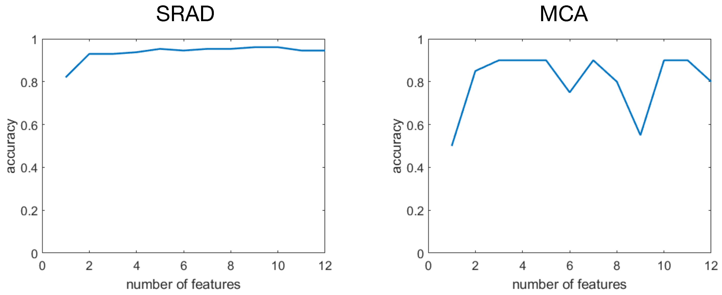
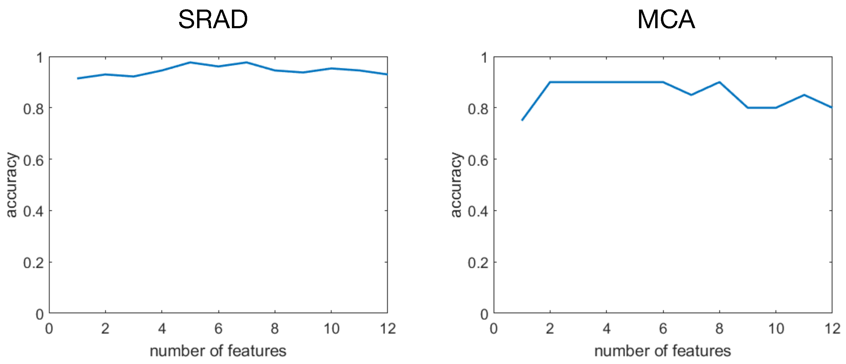
In
Figure 3 we plot the accuracy of LDA classifier obtained on the SRAD dataset with different numbers of features according to SFFS ranking. A similar plot is also given for MCA as test set. For SRAD the accuracy amounts at about 93% for a single feature rising to about 98% with two features with no further significant changes using the remaining features. For the MCA data we observe a rapid increase to about 90% with two features, fluctuations being present when using more than six features.
6.2. AE Features
In general, the observed accuracy of AE features resulted high (>90%), with the worst performance (about
) obtained when a single feature was available (
Figure 4). When two (or more) features were employed, the accuracy fluctuated around 93–95%. Therefore using more than two AE features did not significantly improve discrimination capabilities. Indeed, a maximal accuracy of (about
) was already met using two features.
When each of the 12 models were tested on the MCA dataset, results were found to be affected by a larger variability (
Figure 4). With a single feature, the accuracy is
(chance level). However, also in this case, using two features produces a substantial accuracy boosting. This reached its maximum with three features (at around
). The inclusion of additional features results in accuracy fluctuation about lower values.
To sum up, both SFFS and AE support the finding that two features may be sufficient to reliably recognize activation statuses.
6.3. Data Clustering
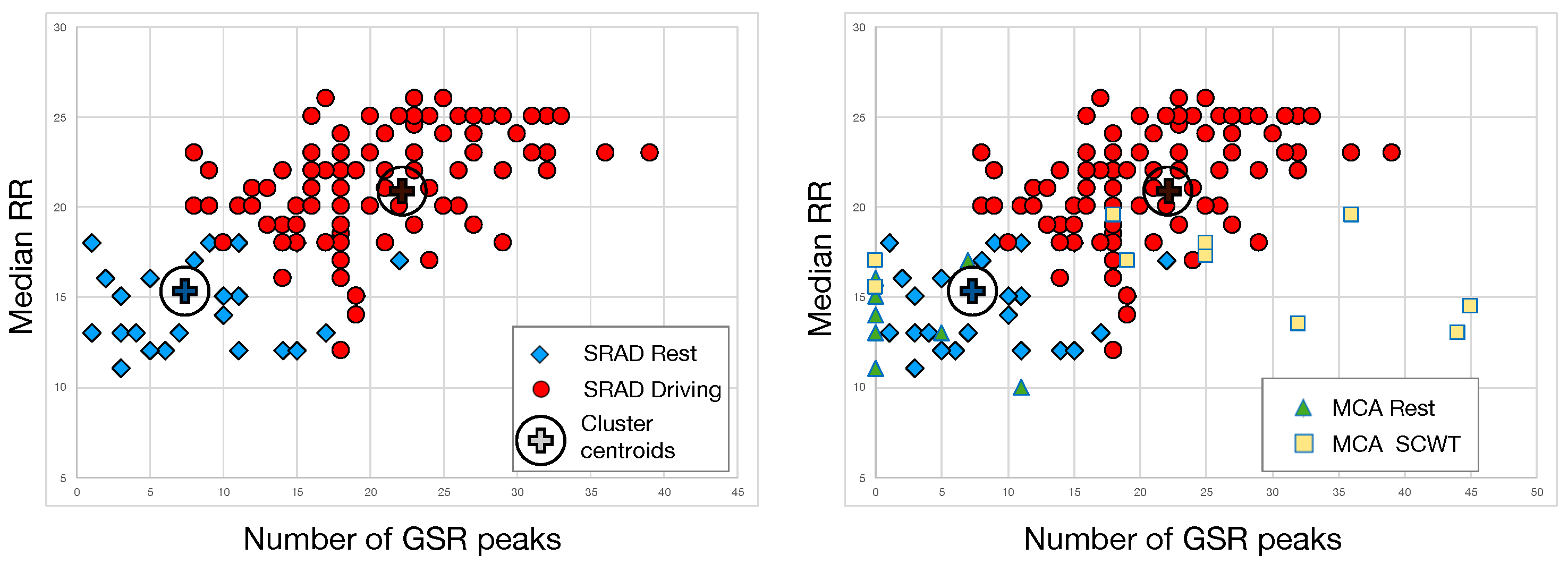
According to the results of the selection process, the best features were identified as the median RR and the number of GSR peaks. We have further investigated the joint use of these features with respect to their capability to cluster the data space. To this end, we partitioned SRAD data in two cluster using standard k-means algorithm as provided in MATLAB. Clustering (see
Figure 5) was correlated with the dataset labels (either rest or driving). K-means clustering led to an 87.9% recognition rate for the rest state and a 92.3% recognition rate for the driving state. As shown in
Table 5, the overall classification accuracy was 89.4%.
It is worth mentioning that using the same cluster centroids for MCA data we found a 90% rate of correct classification (
Figure 5). By taking a closer look at these results, we found that
classification accuracy was not achieved as the algorithm failed to recognize the activation state of the two non-naïve subjects. Actually, they have had significant previous experience with the SCWT.
To better understand what could have been the contribution of additional features, we repeated the same process using other features. However, performance of k-means clustering deviated significantly from rest/activation data labeling.
Finally, we wish to point out that k-means was repeated 1000 times with random cluster initialization: we observed changes in final centroid position in less than of cases. However, even in these cases, displacement of cluster centroids was quite limited. Indeed, we observed a change in coordinates of the total range of the feature space.
6.4. Self-Organizing Maps
We have trained a set of two-dimensional SOMs with several units varying from to . We did not consider larger maps due the limited dataset size. Maps were trained on the SRAD dataset. For each map size, training was run ten times with random weight initialization. Apart changes in map orientation, no relevant difference was detected inside each run.
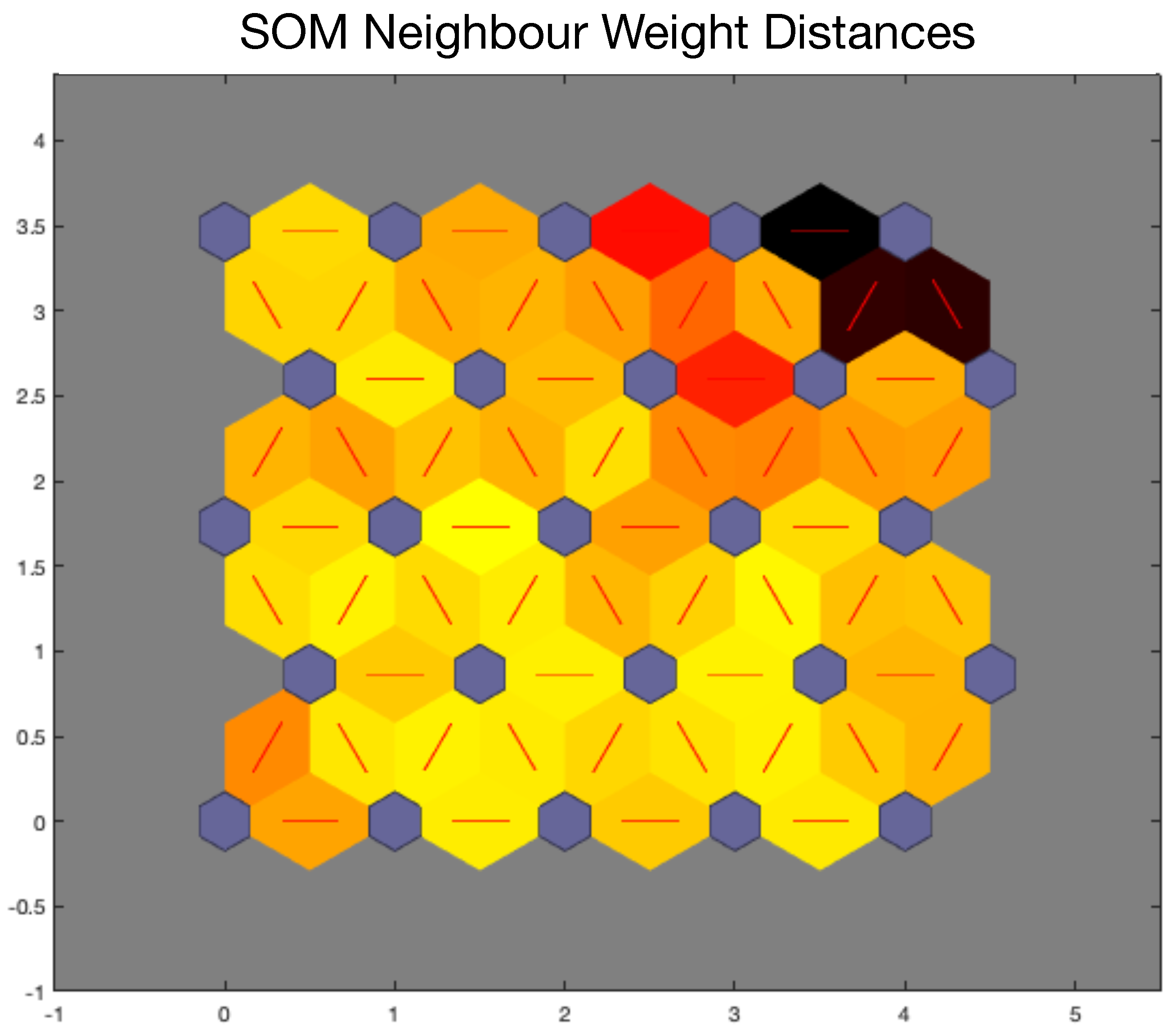
As we are interested in the topographic representation produced by SOMs, we have analyzed each map with respect to the distance between weights of neighboring units (the so-called U-map), and the distribution in the network space of each weight dimension (weight-plane maps). In addition, to explore the semantic role of unit activation we analyzed the distribution of data labels in network space (categorical hit maps). Since the results do not vary significantly with the number of units, to ease readability, we show only data for SOM.
Map distances in
Figure 6 suggest that the units in the right upper corner are rather apart from the other units that tend to be closer each other. This confirms previous data from feature selection and data clustering, and suggests that the data space can be partitioned into two highly structured clusters. It is worth noting that larger maps are expected to capture finer structural details of data as suggested by the comparison of the maps.
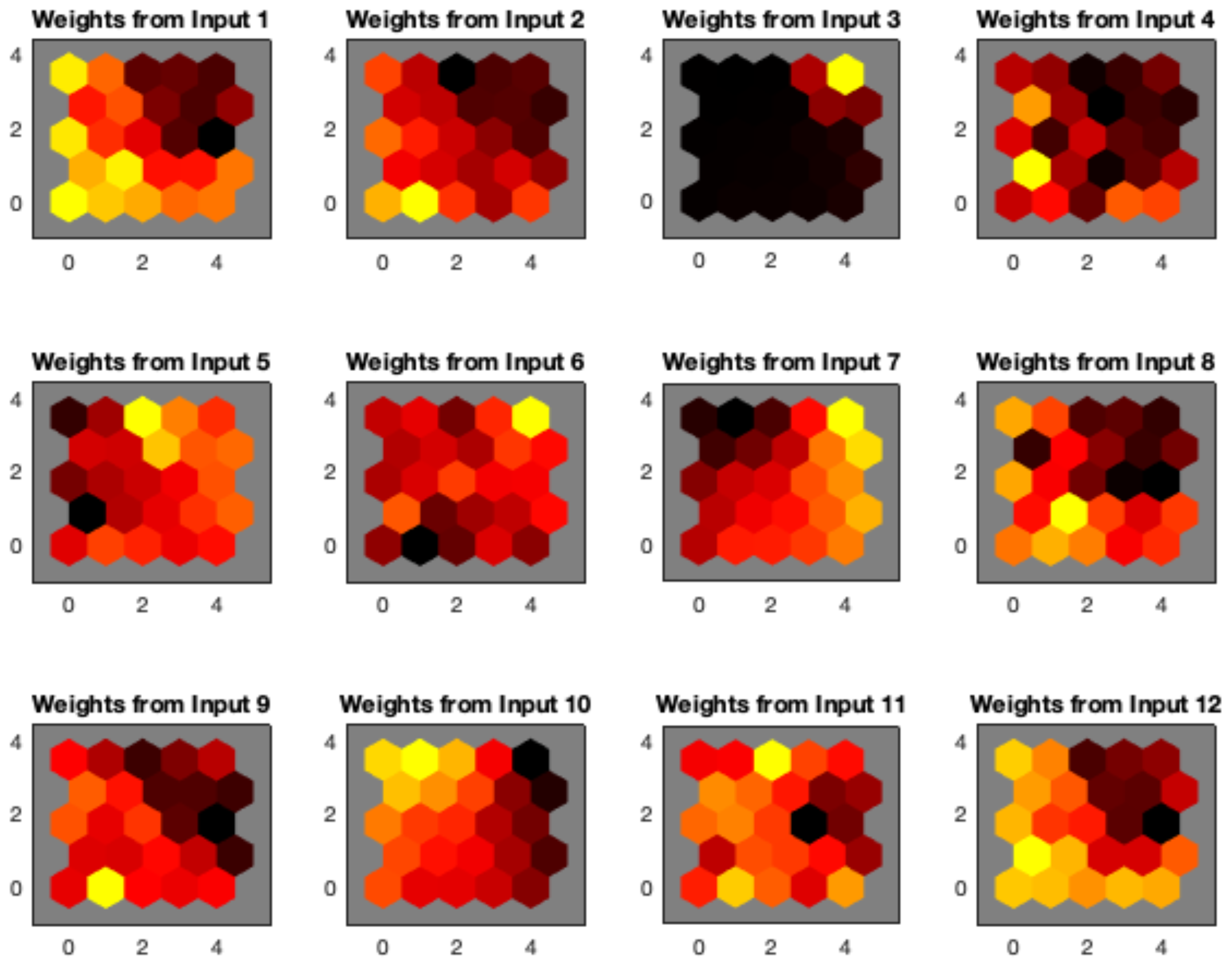
The distribution of SOM weights (
Figure 7) provides additional support to distance maps. In particular, spatial arrangement of weights looks consistent among different map sizes. In addition, several components (e.g., those corresponding to median RR, GSR peak number, LF/HF, NN, LF, and HF ) exhibit a well-defined spatial distribution. In particular, some of them such as the weights of median RR and GSR peak number can be related to the partition appearing the left upper part of the map.
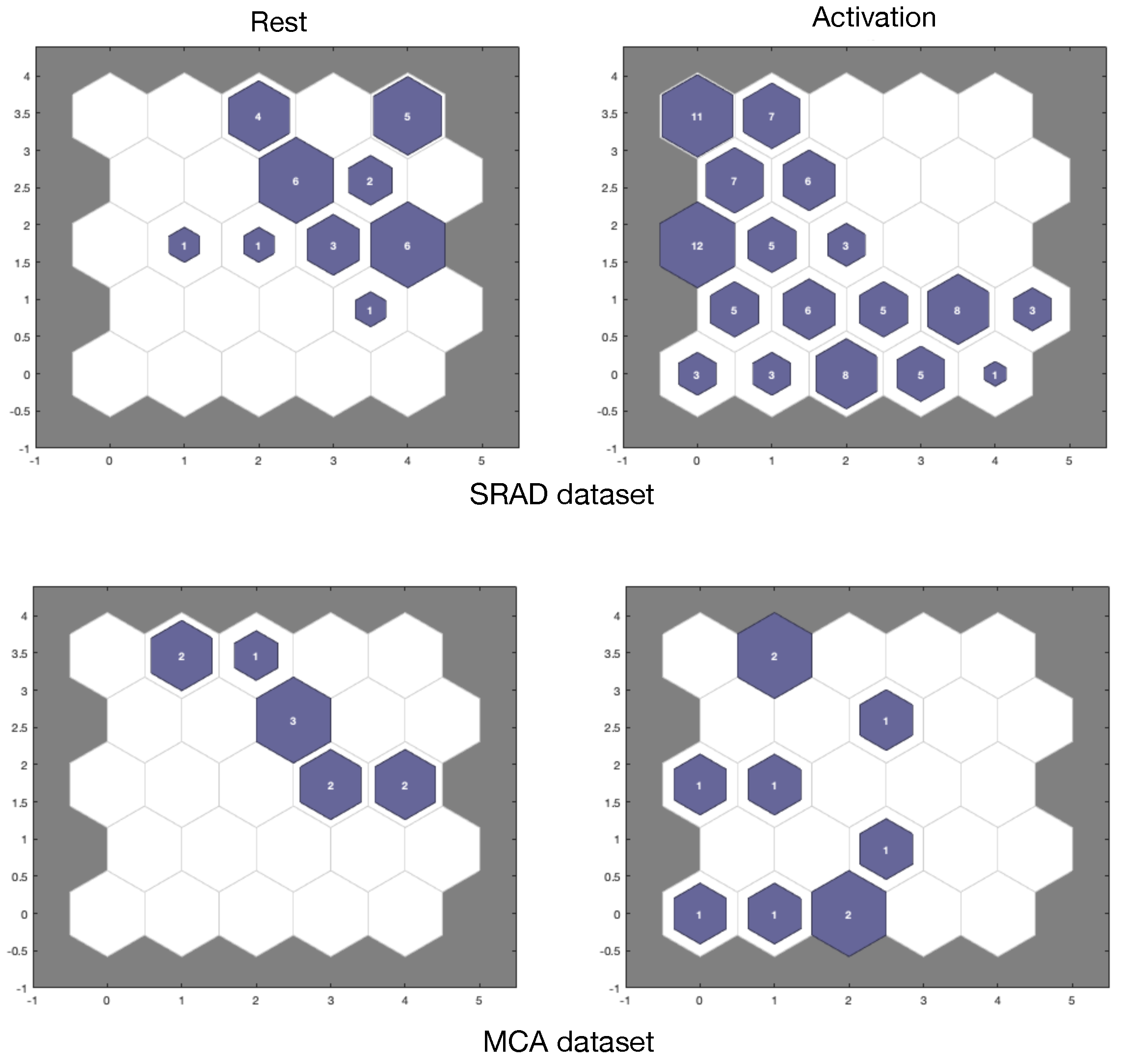
Categorical hit maps (top of
Figure 8) for the rest and activation labels of the SRAD dataset show a rather neat distinction among the two categories: only a few units respond simultaneously to both rest and activation data. In the bottom part of
Figure 8, we report the hit maps for rest and activation categories of MCA dataset. These maps exhibit a behavior similar to the case of SRAD data.
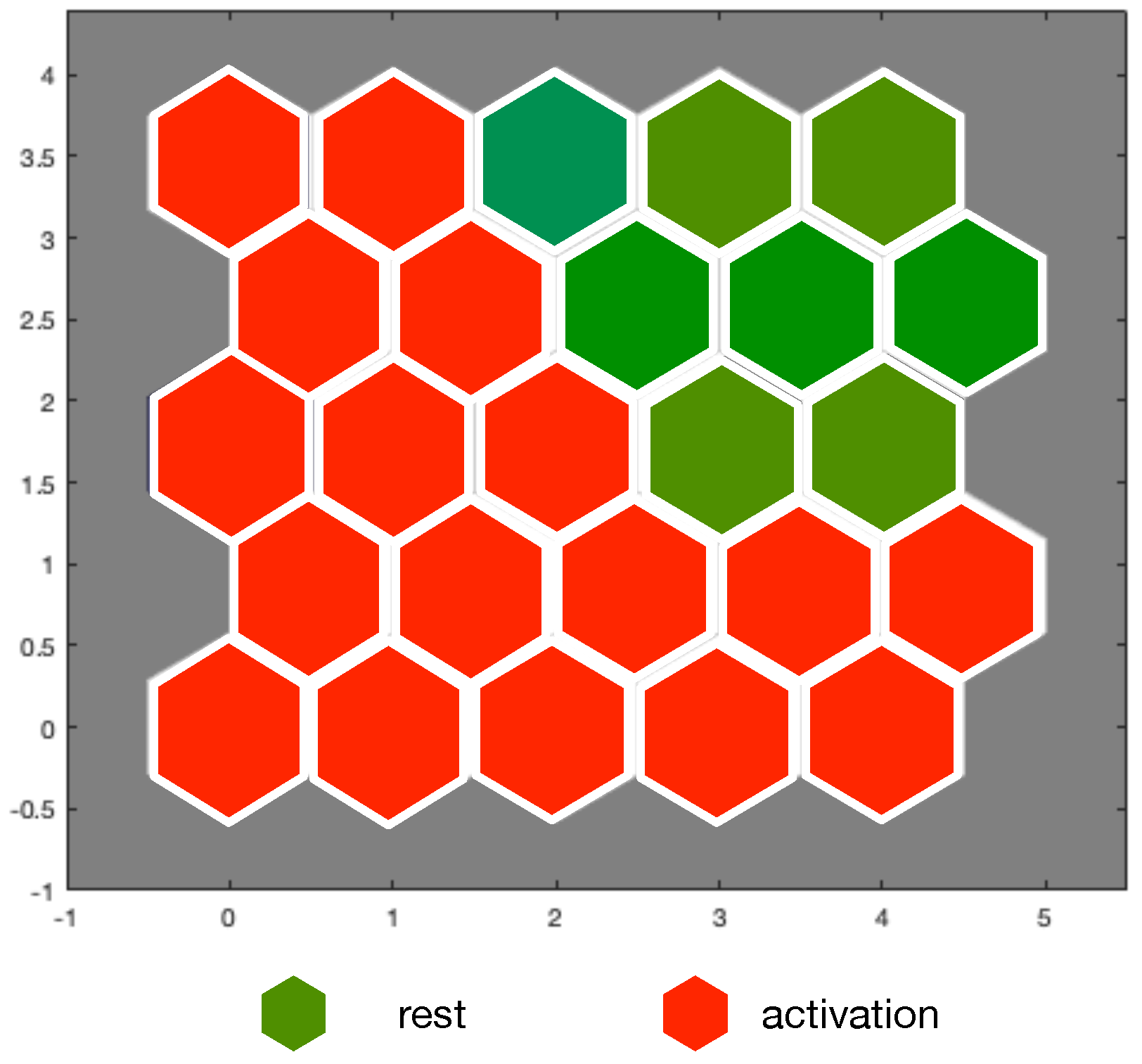
Map units can be a posteriori labeled according to several criteria. For example, using the majority-voting scheme as in [
46], we obtain the label map in
Figure 9. Comparing MCA hits maps with labels we obtain 3 misclassifications (2 false rests and one false activation). It is worth noting that misclassified patterns are next to units that would correctly classify them. It stands to reason that using larger maps trained on extended data could improve labeling result. On the other hand, majority-voting labeling can be sub-optimal and the use of fuzzy labeling [
47] should be preferred.
To summarize, results support that SOM has learned a topographic representation of the input space congruous with a priori data labels.
7. Discussion and Conclusions
In this work we reported on the use of a measurement setup aiming to the unobtrusive monitoring of psychophysical signals for detecting and analyzing potential stressing conditions in everyday life settings.
We have jointly analyzed two different datasets (MCA collected by our research group and SRAD from MIT Media lab). Aiming to assess stress activation, both were produced by recording a set of physiological signals in different settings. Our investigation was mainly conducted using the SRAD dataset (the most numerous) as development set, while MCA data were used for independent testing.
The work is focused on two main aspects: (a) recognition of activation statuses from resting ones and (b) building a comprehensive but compact description of individual status that could be useful in monitoring individual well-being.
From the original data space we extracted a set of 12 features including descriptors of HR, HRV, RR and GSR which are sensitive to individual response to stressors with emphasis on ANS response. Analysis of SRAD feature space by SFFS supports the conclusion that median RR and GSR peaks number has a prominent discriminating power and can lead to recognize activation statuses, which is also confirmed by MCA data analysis.
We also tested AE features obtained from the SRAD dataset. They are estimated using whole original data and are expected to reduce the potential information loss of SFFS mechanism. Results suggest that using two AE features can lead to good discrimination of rest states from activation ones. A similar conclusion is obtained using the same AE features for MCA dataset. It stands to reason that our data space is intrinsically two-dimensional with respect recognition of activation condition. This conclusion is also in accord with SFFS results.
Though the obtained results are consistent with background literature, they are in a sense surprising as the two datasets used for development and testing were acquired under completely different experimental conditions (while driving or while performing the SCWT). This supports the idea that the used feature set is highly descriptive of individual activation status and able to predict a wide spectrum of activation conditions. When applying standard k-means algorithm using the two most relevant features we observed two clusters that well represent rest and activation labels. This clustering is consistent with MCA data.
It must be pointed out that individual responses are intrinsically variable and the use of flexible but compact representations of individual status are highly desirable. In this context, the use of SOM networks revealed promising.
Being non-supervised, SOM can autonomously discover significant pieces of information embedded in data space. In addition, they project input data manifold onto network space by preserving topology and related structural properties such as clustering.
SOMs derived on SRAD data show the existence of two virtually separated zones in the map: one of them tends to respond to rest statuses, while the other best matches activation statuses. After labeling the SOM with a majority-voting scheme, we correctly classified 85% of MCA data blocks, as compared to 90% by k-means clustering with SFFS. SOM activation maps show that misclassification occurred next the border between the two groups. It is expected that using fuzzy labeling schemes along with extended training and testing data can lead to performance improvement.
A significant aspect of SOMs that is relevant for applications is their ability to discover and represent the internal structure of large clusters. In particular, each map unit can be viewed as a prototype (or code) of the individual’s status. In this view, activation (or rest) of a person is naturally represented by a structured family of codes. Investigation of the structure of such codes is our current focus of research. It will drive the acquisition of novel data and implementation of alternative SOM labeling.


