Predicting the Compressive Strength of Concrete Using an RBF-ANN Model

Abstract

In this study, a radial basis function (RBF) artificial neural network (ANN) model for predicting the 28-day compressive strength of concrete is established. The database used in this study is the expansion by adding data from other works to the one used in the author’s previous work. The stochastic gradient approach presented in the textbook is employed for determining the centers of RBFs and their shape parameters. With an extremely large number of training iterations and just a few RBFs in the ANN, all the RBF-ANNs have converged to the solutions of global minimum error. So, the only consideration of whether the ANN can work in practical uses is just the issue of over-fitting. The ANN with only three RBFs is finally chosen. The results of verification imply that the present RBF-ANN model outperforms the BP-ANN model in the author’s previous work. The centers of the RBFs, their shape parameters, their weights, and the threshold are all listed in this article. With these numbers and using the formulae expressed in this article, anyone can predict the 28-day compressive strength of concrete according to the concrete mix proportioning on his/her own.

1. Introduction

Concrete has characteristics of durability, impermeability, fire resistance, abrasion resistance, and high compressive strength. It can be cast into any shape and size. So, it is the most used construction material in the modern world. Its basic ingredients are water, cement, gravel which indicates the coarse aggregate, and sand which indicates the fine aggregate. For some environmental and sustainable considerations, various types of by-product materials are widely used as admixtures in concrete. The most commonly seen are the fly ash and the blast furnace slag. Some may also add other materials such as waste plastic, waste glass, rice husk, etc. [1,2,3,4,5,6]. Chemical and mineral admixtures might be added to enhance its workability or to change the time interval of the hardened state. The compressive strength is related to the proportioning of its ingredients. For economic reasons such as reducing the construction cost or saving the trial time for the strength requirement, the prediction of the compressive strength according to the proportioning design is a very important research topic. Studies have been implemented with mathematical models [7,8,9,10,11,12].

In recent decades, a lot of attention has been paid to the application of artificial neural networks (ANNs) in determining the compressive strength of concrete [13,14,15,16,17,18,19,20,21,22,23,24,25,26,27]. An ANN is like a black box. No theoretical relations between the compressive strength of concrete and the proportioning of its ingredients are needed for establishing an ANN model. The only requirement is the sufficiency of data for training and testing processes. With a well-trained ANN, one can input several numerical values which represent the proportioning of the concrete ingredients such as water, cement, sand, and other admixtures, and the ANN rapidly prompts out the predicted compressive strength of the concrete.

Typically, the database for the application of an ANN has to be divided into two sets, one for training and the other for testing. Usually, the testing set should contain more than 10 % of the database. Otherwise, the ANN has a tendency to over-fit the training set and will perform poorly in practical uses. In [27], an ANN model for predicting the 28-day compressive strength of concrete was established. They used the database of [26] in which an ANN model for the same application was also established. It was presumed that in [26] too little data were used for testing so that the ANN model was barely acceptable in the final validation. In [27], the data were rearranged. Fewer data were for training while more were used for testing. Therefore, the ANN model in [27] outperforms the one in [26], and it only has half the number of neurons in the hidden layer.

Both the ANN models in [26,27] are the back-propagation (BP) networks. Besides over-fitting, how to avoid over-training is another important issue when employing the BP-ANN. The ANN usually fits the training set better and better as more and more iterations of training are processed. However, it does not guarantee the over-trained ANN will also perform as well in practical uses. Because the training procedure of BP-ANN is extremely time-consuming, it is difficult to determine how many iterations of training are too excessive. In addition, it sometimes converges to a state of local minimum error.

Apart from the BP-ANN, there are many other types of ANNs. One of them is the Radial Basis Function (RBF) network. Unlike the BP-ANN, the solution of RBF-ANN is obtained in a rather straightforward way. The RBF centers and their shape parameters are usually determined in advance, then the weights are determined by the least-squares approach for a linear algebraic system in which the solution is unique. The only concern is how to choose the RBF centers and their shape parameters properly. Some may use the k-means approach to set the cluster centers as the RBF centers. Recently, other advanced algorithms have been employed in determining the RBF centers and their shape parameters in the RBF-ANNs which are widely used in various research areas [28,29,30,31,32,33,34].

In this paper, an RBF-ANN model for predicting the 28-day compressive strength of concrete is established. The database in [26] which was also used by [27] for establishing their model is expanded by adding more data listed in [35,36,37,38,39]. The Stochastic Gradient Approach presented in [40] is employed for determining the centers of RBFs and their shape parameters. Further validations are implemented by using the data of [25,26]. The results are compared with actual values as well as with the results of [27].

2. The Concrete Mix Proportioning

According to [26], the 28-day compressive strength of concrete is mainly related to seven factors. They are the mass of water, cement, fine aggregate (sand), coarse aggregate (gravel), blast furnace slag, fly ash, and superplasticizer mixed in 1 m³ concrete. Therefore, the 28-day compressive strength of concrete can be expressed as a mathematical function with seven arguments:

$$y=f(x)$$

(1)

in which

$$x={\left[\begin{array}{cccc}{x}_1& x_2& \cdots & x_7\end{array}\right]}^T$$

(2)

where $x_1$ to $x_7$ are the abovementioned proportioning factors while $y$ is the 28-day compressive strength of concrete. For the input and output of the ANN, all the data have to be normalized into the same range. In this paper, the raw data are transformed into the range of 0 to 1 linearly.

$${\xi }_i=\frac{x_i-x_{i,}{}_{\min }}{x_{i,}{}_{\max }-x_{i,}{}_{\min }}$$

(3)

$$\eta =\frac{y-y_{\min }}{y_{\max }-y_{\min }}$$

(4)

The database in [26] which was also used by [27] for establishing their model is expanded by adding 89 pieces of data listed in [35,36,37,38,39]. Totally, there are 571 data in the database. The testing set is the same as in [27], so 72 pieces of data are for testing while 499 pieces of data are for training. The size of the testing set is about 12.6% of the database. Printing out all the data might make this paper redundant. Those who need the raw data may find them in the references [26,27,35,36,37,38,39]. The ranges from $x_1$ to $x_7$ and $y$ are listed in

Table 1. The ranges of the inputs and the output of the raw data [26,27,35,36,37,38,39].

	Factors	Symbol	Maximum	Minimum	Unit
Inputs	water	x1	295	116.5	kg/m3
	cement	x2	643	74	kg/m3
	fine aggregate (sand)	x3	1293	30	kg/m3
	coarse aggregate (gravel)	x4	1226	436	kg/m3
	blast furnace slag	x5	440	0	kg/m3
	fly ash	x6	330	0	kg/m3
	superplasticizer	x7	27.17	0	kg/m3
Output	28-day compressive strength	y	95.3	5	MPa

. It is worthy to note that some of the values listed in Table 1 are slightly different from those in [27]. This is because the database has been expanded by adding data from other literature.

3. The RBF Artificial Neural Network

Now we have the function $\varphi$ with 7 arguments:

$$\eta =\varphi (\mathbf{\xi })$$

(5)

in which

$$\xi ={\left[\begin{array}{cccc}{\xi }_1& {\xi }_2& \cdots & {\xi }_7\end{array}\right]}^T$$

(6)

where all the arguments are in the range of 0 to 1. The linear combination of n RBFs is applied to approximate the input-output relation:

$$\eta \approx \widehat{\eta }=w_0+{\displaystyle \sum _{j=1}^n{w}_j{g}_j}(\mathbf{\xi })$$

(7)

in which $g_j$ is the j-th RBF and $w_j$ is its weight while $w_0$ represents the threshold. The larger value of n indicates the better the RBF-ANN fits the input-output relation in the training data, but it also has a higher risk of over-fitting. With N pieces of training data, i.e., N sets of ${\xi }_1$, ${\xi }_2$, …, ${\xi }_7$ and $\eta$, a linear-algebraic system can be formed

$$AW=\mathbf{\eta }$$

(8)

in which

$$A=\left[\begin{array}{cccccc}1& g_1\left({\xi }_1\right)& \cdots & \cdots & \cdots & g_n\left({\xi }_1\right)\\ 1& ⋮& \ddots & & & ⋮\\ ⋮& ⋮& & g_j\left({\xi }_i\right)& & ⋮\\ ⋮& ⋮& & & \ddots & ⋮\\ 1& g_1\left({\xi }_N\right)& \cdots & \cdots & \cdots & g_n\left({\xi }_N\right)\end{array}\right]$$

(9)

$$W={\left[\begin{array}{cccccc}{w}_0& w_1& \cdots & w_j& \cdots & w_n\end{array}\right]}^T$$

(10)

$$\eta ={\left[\begin{array}{cccccc}{\eta }_1& {\eta }_2& \cdots & {\eta }_i& \cdots & {\eta }_N\end{array}\right]}^T$$

(11)

where ${\xi }_i$ and ${\eta }_i$ represent the input and output of the i-th piece of data. Equation (8) is a combination of N linear equations subjected with n + 1 unknowns which are the threshold $w_0$ and the weights $w_1$, $w_2$, …, $w_n$. The least-square-error solution can be obtained promptly by using the following matrix operation.

$$W={\left(A^{T}A\right)}^{-1}{A}^T\eta$$

(12)

Among many RBFs, the Gaussian RBF is chosen in this study:

$$g_j\left(\xi \right)=\exp \left(-{\Vert \xi -{\zeta }_j\Vert }^2/{\sigma }_j^2\right)$$

(13)

in which ${\zeta }_j$ represents the center of the jth RBF

$${\zeta }_j={\left[\begin{array}{cccc}{\zeta }_{j1}& {\zeta }_{j2}& \cdots & {\zeta }_{j7}\end{array}\right]}^T$$

(14)

while ${\sigma }_j$ is the shape parameter and $\Vert \xi -{\zeta }_j\Vert$ denotes the Euclidean distance from $\xi$ to ${\zeta }_j$. Ususally, the centers of RBFs and their shape parameters are manually pre-determined. Some may use the k-means approach to set n cluster centers as the RBF centers. Recently, advanced algorithms like tabu and genetic are employed to determine them [30,32,34]. The structure of this RBF-ANN is similar to the one-hidden-layer BP-ANN which has just one output. An RBF can be deemed as a neuron in the hidden layer. The RBF centers are analogous to the synaptic weights from the input layer to the hidden layer. The shape parameters of the RBFs are similar to the biases (or thresholds) of the hidden neurons. The weights of the RBFs are like the connections from the hidden layer to the output while the threshold in Equation (7) is similar to the bias (or the threshold) of the output neuron in the BP-ANN.

4. The Algorithm for Determining the Centers of RBFs and Their Shape Parameters

Though there are some advanced algorithms for determining the centers of RBFs and their shape parameters, the stochastic gradient approach presented in the textbook [40] is employed in this study. It was found in [27] that a single-hidden-layer ANN which composes just a few neurons in the hidden layer is sufficient for this application. Therefore, using the stochastic gradient approach is presumed to be enough. Besides, in the author’s previous work [41] which was about solving the partial differential equations with the RBFs, the advantages of the stochastic gradient approach were clearly demonstrated.

Initially, all the values of ${\sigma }_j$ and ${\zeta }_{jk}$, in which $j=1~n$ and $k=1~7$, are randomly chosen. For the reason that a negative $\sigma$ is meaningless and too large $\sigma$ makes the Gaussian RBF behave like a constant, ${\sigma }_j$ is confined just in the range of 0 to 10. Similarly, a too far Euclidean distance from $\xi$ to ${\zeta }_j$ is also meaningless, so all the components of ${\zeta }_j$ are confined in the range from −1 to 2, for the reason that all the components of $\xi$ are just in the range of 0 to 1. After using Equation (12) to obtain the threshold $w_0$ and the weights $w_1$, …, $w_n$, the error $e_i$ corresponding to the ith piece of data can be calculated

$$e_i={\widehat{\eta }}_i-{\eta }_i$$

(15)

in which ${\eta }_i$ is the exact output while ${\widehat{\eta }}_i$ is the predicted output by the RBF-ANN. The total square error is summed up as

$$E={\displaystyle \sum _{i=1}^N{e}_i^2}$$

(16)

The value of $E$ is now dependant on values of ${\sigma }_j$ and ${\zeta }_{jk}$. We can use the following formulae to update their values:

$${\sigma }_j^{(\mathrm{new})}={\sigma }_j^{(\mathrm{old})}-\mu \frac{\partial E}{\partial {\sigma }_j}$$

(17)

$${\zeta }_{jk}^{(\mathrm{new})}={\zeta }_{jk}^{(\mathrm{old})}-\mu \frac{\partial E}{\partial {\zeta }_{jk}}$$

(18)

in which $\mu$ is called the stepping parameter. Smaller $\mu$ results in a steady convergence but might make it trapped in a state of local minimum error. On the other hand, larger $\mu$ results in instability but may help to escape from the strap. In this study, $\mu$ is set as a relaxation coefficient that varies according to the situation of convergence.

$$\mu =\{\begin{array}{ll}1000{\mu }^{(p)}\hfill & , \mathrm{if} {\mu }^{(p)}<0.01{\mu }^{(i)}\hfill \\ 10{\mu }^{(p)}\hfill & , \mathrm{else} \mathrm{if} N_{iter}/200=Int(N_{iter}/200)\hfill \\ 1.03{\mu }^{(p)}\hfill & , \mathrm{else} \mathrm{if} E<E^{(p)}\hfill \\ 0.5{\mu }^{(p)}\hfill & , \mathrm{otherwise}\hfill \end{array}$$

(19)

in which the superscript (p) denotes the word “previous” and the superscript (i) denotes the word “initial”, $N_{iter}$ represents the number of processed iterations, and the operator “Int(●)” means taking the integer part of a floating number. Multiplying $\mu$ by 1000 or by 10 can help to escape from the state of local minimum error. The initial value of $\mu$ is 0.01. The training algorithm is listed as follows.

• Step 1: Randomly set initial values for ${\sigma }_j$ and ${\zeta }_{jk}$. ($j=1~n$ and $k=1~7$)
• Step 2: Use Equation (12) to obtain the threshold $w_0$ and the weights $w_j$.
• Step 3: Calculate the error $e_i$ for each piece of the training data ($i=1~N$), then sum up the total square error $E$.
• Step 4: If the total square error $E$ is the smallest so far, save the values of $w_0$, $w_j$, ${\sigma }_j$ and ${\zeta }_{jk}$ in a file.
• Step 5: If the smallest $E$ has not been updated for 500,000 times of training iteration, reset ${\sigma }_j$ and ${\zeta }_{jk}$ with random values and go back to Step 2.
• Step 6: Use Equation (19) to set the stepping parameter $\mu$.
• Step 7: Update all the values of ${\sigma }_j$ and ${\zeta }_{jk}$ by using Equations (17) and (18).
• Step 8: Repeat Steps 2 to 7 and stop when the required number of iterations is achieved.

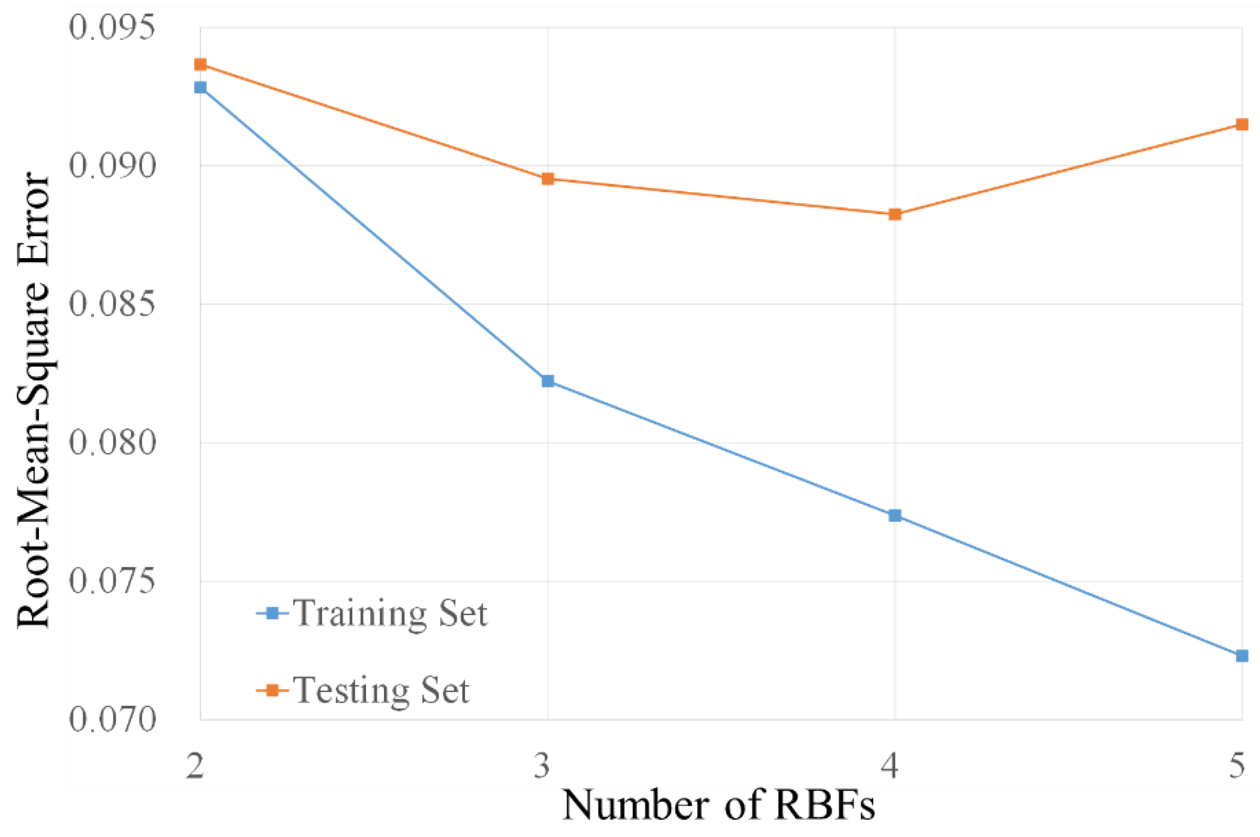
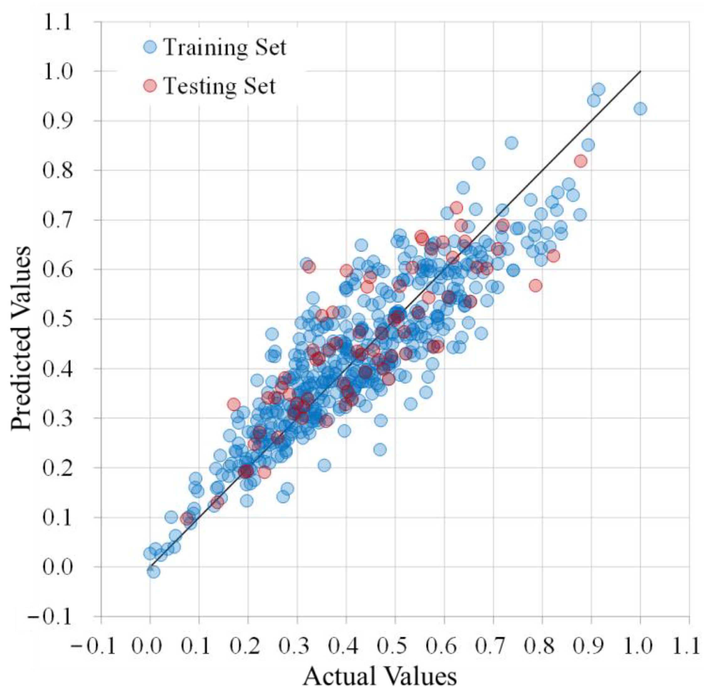
5. The Results of Training and Testing

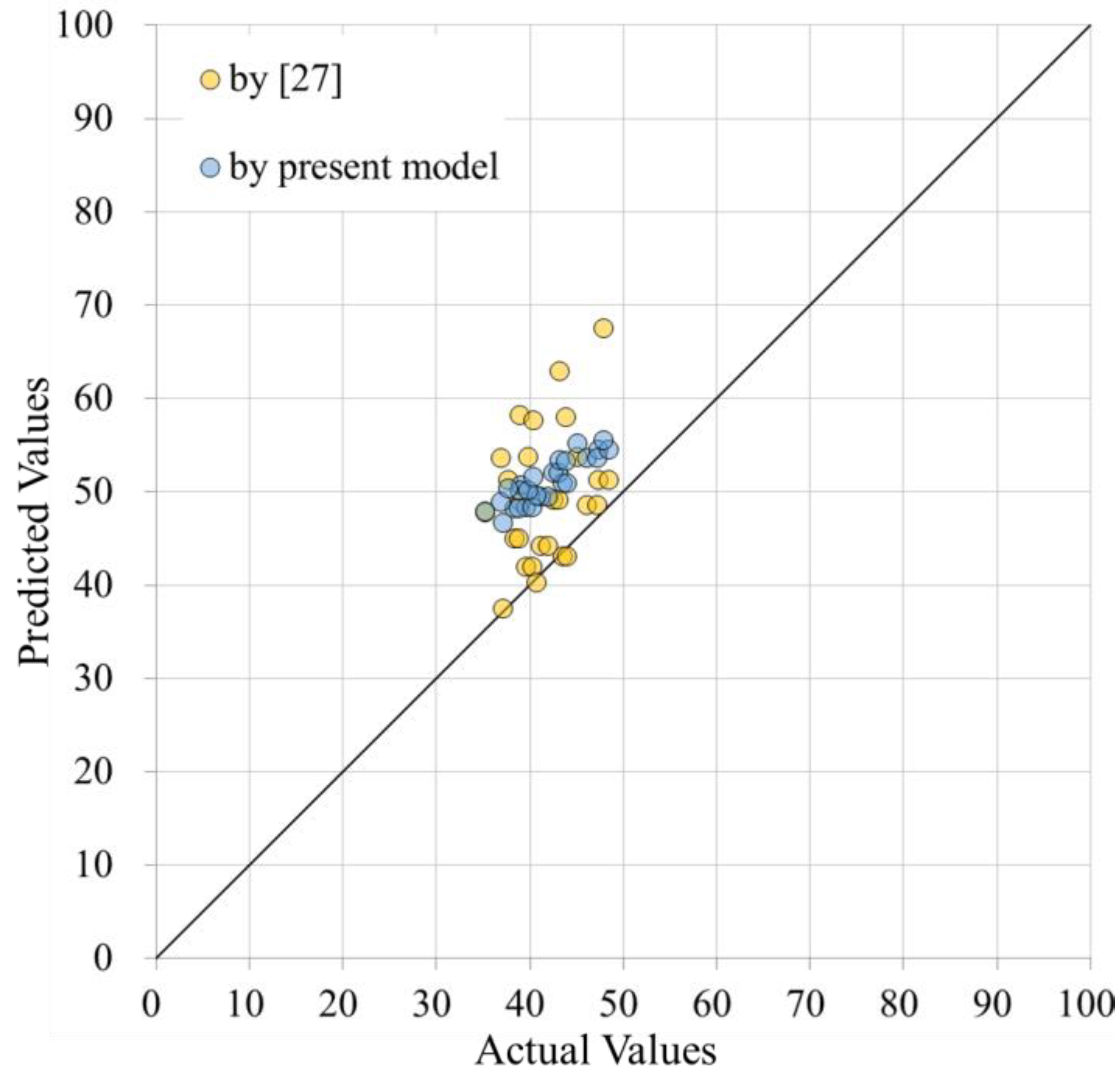
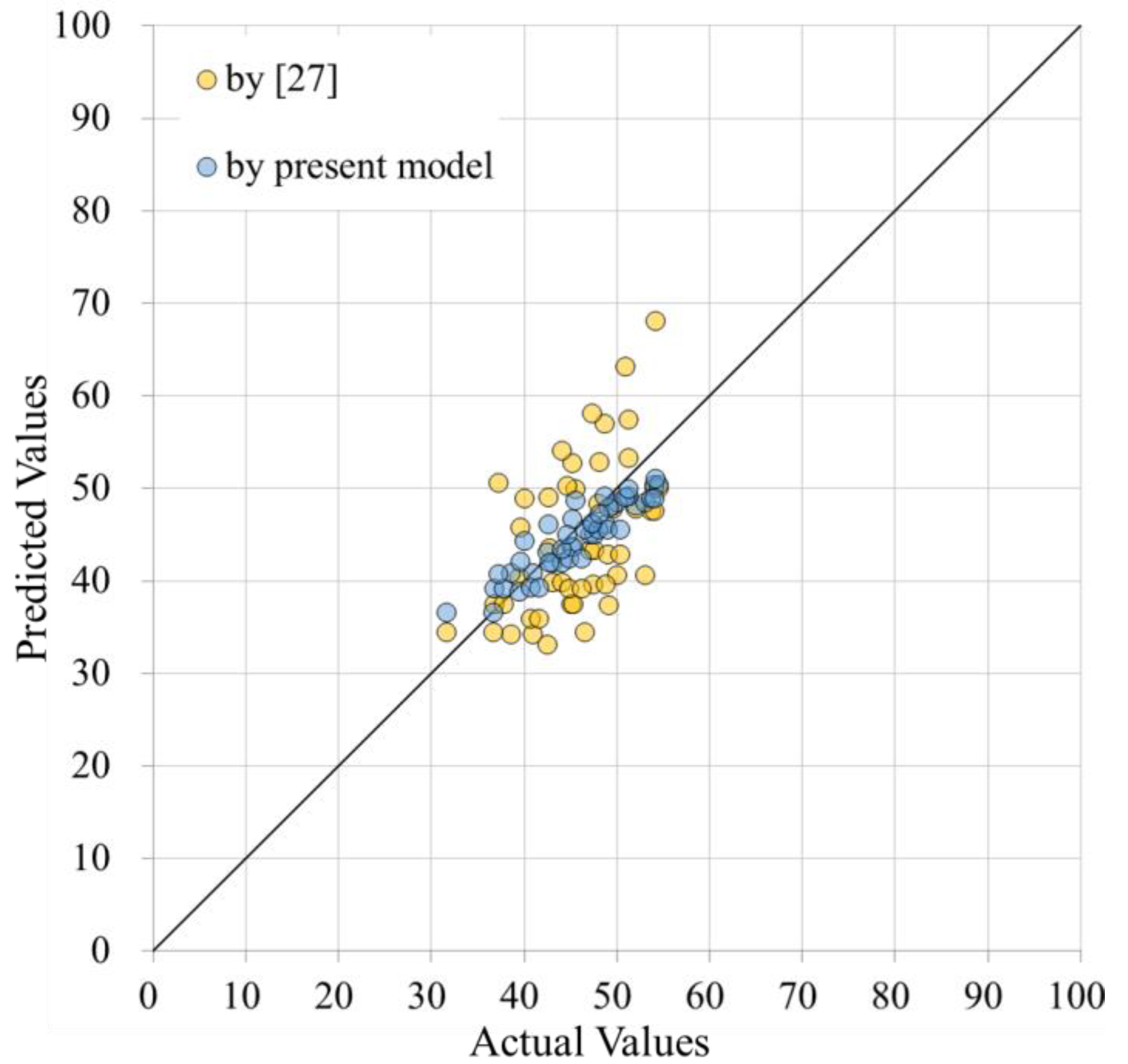
The computer program is coded with Fortran 90 and compiled with the X64 compiler of Intel^®-Fortran 2016. Each run uses only one processor of the computer of Intel^® Core™ i7-8700CPU @3.20GHz 3.19GHz. Artificial neural networks with 2–5 RBFs are trained and tested. Each RBF-ANN is trained with three runs in which $2\times {10}^8$ iterations are processed. The computational time does not increase linearly with the number of RBFs. For the ANNs with 2 RBFs, the computational time is 2.98 h. As per those with 3, 4, and 5 RBFs, the computational times are 4.25, 5.56, and 6.81 h respectively. Though the centers of RBFs and their shape parameters are all set up with random numbers, after $2\times {10}^8$ iterations of training, the ANNs with the same number of RBFs converge to results that are very close to each other. That means the convergence is valid for sure. It also confirms the presumption that using the stochastic gradient approach is enough. For the ANNs with just 2 or 3 RBFs, converging to the final result just needs several million times of iteration, which means the convergence is achieved within 1 hour.

The root-mean-square error is employed to examine the performance of the trained ANNs.

$$E_{r.m.s.}=\sqrt{ \overline{{\left(\eta -\widehat{\eta }\right)}^2}}$$

(20)

where the overbar represents the average in the data set. Note that the numbers of data in the training set and testing set are 499 and 72, respectively. The results of training and testing are plotted in Figure 1.

It is found that setting more RBFs in the ANN results in smaller $E_{r.m.s.}$ in the training set. However, it does not go the same way in the testing set. This implies too many RBFs in the ANN have a risk of over-fitting. Though the ANN with 4 RBFs fits testing data the best, using just 3 RBFs is supposed to be safer from over-fitting. The comparisons of exact values and the predicted values by the ANN with 3 RBFs are shown in Figure 2. Note that the plotted values in this figure are the normalized values. The root-mean-square errors of the training set and the testing set are 0.0822 and 0.0895, respectively. It is worthy to note that the testing set is the same as in [27] while the RBF-ANN in this study fits the testing set better. The root-mean-square error of the testing set in [27] was 0.0914.

Finally, the centers of the 3 RBFs are listed here.

$${\zeta }_1={\left[\begin{array}{rrrrrrr}\hfill -1.00000& \hfill -1.00000& \hfill 0.44034& \hfill 0.60326& \hfill -0.00486& \hfill 0.52630& \hfill 1.24615\end{array}\right]}^T$$

(21)

$${\zeta }_2={\left[\begin{array}{rrrrrrr}\hfill -0.84767& \hfill 0.61160& \hfill 0.46294& \hfill 0.56556& \hfill 0.67973& \hfill 0.61628& \hfill 0.65405\end{array}\right]}^T$$

(22)

$${\zeta }_3={\left[\begin{array}{rrrrrrr}\hfill -0.55917& \hfill 1.05027& \hfill 1.08523& \hfill 0.79403& \hfill 0.86121& \hfill 0.77691& \hfill 0.46370\end{array}\right]}^T$$

(23)

The shape parameters of these 3 RBFs are 2.06819, 0.90677, and 0.45945, respectively. Their weights are −4.17952, 11.2345, and −5275.82 while the threshold is 1.05900. With these numbers, one can use Equations (7) and (13) to calculate the corresponding output of the ANN by any input. The 28-day compressive strength of the concrete can be retrieved by using the backward transform of Equation (4).

6. The Verification

Additional 12 mix designs listed in [26] are used for the verification of the present RBF-ANN model. They are excluded from the database for training and testing. The predicted values are also compared with those predicted by the BP-ANN models in [26,27]. The results are plotted in Figure 3. It should be noted that the values plotted in this figure are the values of the 28-day compressive strength of concrete whose range in the database is from 5 MPa to 95.3 MPa. The $E_{r.m.s.}$ by using the present RBF-ANN model is 7.53 MPa. It performs a little worse than the BP-ANN model in [27] whose $E_{r.m.s.}$ is just 4.73 MPa. As per the comparison with the BP-ANN model in [26] whose $E_{r.m.s.}$ is 10.70 MPa, the present RBF-ANN is still better.

In [25], the genetic algorithm was employed to train the artificial neural network which was established to predict the 28-day, 56-day, and 91-day compressive strengths of concrete admixing with fly ash or without fly ash. Blast furnace slag and superplasticizer are not admixed in their samples. Though the predicted results of [25] were not listed in their paper, the actual compressive strengths were available. So, the data were used to validate the BP-ANN model of [27] further. Here, the data in [25] are also used to validate the present RBF-ANN model. The comparisons of the predicted and the actual 28-day compressive strengths of the concrete admixed with and without fly ash are plotted in Figure 4 and Figure 5. For those admixed with fly ash, the present RBF-ANN model has a root-mean-square error of 9.42 MPa while the BP-ANN model of [27] performs with the root-mean-square error of 10.28 MPa. Both ANN models over-estimate the compressive strength, but the results of the present model are generally closer to the actual values. For those admixed without fly ash, the root-mean-square errors are 2.65 MPa and 7.19 MPa, respectively. The present model performs much better than the model in [27].

The result is quite reasonable because the variation of particle sizes and the chemical composition in different fly ash may be the source of some uncertainties. Generally speaking, the performance of the present RBF-ANN is quite acceptable.

7. Conclusions

The focus of this study is on establishing an RBF-ANN model for predicting the 28-day concrete compressive strength according to the proportioning of the ingredients. The stochastic gradient approach present in [40] is employed for tuning the centers of RBFs and their shape parameters. Using a similar treatment in [41], the stepping parameter in the stochastic gradient approach is treated as a relaxation coefficient which can help to escape from the solution of local minimum error. An RBF in the ANN is analogous to a neuron in the BP-ANN which was employed for the same purpose in the author’s previ-ous work [27]. Artificial neural networks with 2–5 RBFs are trained and tested. Each RBF-ANN is trained with 3 runs in which $2\times {10}^8$ iterations are processed. After the iteration processes, all the ANNs with the same number of RBFs converge to results that are very close to each other. This implies the convergence is valid. Therefore, the only issue concerning over-fitting is the number of RBFs. Finally, the ANN with just 3 RBFs is chosen for further verification. Data for verification are the same as those used in the author’s previous work [27] so they can be compared. The comparisons show that the present model performs better than the author’s previous model [27] which was established by using the BP-ANN and has 7 neurons in the hidden layer.

The centers of the RBFs, their shape parameters, their weights, and the threshold are all listed in this article. With these numbers and using Equations (3), (4), (7) and (13), anyone can predict the compressive strength of concrete according to the concrete mix proportioning on his/her own.

References

1. Al-Manaseer, A.A.; Dalal, T.R. Concrete containing plastic aggregates. Concr. Int. 1997, 19, 47–52. [Google Scholar]
2. Jin, W.; Meyer, C.; Baxter, S. Glasscrete—Concrete with glass aggregate. ACI Mater. J. 2000, 97, 208–213. [Google Scholar]
3. Coutinho, J.S. The combined benefits of CPF and RHA in improving the durability of concrete structures. Cem. Concr. Compos. 2003, 25, 51–59. [Google Scholar] [CrossRef]
4. Batayneh, M.; Marie, I.; Asi, I. Use of selected waste materials in concrete mixes. Waste Manag. 2007, 27, 1870–1876. [Google Scholar] [CrossRef]
5. Siddique, R. Waste Materials and By-Products in Concrete; Springer: Berlin/Heidelberg, Germany, 2008. [Google Scholar]
6. Paul, S.C.; Panda, B.; Garg, A. A novel approach in modelling of concrete made with recycled aggregates. Measurement 2018, 115, 64–72. [Google Scholar] [CrossRef]
7. Tsivilis, S.; Parissakis, G. A mathematical-model for the prediction of cement strength. Cem. Concr. Res. 1995, 25, 9–14. [Google Scholar] [CrossRef]
8. Kheder, G.F.; Al-Gabban, A.M.; Abid, S.M. Mathematical model for the prediction of cement compressive strength at the ages of 7 and 28 days within 24 hours. Mater. Struct. 2003, 36, 693–701. [Google Scholar] [CrossRef]
9. Akkurt, S.; Tayfur, G.; Can, S. Fuzzy logic model for the prediction of cement compressive strength. Cem. Concr. Res. 2004, 34, 1429–1433. [Google Scholar] [CrossRef] [Green Version]
10. Hwang, K.; Noguchi, T.; Tomosawa, F. Prediction model compressive strength development of fly-ash concrete. Cem. Concr. Res. 2004, 34, 2269–2276. [Google Scholar] [CrossRef]
11. Zelić, J.; Rušić, D.; Krstulović, R. A mathematical model for prediction of compressive strength in cement-silica fume blends. Cem. Concr. Res. 2004, 34, 2319–2328. [Google Scholar] [CrossRef]
12. Zain, M.F.M.; Abd, S.M. Multiple regressions model for compressive strength prediction of high performance concrete. J. Appl. Sci. 2009, 9, 155–160. [Google Scholar] [CrossRef]
13. Ni, H.-G.; Wang, J.-Z. Prediction of compressive strength of concrete by neural networks. Cem. Concr. Res. 2000, 30, 1245–1250. [Google Scholar] [CrossRef]
14. Lee, S.-C. Prediction of concrete strength using artificial neural networks. Eng. Struct. 2003, 25, 849–857. [Google Scholar] [CrossRef]
15. Öztaş, A.; Pala, M.; Özbay, E.; Kanca, E.; Çaĝlar, N.; Bhatti, M.A. Predicting the compressive strength and slump of high strength concrete using neural network. Constr. Build. Mater. 2006, 20, 769–775. [Google Scholar] [CrossRef]
16. Topçu, I.B.; Sarıdemir, M. Prediction of compressive strength of concrete containing fly ash using artificial neural networks and fuzzy logic. Comput. Mater. Sci. 2008, 41, 305–311. [Google Scholar] [CrossRef]
17. Alshihri, M.M.; Azmy, A.M.; El-Bisy, M.S. Neural networks for predicting compressive strength of structural light weight concrete. Constr. Build. Mater. 2009, 23, 2214–2219. [Google Scholar] [CrossRef]
18. Bilim, C.; Atiş, C.D.; Tanyildizi, H.; Karahan, O. Predicting the compressive strength of ground granulated blast furnace slag concrete using artificial neural network. Adv. Eng. Softw. 2009, 40, 334–340. [Google Scholar] [CrossRef]
19. Sobhani, J.; Najimi, M.; Pourkhorshidi, A.R.; Parhizkar, T. Prediction of the compressive strength of no-slump concrete: A comparative study of regression, neural network and ANFIS models. Constr. Build. Mater. 2010, 24, 709–718. [Google Scholar] [CrossRef]
20. Atici, U. Prediction of the strength of mineral admixture concrete using multivariable regression analysis and an artificial neural network. Expert Syst. Appl. 2011, 38, 9609–9618. [Google Scholar] [CrossRef]
21. Chou, J.-S.; Chiu, C.-K.; Farfoura, M.; Al-Taharwa, I. Optimizing the prediction accuracy of concrete compressive strength based on a comparison of data-mining techniques. J. Comput. Civ. Eng. 2011, 25, 242–253. [Google Scholar] [CrossRef]
22. Duan, Z.H.; Kou, S.C.; Poon, C.S. Prediction of compressive strength of recycled aggregate concrete using artificial neural networks. Constr. Build. Mater. 2013, 40, 1200–1206. [Google Scholar] [CrossRef]
23. Chopra, P.; Sharma, R.K.; Kumar, M. Artificial Neural Networks for the Prediction of Compressive Strength of Concrete. Int. J. Appl. Sci. Eng. 2015, 13, 187–204. [Google Scholar]
24. Nikoo, M.; Moghadam, F.T.; Sadowski, L. Prediction of Concrete Compressive Strength by Evolutionary Artificial Neural Networks. Adv. Mater. Sci. Eng. 2015, 2015, 849126. [Google Scholar] [CrossRef]
25. Chopar, P.; Sharma, R.K.; Kumar, M. Prediction of Compressive Strength of Concrete Using Artificial Neural Network and Genetic Programming. Adv. Mater. Sci. Eng. 2016, 2016, 7648467. [Google Scholar] [CrossRef] [Green Version]
26. Hao, C.-Y.; Shen, C.-H.; Jan, J.-C.; Hung, S.-K. A Computer-Aided Approach to Pozzolanic Concrete Mix Design. Adv. Civ. Eng. 2018, 2018, 4398017. [Google Scholar]
27. Lin, C.-J.; Wu, N.-J. An ANN Model for Predicting the Compressive Strength of Concrete. Appl. Sci. 2021, 11, 3798. [Google Scholar] [CrossRef]
28. Segal, R.; Kothari, M.L.; Madnani, S. Radial basis function (RBF) network adaptive power system stabilizer. IEEE Trans. Power Syst. 2000, 15, 722–727. [Google Scholar] [CrossRef]
29. Mai-Duy, N.; Tran-Cong, T. Numerical solution of differential equations using multiquadric radial basis function networks. Neural Netw. 2001, 14, 185–199. [Google Scholar] [CrossRef] [Green Version]
30. Ding, S.; Xu, L.; Su, C.; Jin, F. An optimizing method of RBF neural network based on genetic algorithm. Neural Comput. Appl. 2012, 21, 333–336. [Google Scholar] [CrossRef]
31. Li, Y.; Wang, X.; Sun, S.; Ma, X.; Lu, G. Forecasting short-term subway passenger flow under special events scenarios using multiscale radial basis function networks. Transp. Res. Part C Emerg. Technol. 2017, 77, 306–328. [Google Scholar] [CrossRef]
32. Aljarah, C.I.; Faris, H.; Mirjalili, S.; Al-Madi, N. Training radial basis function networks using biogeography-based optimizer. Neural Comput. Appl. 2018, 29, 529–553. [Google Scholar] [CrossRef]
33. Hong, H.; Zhang, Z.; Guo, A.; Shen, L.; Sun, H.; Liang, Y.; Wu, F.; Lin, H. Radial basis function artificial neural network (RBF ANN) as well as the hybrid method of RBF ANN and grey relational analysis able to well predict trihalomethanes levels in tap water. J. Hydrol. 2020, 591, 125574. [Google Scholar] [CrossRef]
34. Karamichailidou, D.; Kaloutsa, V.; Alexandridis, A. Wind turbine power curve modeling using radial basis function neural networks and tabu search. Renew. Energy 2021, 163, 2137–2152. [Google Scholar] [CrossRef]
35. Jiang, L.H.; Malhotra, V.M. Reduction in water demand of non-air-entrained concrete incorporating large volumes of fly ash. Cem. Concr. Res. 2000, 30, 1785–1789. [Google Scholar] [CrossRef]
36. Demirboğa, R.; Türkmen, İ.; Karakoç, M.B. Relationship between ultrasonic velocity and compressive strength for high-volume mineral-admixtured concrete. Cem. Concr. Res. 2004, 34, 2329–2336. [Google Scholar] [CrossRef]
37. Yen, T.; Hsu, T.-H.; Liu, Y.-W.; Chen, S.-H. Influence of class F fly ash on the abrasion–erosion resistance of high-strength concrete. Constr. Build. Mater. 2007, 21, 458–468. [Google Scholar] [CrossRef]
38. Oner, A.; Akyuz, S. An experimental study on optimum usage of GGBS for the compressive strength of concrete. Cem. Concr. Compos. 2007, 29, 505–514. [Google Scholar] [CrossRef]
39. Durán-Herrera, A.; Juárez, C.A.; Valdez, P.; Bentz, D.P. Evaluation of sustainable high-volume fly ash concretes. Cem. Concr. Compos. 2011, 33, 39–45. [Google Scholar] [CrossRef]
40. Ham, F.M.; Kostanic, I. Principles of Neurocomputing for Science & Engineering; McGraw-Hill Higher Education: New York, NY, USA, 2001. [Google Scholar]
41. Wu, N.-J.; Chang, K.-A. Simulation of free-surface waves in liquid sloshing using a domain-type meshless method. Int. J. Numer. Methods Fluids 2011, 67, 269–288. [Google Scholar] [CrossRef]
Figure 1. The performance of the trained radial basis functions-artificial neural networks (RBF-ANNs).
Applsci 11 06382 g001
Figure 2. The comparison of the outputs of ANN with their target values in which the ANN only has 3 RBFs.
Applsci 11 06382 g002
Figure 3. Comparison of the predicted values with the actual 28-day compressive strength of concrete [26] (Unit: MPa).
Applsci 11 06382 g003
Figure 4. Comparison of the predicted values with the actual 28-day compressive strength of concrete in which fly ash was admixed [25] (Unit: MPa).
Applsci 11 06382 g004
Figure 5. Comparison of the predicted values with the actual 28-day compressive strength of concrete in which no fly ash was admixed [25] (Unit: MPa).
Applsci 11 06382 g005