Credible Navigation Algorithm for GNSS Attack Detection Using Auxiliary Sensor System

Abstract

In order to effectively reduce the impact of Global Navigation Satellite System (GNSS) attacks while providing mobile terminals with credible navigation and positioning results, this paper proposes a credible navigation algorithm for GNSS attack detection using an auxiliary sensor system. Based on a credible Kalman filter and measurement information provided by the auxiliary sensor system on mobile terminals, the proposed algorithm can verify the credibility of the GNSS positioning result and determine whether it has suffered from a GNSS attack using the credible verification window and the credible verification threshold. According to the verification results, the algorithm can adaptively select an updated model for measurement correction and achieve a credible navigation result. The algorithm proposed in this paper has been verified on a self-developed mobile terminal, and the experimental results show that the algorithm can provide credible navigation and positioning services for mobile terminals in the context of GNSS attacks.

1. Introduction

The existing and widely used GNSS can provide all-day global Position, Navigation and Time (PNT) service. However, the GNSS signal is a type of radio signal and is vulnerable to attacks from other radio signals in the same frequency band. As a result, the GNSS signals acquired by mobile terminal often suffer from abnormalities, causing the deviation of filter parameters, which results in an incorrect movement trajectory received by the terminal and makes the navigation and positioning results undependable [1,2,3,4]. For autonomous driving and the Internet of Vehicles, the increase in the level of automation will also increase the chances of successful attacks by hackers, especially on the navigation control module based on the GNSS, which could substantially deteriorate the safety of the vehicle [5,6].

The main methods of GNSS signal attacks include suppressive interference and spoofing interference [7]. Suppressive interference uses high-power signal blocking to prevent the receiver from working normally, but it is relatively easy to be detected. On the other hand, spoofing interference works by transmitting signals that are the same as or similar to the real satellite signals in order to deceive the terminal which rely on navigation information for positioning, and this method is relatively difficult to detect. Therefore, spoofing interference has gradually become a bigger threat to satellite navigation systems. Spoofing interference upon the GNSS is usually conducted in three different forms: the auto-generating type, repeater type and inducing type [8]. Auto-generating spoofing utilizes public navigation signals to generate its own navigation signals autonomously and seize control of the receiver afterwards. This spoofing method is low in cost and simple to be implemented. However, the generated spoofing signal is far from the real signal and is easily detected. The repeater type of spoofing copies the received real signal, adds a delay, and forwards it again as a spoofing signal. This spoofing is mainly used for navigation signals whose interface files are not disclosed. However, in order to seize control, the power of the spoofing signal still needs to be further increased; moreover, this method also requires the interruption of the receiver to make it re-enter the capture state, which can be detected using the power detection method. Inducting spoofing is the only spoofing method that can seize control without changing the tracking state of the receiver. It is concealed and difficult to detect with conventional methods, such as power detection.

In order to improve the credibility of mobile terminal navigation and positioning, different detection technologies are used for different types of GNSS attacks [9,10,11]. Today, the detection technologies for GNSS attacks can be divided into the following categories [12]: signal encryption authentication, signal feature detection and consistency verification with other navigation sensors. The signal encryption authentication technology [13,14,15] is used to encrypt the civil navigation signal or spreading code to deal with spoofing interference. However, for the method to work, it is required to change the signal system, add a reference receiver, and rely on other networks for collaborative detection. Signal feature detection [16,17,18,19,20] detects spoofing based on the amplitude, arrival time and arrival angle during the GNSS receiver’s capture and tracking phase in order to determine the credibility of the GNSS signal. Compared to the previous one, this method does not need to change the signal system, but it requires upgrades to the baseband signal processing algorithm related to the GNSS receiver, or installation of anti-jamming modules, which are very expensive. The consistency verification of the mobile terminal combined with the auxiliary navigation sensors already installed on the mobile terminal can also effectively realize the detection of GNSS jamming and spoofing. Currently, the commonly seen mobile terminals that use GNSS signals, such as automobiles, aircraft, individual soldiers and unmanned terminals, are usually equipped with auxiliary navigation sensors [21] such as inertial measurement units (IMUs), odometers, etc. These auxiliary navigation sensors are non-radio sensors and will not be attacked by GNSS jamming signals or GNSS spoofing signals. These sensors can provide navigation and positioning information with good accuracy in a short time with high update rate. The position coordinates calculated by the auxiliary navigation sensors will be continuous, with no sudden interruption or signal jump.

By effectively using the measurement information provided by the auxiliary navigation sensors to check the consistency of the GNSS signal, the mobile terminal is capable of detecting the involving jamming and spoofing attacks. Reference [22] proposed an accelerometer-assisted spoofing detection algorithm, which compares the difference between accelerometer output and the GPS output to detect anomalies caused by spoofing interference. Reference [23] proposed a joint spatial consistency check method that judges whether the positioning solution meets the distance constraint to counter GNSS spoofing attacks according to the known position provided by the GNSS receiver. Reference [24] proposed a method that fuses the GNSS absolute positioning data with the data of the vehicle speed sensor, acceleration sensor, and steering wheel angle sensor so that it can still provide accurate vehicle positioning even when the GNSS signal is interrupted for a short period of time. Reference [25] proposed a method for predicting the position deviation of UAVs under GPS spoofing attacks based on innovative particle filters. The integrated architecture of GPS/Loran-C/INS improves the accuracy of UAV’s true position prediction. These methods mentioned above all use measurement navigation information provided by auxiliary navigation sensors for signal attacking detection without increasing the user’s hardware cost. However, when induced spoofing attacks occur, the calibration feedback information of the Kalman Filter system in these methods will be biased due to GNSS spoofing. Therefore, reference [26] proposed a MEMS-INS/GNSS tightly coupled spoofing identification method based on the estimation of the spoofing contour: it reconstructs and analyzes the spoofing distribution to predict GNSS attacks in the signal domain and effectively identifies and eliminates induced spoofing attacks.

In response to the problems discussed above, the purpose of this article is to design a simple and effective navigation algorithm to detect and mitigate different kinds of GNSS attacks, including GNSS jamming or GNSS spoofing, and then obtain a credible navigation result in the positioning domain. Therefore, a credible navigation algorithm for GNSS attacks detection using an auxiliary sensor system (ACNA) is proposed. By monitoring the measurement information of the GNSS and the auxiliary navigation sensors in the location domain during the credible verification window, the ACNA method analyzes and determines whether the mobile terminal suffers a GNSS attack. According to the verifications, the algorithm can adaptively select an updated model for measurement correction, and output credible navigation results. Finally, through the data sets collected by the self-developed mobile terminal, the analysis and verification of the algorithm performance are verified.

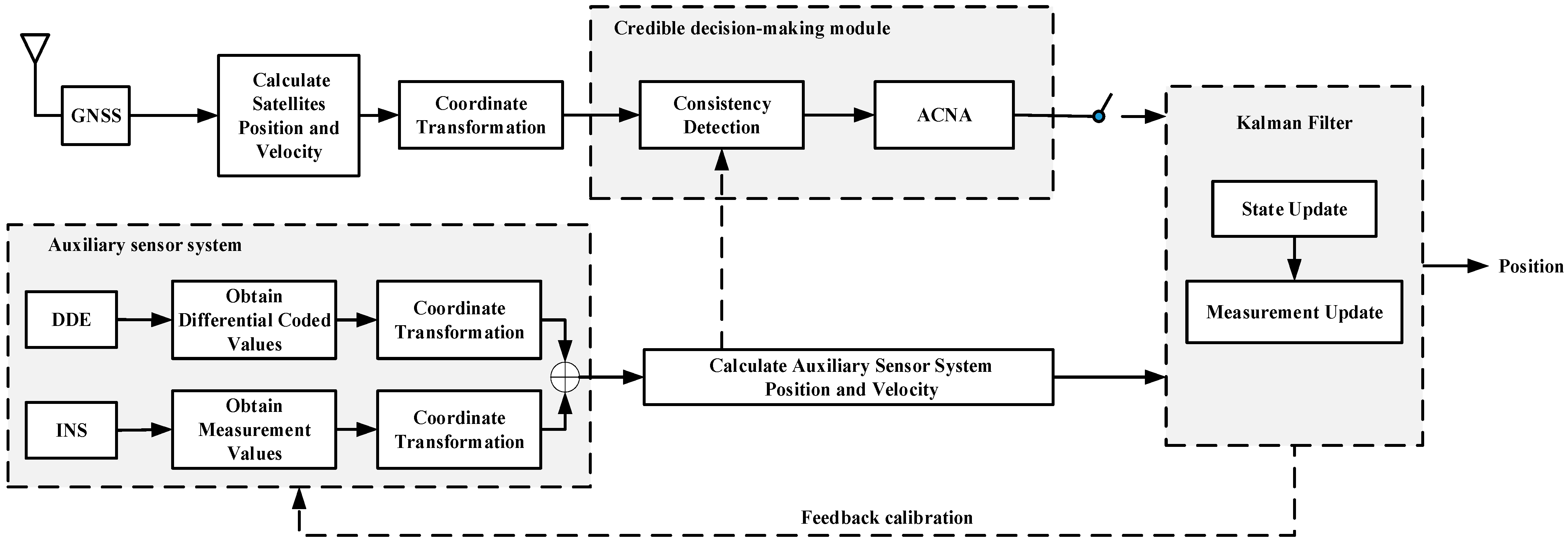
2. Credible Kalman Filter Model

2.1. Filter Model Description

In this paper, GNSS attacks are divided into two categories depending on their impact on the positioning domain: GNSS jump attacks and GNSS slow-change attacks. GNSS jump attacks happen when the GNSS is jammed or spoofed, causing invalid or large deviation in the positioning result. This type of GNSS attack is relatively easy to recognize, including GNSS jamming attacks, GNSS-generated attacks and GNSS repeater attacks. GNSS slow-change attacks happen when the positioning result drifts off slowly after the GNSS spoofing attack. This type of GNSS attack, including induced spoofing attacks, a not easy to identify. If the mobile terminal has suffered from a GNSS jump attack or a GNSS slow-change attack during movement, the new observation data will be abnormal, as mentioned above. With the feedback correction of the Kalman filter, the error will propagate and make the positioning results not credible [25]. This paper proposes a credible navigation algorithm based on an auxiliary sensor system, and a credible Kalman filtering framework (CKF) which includes an optimized Kalman filter framework with the addition of a credible decision-making module with two state-parameter update models (credible update model and auxiliary update model). Through sliding the credible-verification window, GNSS attacks that may occur in mobile terminals are continuously monitored, and the adaptive selection of the state-parameter update model is performed. If there is no attack alarm, the current GNSS signal is determined to be credible, and the credible update module is selected to perform position prediction, and state parameters are updated and corrected. If a GNSS attack warning does occur, it is determined to be untrusted, and the auxiliary update model is selected for position prediction. In the end, the credible navigation and positioning results are produced (see Section 3 in detail).

The credible Kalman filter framework is shown in Figure 1. In theory, the credible Kalman filter model can be applied to any kind of auxiliary sensor system that can provide the navigation position information (the auxiliary sensor system here includes IMUs, odometers, visual odometers, cameras, and other sensors that can provide absolute or relative position information. For example, the auxiliary navigation sensor could be an inertial navigation system (INS), a differential drive encoder (DDE) system or a DDE/INS integrated navigation system). In order to better explain the principle based on the self-developed credible navigation test terminal, this paper selects the DDE/INS-integrated navigation system as an auxiliary sensor system to derive the credible Kalman filter model. If other auxiliary navigation sensors are used instead, the credible Kalman filter model needs to be derived based on the corresponding sensor. The following is a theoretical modeling of the GNSS, DDE/INS auxiliary sensor system and credible Kalman filter.

2.2. GNSS Module

GNSS receivers generally use the WGS-84 ellipsoidal coordinate system [27] for coordinate representation, while the auxiliary sensor system generally uses the navigation coordinate system. In order to analyze the terminal position, the auxiliary sensor system in the mobile terminal and the GNSS location information must be put together in the same coordinate system. Therefore, it is necessary to transform the latitude, longitude and height information obtained from the GNSS in the geodetic coordinate system to the navigation coordinate system.

Assuming the latitude, longitude and height information of the starting position ${\rho }_0$ is $(b_0,l_0,h_0)$, where $b_0$ is the latitude, $l_0$ is the longitude, and $h_0$ is the height. Then, the position of ${\rho }_0$ transformed into the WGS-84 coordinate system is $(X_0,Y_0,Z_0)$. In the navigation coordinate system, the moving position $\rho$ of the mobile terminal in the geodetic coordinate system is $(b,l,h)$, and the position $\rho$ transformed into the navigation coordinate system is $(e^{\mathrm{G}},n^{\mathrm{G}},u^{\mathrm{G}})$. The major axis of the ellipsoid model is $a=\mathrm{6,378,137}\mathrm{km}$, and the oblateness is $e=1/298.257$. Then, the state parameter $x^{\mathrm{G}}$ of the GNSS model in the navigation coordinate system is

$$x^{\mathrm{G}}=\left[\begin{array}{c}{e}^{\mathrm{G}}\\ n^{\mathrm{G}}\\ u^{\mathrm{G}}\end{array}\right]=\left[\begin{array}{ccc}-\sin l_0& \cos l_0& 0\\ -\sin b_0\cdot \cos l_0& -\sin b_0\cdot \sin l_0& \cos b_0\\ cos{b}_0\cdot \cos l_0& \cos b_0\cdot \sin l_0& \sin b_0\end{array}\right]\left[\begin{array}{c}(a+h)\cdot \cos b\cdot \cos l-X_0\\ (a+h)\cdot \cos b\cdot \sin l-Y_0\\ (a\cdot (1-e^2)+h)\cdot \sin b-Z_0\end{array}\right].$$

(1)

2.3. DDE/INS System Module

The auxiliary sensor system needs to independently maintain the output position of the mobile terminal in the navigation coordinate system in order to verify the credibility of the GNSS positioning result. The auxiliary sensor system used in this paper is the DDE/INS auxiliary sensor system. The working principle of the DDE/INS system is shown in Figure 2.

Given the initial position, the DDE/INS system will calculate the position and heading of the mobile terminal through the DDE odometer. Before deriving the DDE/INS system model, we should derive the DDE system module first. The two wheels of the DDE odometer are independently controlled to realize the movement and steering control of the chassis [28]. By collecting the encoded data of the two wheels in a DDE unit time slot $\Delta t^{\mathrm{D}}$, the relative displacement in the navigation coordinate system can be solved as $(\Delta e_{}^{\mathrm{D}},\Delta n_{}^{\mathrm{D}},\Delta ya{w}^{\mathrm{D}})$. The moving distance of the left and right wheels in $\Delta t$ is denoted as $(s_k^{\mathrm{l}},s_k^{\mathrm{r}})$. Then, in the navigation coordinate system, the calculation model of $(s_k^{\mathrm{l}},s_k^{\mathrm{r}})$ is

$$\begin{array}{l}{s}_k^{\mathrm{l}}=o_{k-1,k}^{\mathrm{l}}\cdot 2\pi \cdot W_{\mathrm{r}}\cdot L_{\mathrm{l}}\\ s_k^{\mathrm{r}}=o_{k-1,k}^{\mathrm{r}}\cdot 2\pi \cdot W_{\mathrm{r}}\cdot L_{\mathrm{r}}\end{array}$$

(2)

where $(o_{k-1,k}^{\mathrm{l}},o_{k-1,k}^{\mathrm{r}})$ is the increment of the left and right wheels in $\Delta t^{\mathrm{D}}$, $(L_{\mathrm{l}},L_{\mathrm{r}})$ is the maximum count per rotation of the left or right wheel, $W_{\mathrm{r}}$ is the radius of the wheel, and $L_{\mathrm{w}}$ is the distance between the two wheels. Therefore, the navigation coordinate $(e_k^{\mathrm{D}},n_k^{\mathrm{D}})$ and yaw angle $ya{w}_k^{\mathrm{D}}$ at time k in the DDE system model is

$$\begin{array}{l}{e}_k^{\mathrm{D}}=e_{k-1}^{\mathrm{D}}+\frac{1}{2}\cdot (s_k^{\mathrm{l}}+s_k^{\mathrm{r}})\cdot \sin (ya{w}_{k-1}^{\mathrm{D}}+\frac{(s_k^{\mathrm{l}}-s_k^{\mathrm{r}})}{L_{\mathrm{w}}})\\ n_k^{\mathrm{D}}=n_{k-1}^{\mathrm{D}}+\frac{1}{2}\cdot (s_k^{\mathrm{l}}+s_k^{\mathrm{r}})\cdot \cos (ya{w}_{k-1}^{\mathrm{D}}+\frac{(s_k^{\mathrm{l}}-s_k^{\mathrm{r}})}{L_{\mathrm{w}}})\\ ya{w}_k^{\mathrm{D}}=ya{w}_{k-1}^{\mathrm{D}}+\frac{(s_k^{\mathrm{l}}-s_k^{\mathrm{r}})}{L_{\mathrm{w}}}\end{array}.$$

(3)

However, the DDE system model is greatly affected if the road surface is not flat, which causes a large error in the mileage calculation. In order to improve the navigation performance of the auxiliary sensor system and the credibility of the ACNA algorithm, the DDE system model is optimized by tightly coupling the yaw angle $ya{w}_{}^{\mathrm{I}}$ and the height $\Delta u_{}^{\mathrm{I}}$ calculated by INS, as shown in the following formula:

$$\begin{array}{l}{e}_k^{\mathrm{DI}}=e_{k-1}^{\mathrm{DI}}+\frac{1}{2}\cdot (s_k^{\mathrm{l}}+s_k^{\mathrm{r}})\cdot \sin (ya{w}_k^{\mathrm{I}})\\ n_k^{\mathrm{DI}}=n_{k-1}^{\mathrm{DI}}+\frac{1}{2}\cdot (s_k^{\mathrm{l}}+s_k^{\mathrm{r}})\cdot \cos (ya{w}_k^{\mathrm{I}})\\ u_k^{\mathrm{DI}}=u_{k-1}^{\mathrm{DI}}+\Delta u_k^{\mathrm{I}}\end{array}$$

(4)

where $(e_k^{\mathrm{DI}},n_k^{\mathrm{DI}},u_k^{\mathrm{DI}})$, $ya{w}_k^{\mathrm{I}}$ and $\Delta u_k^{\mathrm{I}}$ are the navigation coordinate, the yaw angle and the height at time k in the DDE/INS system.

In the navigation coordinate system, the velocity components $(v_x,v_y,v_z)$ of the mobile terminal in the east and north directions at time k is

$$\begin{array}{l}{v}_{x,k}=\frac{1}{2\Delta t^{\mathrm{D}}}\cdot (s_k^{\mathrm{l}}+s_k^{\mathrm{r}})\cdot \sin (ya{w}_k^{\mathrm{I}})\\ v_{y,k}=\frac{1}{2\Delta t^{\mathrm{D}}}\cdot (s_k^{\mathrm{l}}+s_k^{\mathrm{r}})\cdot \cos (ya{w}_k^{\mathrm{I}})\\ v_{z,k}=\frac{1}{\Delta t^{\mathrm{D}}}\cdot \Delta u_k^{\mathrm{I}}\end{array}$$

(5)

Therefore, the state parameter $x^{\mathrm{DI}}$ of the DDE/INS system model is

$$x^{\mathrm{DI}}=\left[\begin{array}{l}{e}_k^{\mathrm{DI}}\\ n_k^{\mathrm{DI}}\\ u_k^{\mathrm{DI}}\end{array}\right]=\left[\begin{array}{l}{e}_{k-1}^{\mathrm{DI}}+v_{x,k-1}\cdot \Delta t^{\mathrm{D}}\\ n_{k-1}^{\mathrm{DI}}+v_{y,k-1}\cdot \Delta t^{\mathrm{D}}\\ u_{k-1}^{\mathrm{DI}}+v_{z,k-1}\cdot \Delta t^{\mathrm{D}}\end{array}\right].$$

(6)

2.4. Credible Kalman Filter Model

The state parameter of the CKF filter system based on the DDE/INS system is

$$x={[x,y,z,v_x,v_y,v_z]}^{\mathrm{T}}$$

(7)

where $(x,y,z)$ is the navigation coordinate of the mobile terminal, while $(v_x,v_y,v_z)$ is the velocity of the mobile terminal. Then, the state update model ${x_k}^{\prime }$ at time k of the DDE/INS system is

$${x_k}^{\prime }=\left[\begin{array}{c}{x}_k\\ \begin{array}{l}{y}_k\\ z_k\end{array}\\ v_{x,k}\\ \begin{array}{l}{v}_{y,k}\\ v_{z,k}\end{array}\end{array}\right]=\left[\begin{array}{c}{x}_{k-1}+v_{x,k-1}\cdot \Delta t^{\mathrm{D}}\\ \begin{array}{l}{y}_{k-1}+v_{y,k-1}\cdot \Delta t^{\mathrm{D}}\\ z_{k-1}+v_{z,k-1}\cdot \Delta t^{\mathrm{D}}\end{array}\\ v_{x,k-1}\\ \begin{array}{l}{v}_{y,k-1}\\ v_{z,k-1}\end{array}\end{array}\right]={x_{k-1}}^{\prime }+\Delta t^{\mathrm{D}}\cdot \left[\begin{array}{c}{v}_{x,k-1}\\ \begin{array}{l}{v}_{y,k-1}\\ v_{z,k-1}\end{array}\\ 0\\ \begin{array}{l}0\\ 0\end{array}\end{array}\right]$$

(8)

If the GNSS information is determined to be credible, the GNSS state parameter $x^{\mathrm{G}}$ and the DDE/INS state parameters $x^{\mathrm{DI}}$ are used as observations of the CKF filter system to generate a credible update model A. In the update process of the CKF filter system, the measurement vector $Z^{\mathrm{A}}$ is expressed as

$$Z^{\mathrm{A}}={[e_k^{\mathrm{DI}},n_k^{\mathrm{DI}},u_k^{\mathrm{DI}},ya{w}_k^{\mathrm{I}},e_k^{\mathrm{G}},n_k^{\mathrm{G}},u_k^{\mathrm{G}}]}^{\mathrm{T}}.$$

(9)

If the GNSS information is determined to be untrusted, the CKF filter system shields the GNSS state parameter $x^{\mathrm{G}}$, and only uses the DDE/INS state parameters $x^{\mathrm{DI}}$ to generate an auxiliary update model V. Then, it enters the CKF filter system update process, in which the measurement vector $Z^{\mathrm{V}}$ is expressed as

$$Z^{\mathrm{V}}={[e_k^{\mathrm{DI}},n_k^{\mathrm{DI}},u_k^{\mathrm{DI}},ya{w}_k^{\mathrm{I}}]}^{\mathrm{T}}.$$

(10)

3. Credible Navigation Algorithm

3.1. Algorithm Model

By setting the size of the credible verification threshold and the size of the credible verification window, the ACNA algorithm monitors GNSS drift, effectively identifies GNSS jump/slow attack, and improves the credibility of the system. The definitions of GNSS drift, credible verification window and credible verification threshold are given below.

GNSS drift: The offset of the GNSS positioning result relative to the positioning result of the auxiliary sensor system. The GNSS drift $\Delta {\rho }_k$ at time k is

$$\Delta {\rho }_k=\sqrt{{(e_k^{\mathrm{G}}-e_k^{\mathrm{DI}})}^2+{(n_k^{\mathrm{G}}-n_k^{\mathrm{DI}})}^2+{(u_k^{\mathrm{G}}-u_k^{\mathrm{DI}})}^2}.$$

(11)

Credible verification window: The credibility of GNSS is determined using the credible verification window as a scope of judgment. During the process of credibility determination, the drift $\Delta \rho$ over several consecutive positioning time slots is analyzed to determine whether the GNSS signal is credible. The number of consecutive positioning time slots mentioned above is in fact the size of the credible verification window. The credible verification window includes the jump verification window $n_{\mathrm{j}}$, and the slow-change verification window $n_{\mathrm{s}}$. Here, $n_{\mathrm{j}}$ is used to verify whether the GNSS has experienced a GNSS jump attack while $n_{\mathrm{s}}$ is used to verify whether the GNSS has experienced a GNSS slow-change attack. In the credibility determination process, the credibility verification window will continue to slide over time.

Credible verification threshold: During the movement of the mobile terminal, the trajectories of two adjacent points are correlated. The possible position range of the mobile terminal at time k + 1 can be predicted according to the position at time k, the velocity at time k, the yaw angle at time k and the measurement error of GNSS and the auxiliary sensor system from time k to time k + 1. The GNSS signal lies within a certain error range: if it exceeds a certain error range, the GNSS signal can be considered abnormal. At this point, the radius of the abnormal position beyond the certain error range is set as the credible threshold. During the determination of the credible verification window, it is required to keep monitoring whether GNSS drift exceeds a certain threshold. This threshold is defined as the credible verification threshold. Our method sets separate thresholds for GNSS jump attacks and GNSS slow-change attacks as $T{h}_{\mathrm{j}}$ and $T{h}_{\mathrm{s}}$.

If the signal continues to be abnormal, GNSS jump/slow-change attack can be detected based on the analysis of measurement information in the credible verification window range. If the credibility verification threshold is too high, a missing alarm may be triggered. If the credible verification threshold is too low, a false alarm may be triggered. If there is only one or two signal abnormalities within a certain period of time, it may be a “GNSS signal false point”, which may be caused by other factors. In order to remove these unwanted signal fluctuations, appropriate parameter values need to be set to filter them out to effectively eliminate false points, improve the accuracy and reduce the false/missing alarm rate of the system.

According to the state and prediction location results of ACNA, the location of points is divided into four categories: (1) $TP$: predict as normal, in fact normal, (2) $FP$: predict as normal, in fact abnormal, (3) $TN$: predict as abnormal, in fact abnormal, (4) $FN$: predict as abnormal, in fact normal. Then, the accuracy rate of navigation prediction $P_{\mathrm{D}}$ is

$$P_{\mathrm{D}}=\frac{TP+TN}{TP+FN+FP+TN}.$$

(12)

The false alarm rate $P_{\mathrm{FA}}$ is

$$P_{\mathrm{FA}}=\frac{FP}{FP+TN}.$$

(13)

The missing alarm rate $P_{\mathrm{MD}}$ is

$$P_{\mathrm{MD}}=\frac{FN}{TP+FN}.$$

(14)

In order to improve the credibility of the ACNA algorithm, it is necessary to set the appropriate credible verification threshold and credible verification window. According to the minimum error criterion [29], minimizing the sum of integrity and availability risks can maximize the accuracy of the navigation algorithm. Therefore, this then becomes an optimization problem. The optimization objective is to maximize the accuracy rate of the algorithm and minimize the false alarm rate and missing alarm rate of the algorithm. That is:

$$\max (P_{\mathrm{D}})\wedge \min (P_{\mathrm{FA}}+P_{\mathrm{MD}})$$

$$\mathrm{s}.\mathrm{t}.$$

$$n_{\mathrm{j}}>1$$

(15)

$$n_{\mathrm{s}}>n_{\mathrm{j}}$$

(16)

$$T{h}_{\mathrm{j}}\ge {\sigma }^{\mathrm{G}}$$

(17)

$$T{h}_{\mathrm{j}}\le 3{\sigma }^{\mathrm{G}}$$

(18)

$$T{h}_s\ge {\sigma }^{\mathrm{G}}$$

(19)

$$T{h}_s\le 3{\sigma }^{\mathrm{G}}$$

(20)

$$T{h}_s\ge {\displaystyle \sum _{i=k-n_s+1}^k{\epsilon }_i^{\mathrm{DI}}}{\displaystyle /}{n}_s.$$

(21)

Equations (15) and (16) are credible verification window constraints. The jump attack of GNSS means that the GNSS drift exceeds the jump verification threshold for $n_{\mathrm{j}}$ consecutive moments. The jump attack detection method can be used to detect the “GNSS signal false points” of the system, improve the accuracy rate, and reduce the false alarm rate. Therefore, $n_{\mathrm{j}}$ should satisfy $n_{\mathrm{j}}>1$. The slow-change verification window $n_{\mathrm{s}}$ is used after the jump attack detection. Therefore, $n_{\mathrm{s}}$ is set to be larger than the jump verification window $n_{\mathrm{j}}$ to optimize the algorithm running time.

Equations (17)–(21) are credible verification threshold constraints. The GNSS positioning solution follows a Gaussian distribution, with the mean and standard deviation being ${\mu }^{\mathrm{G}}$ and ${\sigma }^{\mathrm{G}}$. According to the Pauta criterion ($3\sigma$ criterion), the possibility that the GNSS positioning solution exceeds the range $(\mu -3\sigma ,\mu +3\sigma )$ is only 0.27%. Thus, an error of ±$3\sigma$ can be used as the limit error of the GNSS positioning settlement result. To identify GNSS jump attack, the choice of $T{h}_{\mathrm{j}}$ should not exceed the limit error of GNSS at $3{\sigma }^{\mathrm{G}}$. At the same time, to ensure the positioning accuracy of the system, $T{h}_{\mathrm{j}}$ should not be lower than the GNSS error at ${\sigma }^{\mathrm{G}}$. Thus, $T{h}_{\mathrm{j}}$ should satisfy Equations (17) and (18).

As for the slow-change attack of GNSS, the location domain changes by only a small amount per unit time, which is difficult to detect by jump verification. The selection of $T{h}_{\mathrm{s}}$ should be greater than the measurement error of the GNSS system and the cumulative measurement error of the auxiliary sensor system. At each unit time in the credible verification window, the measurement errors of the GNSS system are relatively independent, and they all satisfy the $3\sigma$ principle. $T{h}_{\mathrm{s}}$ should not be lower than the GNSS error at ${\sigma }^{\mathrm{G}}$ and not exceed the limit error of GNSS at $3{\sigma }^{\mathrm{G}}$ during the slow-change verification window $n_{\mathrm{s}}$. Thus, $T{h}_{\mathrm{s}}$ should satisfy Equations (19) and (20). The cumulative measurement error of the auxiliary sensor system $P_{}^{\mathrm{DI}}$ is the cumulative measurement error of the auxiliary sensor system during the credible verification window. The measurement error of the auxiliary sensor system will continue to accumulate if there is no GNSS observation to correct and calibrate the auxiliary sensor system. Therefore, $P_{}^{\mathrm{DI}}$ can be calculated as

$$P_{{}_{k-n_s+1},\cdots {,}_{k-1}{,}_k}^{\mathrm{DI}}={\displaystyle \sum _{i=k-n_s+1}^k{\epsilon }_i^{\mathrm{DI}}}$$

(22)

where ${\epsilon }_i^{\mathrm{DI}}$ is the measurement error of the auxiliary sensor system at time $i$. Then, $T{h}_{\mathrm{s}}$ should be greater than the average cumulative error of the auxiliary sensor system to accurately determine whether a GNSS attack occurs, as described in Equation (21). In order to simplify the measurement error model of the auxiliary sensor system, we make the following assumptions for the error model. The measurement errors of the auxiliary sensor system ${\epsilon }_{}^{\mathrm{DI}}$ all have the same normal distribution, with a mean of ${\mu }^{\mathrm{DI}}$ and a variance of ${\sigma }_{\mathrm{DI}}^2$. That is

$$\begin{array}{l}E({\epsilon }_k^{\mathrm{DI}})={\mu }^{\mathrm{DI}}\\ V({\epsilon }_k^{\mathrm{DI}})={\sigma }_{\mathrm{DI}}^2\end{array}$$

(23)

At each unit time in the credible verification window, the measurement errors of the auxiliary sensor system are relatively independent; thus, the measurement errors of the auxiliary sensor system can be simplified as:

$$P_{{}_{k-n_s+1},\cdots {,}_{k-1}{,}_k}^{\mathrm{DI}}={\sigma }_{\mathrm{DI}}^2\times n_s.$$

(24)

3.2. Algorithm Design

According to the optimization theoretical model above, we designed the ACNA method to detect whether the GNSS was subjected to jump or slow-change attacks, based on whether the GNSS drift exceeds the credible verification threshold within the credible verification window. In order to maximize the accuracy of the algorithm and minimize the risk of algorithm integrity and availability, the updated model of the filter was selected adaptively to obtain the credible navigation prediction.

At time k, when the mobile terminal has a positioning requirement, it receives the GNSS signal and calculates the position of the mobile terminal as ${\rho }_k^{\mathrm{G}}$. At this time, the estimated position obtained from the auxiliary sensor system is ${\rho }_k^{\mathrm{DI}}$

$$\begin{array}{l}{\rho }_k^{\mathrm{G}}=[e_k^{\mathrm{G}},n_k^{\mathrm{G}},u_k^{\mathrm{G}}]\\ {\rho }_k^{\mathrm{DI}}=[e_k^{\mathrm{DI}},n_k^{\mathrm{DI}},u_k^{\mathrm{DI}}]\end{array}$$

(25)

After acquiring the GNSS signal in the current positioning time slot, ACNA enters the GNSS interruption verification stage in order to determine whether the GNSS signal acquired is valid. If the GNSS signal is invalid (${\rho }_k^{\mathrm{G}}=V$ and V means the signal is invalid) at this time, it is concluded that the GNSS signal is interrupted, and the system sends a GNSS signal interruption alarm to the mobile terminal. Then, the auxiliary updated model is selected to filter and update the position prediction until the GNSS is determined to be valid (${\rho }_k^{\mathrm{G}}\ne V$). After that, the data of GNSS and auxiliary sensor system are extracted and processed, and the jump attack detection stage is entered.

In the GNSS jump attack detection stage, the credibility of the GNSS positioning results can be verified through $\Delta {\rho }_{\mathrm{k}}$, $n_{\mathrm{j}}$, and $T{h}_{\mathrm{j}}$. For the consecutive positioning time slots $n_{\mathrm{j}}$, the GNSS drift $\Delta \rho$ should be determined between each positioning time slot. The jump mark ${\mathrm{flag}}_{\mathrm{j}}$ tracks and records the GNSS signal jump, as

$${\mathrm{flag}}_{\mathrm{j}}(k)=\{\begin{array}{l}{\mathrm{flag}}_{\mathrm{j}}(k-1)+1\hspace{1em}\hspace{1em}\Delta {\rho }_{\mathrm{k}}>T{h}_{\mathrm{j}}\\ 0\hspace{1em}\hspace{1em}\Delta {\rho }_{\mathrm{k}}\le T{h}_{\mathrm{j}}\end{array}.$$

(26)

If ${\mathrm{flag}}_{\mathrm{j}}(k)\ge n_{\mathrm{j}}$, it is verified that a GNSS jump attack has occurred, as shown in Figure 3. At this time, GNSS is judged to be in the untrusted stage, and the auxiliary update model is selected for terminal position prediction, and a jump alarm was issued at the same time.

If no GNSS jump attack occurs, the algorithm enters the GNSS slow-change verification stage, and the GNSS positioning result is verified based on $\Delta {\rho }_{\mathrm{k}}$, $n_s$ and $T{h}_{\mathrm{s}}$. For the consecutive positioning time slots $n_{\mathrm{s}}$, the GNSS drift $\Delta \rho$ in each slot should be tracked and recorded by the slow-change mark ${\mathrm{flag}}_{\mathrm{s}}$. At time $k$, ${\mathrm{flag}}_{\mathrm{s}}\left(k\right)$ represents the statistical average of GNSS drift from time $k+1-n_s$ to $k$, as

$${\mathrm{flag}}_{\mathrm{s}}(k)={\displaystyle \sum _{i=1}^{n_s}\Delta {\rho }_{k+i-n_s}}/n_s.$$

(27)

If ${\mathrm{flag}}_{\mathrm{s}}\left(k\right)\ge T{h}_{\mathrm{s}}$, it is verified that GNSS drift exceeds the threshold from time $k-n_s$ to $k$ during the slow-change verification window, which means a GNSS slow-change attack may occur, as shown in Figure 4. At this time, GNSS is judged to be in an untrusted stage, and the auxiliary update model is selected for terminal position prediction, and at the same time, a slow-change alarm is issued.

If there is no interruption or jump/slow-change attack on the GNSS signal, the GNSS is judged to be in a credible stage, and the credible update model is selected for the filtering update and position prediction.

The algorithm flowchart is presented in Figure 5 and the logical flow of the algorithm is explained as follows:

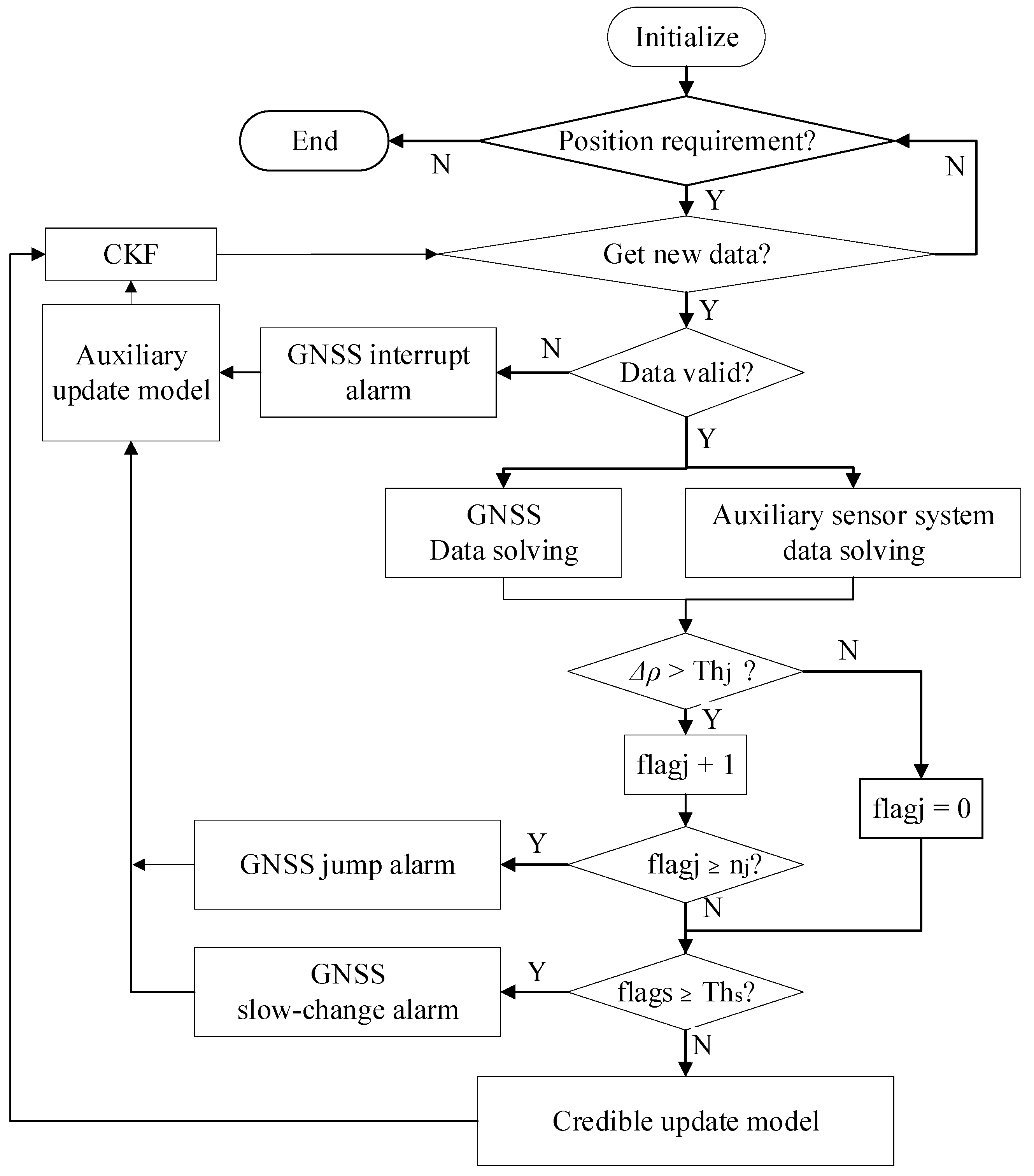
• Step 1: Initialization. Set the initial global position (converted to the navigation coordinate system) according to the GNSS signal acquired when the mobile terminal is initially at stationary. Initialize parameters $n_{\mathrm{j}}$, $T{h}_{\mathrm{j}}$, $n_{\mathrm{s}}$, $T{h}_{\mathrm{s}}$, ${\mathrm{flag}}_{\mathrm{j}}$ and ${\mathrm{flag}}_{\mathrm{s}}$.
• Step 2: Decide whether there is a navigation and positioning requirement. If so, the GNSS receiver and auxiliary sensor will enter the working state and go to step 3; otherwise, go to step 8.
• Step 3: Determine whether the GNSS and auxiliary sensor system have new and valid input data. If the acquired information of GNSS and auxiliary sensor system is valid, the information of GNSS from global coordinates is converted to navigation coordinates, and the position unity with the auxiliary sensor system is realized to obtain ${\rho }_k^{\mathrm{G}}$ and ${\rho }_k^{\mathrm{DI}}$. Then, we go to step 4; if the effective information of the auxiliary navigation sensor system is obtained, and the GNSS positioning result is interrupted, the auxiliary update model is used to maintain the terminal position prediction, and we go to step 3 again; if no valid information is obtained, we go back to step 2.
• Step 4: Calculate GNSS drift $\Delta {\rho }_k$ at time k. If $\Delta {\rho }_k>T{h}_{\mathrm{j}}$, then we have ${\mathrm{flag}}_{\mathrm{j}}(k-1)+1$, and we go to step 5; otherwise, we have ${\mathrm{flag}}_{\mathrm{j}}(k)=0$, and we go to step 6.
• Step 5: Determine the size of ${\mathrm{flag}}_{\mathrm{j}}(k)$. If ${\mathrm{flag}}_{\mathrm{j}}(k)<{\mathrm{n}}_{\mathrm{j}}$, we proceed to Step 6; if ${\mathrm{flag}}_{\mathrm{j}}(k)\ge {\mathrm{n}}_{\mathrm{j}}$, it is determined that there is a GNSS jump attack, the GNSS is set as an untrusted navigation source, and the auxiliary update model is used to maintain the terminal position prediction at this time. If this happens, we reverse back to step 3.
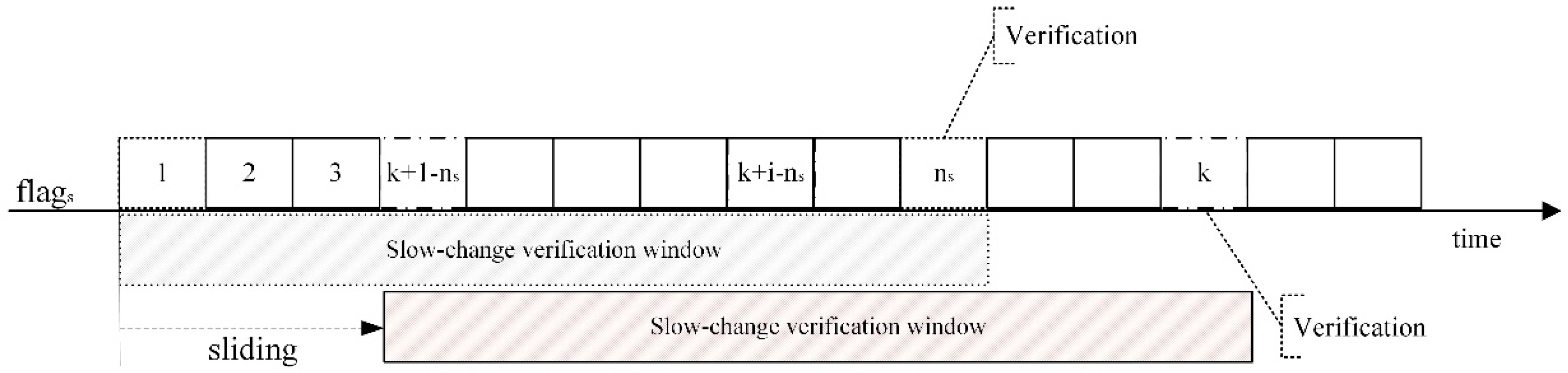
• Step 6: Calculate ${\mathrm{flag}}_{\mathrm{s}}(k)$. If ${\mathrm{flag}}_{\mathrm{s}}\left(k\right)\ge T{h}_{\mathrm{s}}$, it is determined that there is a GNSS slow-change attack, the GNSS is set as an untrusted navigation source, and the auxiliary update model is used to maintain the terminal position prediction. Then, we go back to step 3; otherwise, we continue to step 7.
• Step 7: GNSS is in a credible stage. The credible update model is used to maintain the terminal position output, and then we go to step 3 again.
• Step 8: End.

4. Performance Evaluation

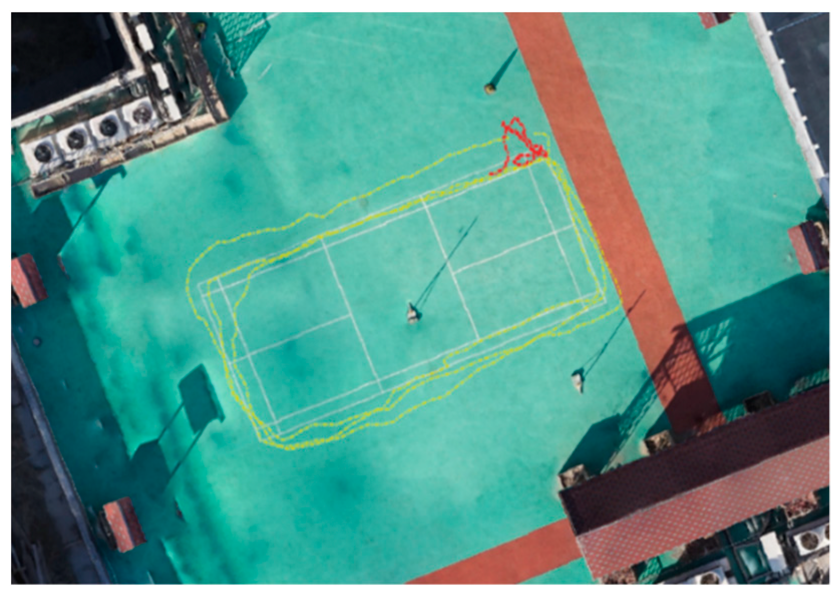
4.1. Experimental Platform and Data Set

In order to test the proposed ACNA algorithm, simulations and evaluations are performed on two data sets collected during the real driving. The experiment is conducted using a self-designed robot system named QJ-Racecar equipped with RTK, GNSS, INS and DDE sensors. Its mechanical structure and sensors are shown in Figure 6. Additionally, the sensor specifications are shown in

Table 1. List of sensor simulation parameters.

Sensor	Model	Sensor Error	Sample Rate
RTK	MXT906A	Horizontal position accuracy RTK 0.025 m	1 Hz
GNSS	NEO-6M	Horizontal position accuracy GPS 2.5 m	1 Hz
Accelerometer	MPU9250	Noise power Spectral Density $300 \mathsf{\mu }\mathrm{g}/\sqrt{\mathrm{Hz}}$	10 Hz
Gyroscope	MPU9250	Rate Noise Spectral Density $0.01°/\mathrm{s}/\sqrt{\mathrm{Hz}}$	10 Hz
Magnetometer	MPU9250	Sensitivity Scale Factor $0.6 \mathsf{\mu }\mathrm{T}/\mathrm{LSB}$	10 Hz
DDE	JGB37-520	Max Encoder 495	10 Hz

below.

Two data sets are collected during the test ride. Data set 1 is named ${\Psi }_1$, and it shows an outdoor static test of the mobile terminal with a 5 min duration. This data set also provides the initial position of the mobile terminal, as shown in

Table 2. Initial state parameters of the trajectory.

Type	Initial State of the Trajectory
Lan/Lon/Height	40.0702° N/116.2747° E/54.63 m
Heading/Roll/Yaw	0°, 0°, 248°

below. Data set 2 is named ${\Psi }_2$, and it is collected by driving the robot along the sidelines of a 13.4 m long and 6.1 m wide badminton field at an average speed of 0.5 m/s. The trajectories of the two data sets exported by the RTK receiver are shown in Figure 7 and the number of available satellites during driving is shown in Figure 8.

4.2. Simulation Results

In order to validate the performance of the proposed algorithm ACNA, the GNSS jump or slow-change attacks are simulated on the data set ${\Psi }_1$ and ${\Psi }_2$. The simulation of GNSS jump attacks are applied to ${\Psi }_2$ to obtain ${\tilde{\Psi }}_2$. The simulation of GNSS slow-change attacks are applied to ${\Psi }_2$ to obtain ${\tilde{\Psi }}_3$. Additionally, the simulation of GNSS jump and slow-change attacks are applied to ${\Psi }_2$ to obtain ${\tilde{\Psi }}_4$.

GNSS jump attacks are injected into data set as follows:

$${\tilde{\rho }}_{}^{\mathrm{GJ}}={\rho }_{}^{\mathrm{G}}+\Delta {\rho }_{}^{\mathrm{J}},\forall \Delta {\rho }_{}^{\mathrm{J}}\sim N(20,0.1)$$

(28)

where ${\tilde{\rho }}_{}^{\mathrm{GJ}}$ represents the position after GNSS jump attacks are injected, ${\rho }_{}^{\mathrm{G}}$ represents the GNSS position, and $\Delta {\rho }_{}^{\mathrm{J}}$ (random interference is added with an average of 20 m and a variance of 0.1) represents the position disturbance caused by GNSS jump attacks in the location domain. As can be seen from Equation (28), the jump attack injects big errors to GNSS signals.

GNSS slow-change attacks are injected into data set as follows:

$${\tilde{\rho }}_{}^{\mathrm{GS}}={\rho }_{}^{\mathrm{G}}+{\displaystyle \sum _{i=T}^{}\Delta {\rho }_i^{\mathrm{S}}},\forall \Delta {\rho }_{}^{\mathrm{S}}\sim N(0.5,0.05)$$

(29)

where ${\tilde{\rho }}_{}^{\mathrm{GS}}$ represents the position after GNSS slow-change attacks are injected, and $\Delta {\rho }_i^{\mathrm{S}}$ (random interference is superimposed per second with an average of 0.5 m and a variance of 0.05) represents the positional disturbance at time i generated by GNSS slow-change attacks in the location domain. As can be seen from Equation (29), the slow-change attack injects small errors to GNSS signals slowly and continuously during each second.

Under such a condition, slowly injected errors can influence the filter gradually. In GNSS jump attack simulation (data set ${\tilde{\Psi }}_2$), the segment from 150 s to 300 s of the data set is exposed to GNSS jump attacks defined in Equation (28). In GNSS slow-change attack simulation (data set ${\tilde{\Psi }}_3$), the segment from 150 s to 300 s of the data set is exposed to GNSS slow-change attacks defined in Equation (29). Additionally, in the jump and slow-change attack simulation (data set ${\tilde{\Psi }}_4$), the segment from 50 s to 100 s of the data set is exposed to GNSS jump attacks defined in Equation (28) and the segment from 150 s to 200 s of the data set is exposed to GNSS slow-change attacks defined in Equation (29).

4.3. Parameter Analysis

This section analyzes the impact of the jump parameter settings ($n_{\mathrm{j}}$ and $T{h}_{\mathrm{j}}$) and slow-change parameter settings ($n_{\mathrm{s}}$ and $T{h}_{\mathrm{s}}$) on $P_{\mathrm{D}}$ and $P_{\mathrm{FA}}+P_{\mathrm{MD}}$ mentioned in Section 3.1. First, we focus on the impact of jump parameter settings. Data set ${\tilde{\Psi }}_2$ is selected for analysis in order to shield the influence of slow-change parameter settings on $P_{\mathrm{D}}$, $P_{\mathrm{FA}}$ and $P_{\mathrm{MD}}$. According to Equations (16)–(18), the value range of $n_{\mathrm{j}}$ is set from 1 to 20, and the value range of $T{h}_{\mathrm{j}}$ is set as follows:

$$\begin{array}{l}T{h}_{\mathrm{j}}=0.1t \mathrm{m} \\ \mathrm{s}.\mathrm{t}. t=0~60\end{array}$$

(30)

The simulation results are shown in Figure 9. It can be seen that when $n_{\mathrm{j}}$ remains unchanged, with the increase in $T{h}_{\mathrm{j}}$, $P_{\mathrm{D}}$ becomes stable to 1 after its wavelike rising while $P_{\mathrm{FA}}+P_{\mathrm{MD}}$ becomes stable to 0 after its wavelike dropping.

Then, we set a parameter $f_{\mathrm{a}}$ in order to maximize the accuracy rate of the navigation algorithm, as follows:

$$f_{\mathrm{a}}=\max (P_{\mathrm{D}}).$$

(31)

At the same time, we set another parameter $f_{\mathrm{c}}$ to minimize the sum of the missing alarm rate $P_{\mathrm{MD}}$ and false alarm rate $P_{\mathrm{FA}}$ to evaluate the sum of integrity and availability risks, as follows:

$$f_{\mathrm{c}}=\min (P_{\mathrm{FA}}+P_{\mathrm{MD}}).$$

(32)

The simulation results are shown in Figure 10. The impact of $n_{\mathrm{j}}$ on $f_{\mathrm{a}}$ and $f_{\mathrm{c}}$ is analyzed in Figure 10a. It can be seen that as $n_{\mathrm{j}}$ increases, $f_{\mathrm{a}}$ is stable at 1, while $f_{\mathrm{c}}$ is stable at 0. No matter what the value of $n_{\mathrm{j}}$ is, the value of $f_{\mathrm{a}}$ and $f_{\mathrm{c}}$ remains the same. That is, the value of $P_{\mathrm{D}}$ would become to 1 and $P_{\mathrm{FA}}+P_{\mathrm{MD}}$ would become to 0 as the value of $T{h}_{\mathrm{j}}$ increases no matter what the value of $n_{\mathrm{j}}$ is. The difference is that $T{h}_{\mathrm{j}}$ is different when $P_{\mathrm{D}}$ increases to 1. Therefore, according to Equation (15), the jump parameter $n_{\mathrm{j}}$ is set to 2. Additionally, according to the trend of $P_{\mathrm{D}}$ and $P_{\mathrm{FA}}+P_{\mathrm{MD}}$ when $n_{\mathrm{j}}$ is set to 2, $T{h}_{\mathrm{j}}$ is set to 1.5 m, as shown in Figure 10b. Then, we will have $P_{\mathrm{D}}=100\%$ and $P_{\mathrm{FA}}+P_{\mathrm{MD}}=0\%$.

Next, the effect of the slow-change parameter on $P_{\mathrm{D}}$ and $P_{\mathrm{FA}}$ + $P_{\mathrm{MD}}$ is analyzed based on the data set ${\tilde{\Psi }}_3$. In this experiment, the value range of the slow-change verification window $n_{\mathrm{s}}$ is set to the range 1 to 20, and the value range of $T{h}_{\mathrm{s}}$ is set as follows:

$$\begin{array}{l}T{h}_{\mathrm{s}}=0.01t \mathrm{m} \\ \mathrm{s}.\mathrm{t}. t=0~1000\end{array}$$

(33)

The simulation results are shown in Figure 11 and Figure 12. In Figure 11, it can be seen that when the value of $n_{\mathrm{s}}$ is constant, with the increase in $T{h}_{\mathrm{s}}$, $P_{\mathrm{D}}$ becomes stable after its wavelike rising and $P_{\mathrm{FA}}+P_{\mathrm{MD}}$ becomes stable after its wavelike falling. According to Figure 12a, the influence of the slow-change verification window on $f_{\mathrm{a}}$ and $f_{\mathrm{c}}$ can be analyzed and reflected. In order to maximize the accuracy rate $P_{\mathrm{D}}$ and minimize $P_{\mathrm{FA}}+P_{\mathrm{MD}}$, we pick the slow-change parameters as $n_{\mathrm{s}}=5$ and $T{h}_{\mathrm{s}}=1.28 \mathrm{m}$. Then, we will have $P_{\mathrm{D}}=100\%$, and $P_{\mathrm{FA}}+P_{\mathrm{MD}}=0\%$, as shown in Figure 12b.

5. Experimental Analysis

In order to verify the performance of the ACNA algorithm, we try to compare it with the traditional extended Kalman filter method (EKF) [30] and the reduced IMU and odometer algorithm (RIO) [24]. The EKF algorithm uses the traditional EKF algorithm to fuse GPS and DDE/INS data with no GNSS verification process; that is, the updated measurement is the direct input of the Kalman filter for state update and position prediction. The RIO algorithm has distance constraints and can detect GNSS jump attacks. In the following passage, we compare the three algorithms using data set ${\tilde{\Psi }}_2$, ${\tilde{\Psi }}_3$ and ${\tilde{\Psi }}_4$.

5.1. Results of Data Set ${\tilde{\Psi }}_2$

Figure 13 shows the position error of ACNA, EKF and RIO under GNSS jump attacks (data set ${\tilde{\Psi }}_2$). After GNSS attacks in data set ${\tilde{\Psi }}_2$, the $1\sigma$ positioning accuracy of GNSS increases to 13.47 m. Figure 14 shows the corresponding movement trajectories of the three algorithms of ACNA, EKF and RIO under GNSS attacks. Their east, north and relative positioning accuracy (${\sigma }_{\mathrm{east}}$, ${\sigma }_{\mathrm{north}}$ and $\sigma$) and maximum error ($E_{\mathrm{MaxEast}}$, $E_{\mathrm{MaxNorth}}$ and $E_{\mathrm{Max}}$) are shown in

Table 3. East, north and relative positioning accuracy and maximum error of the three algorithms on data set ${\tilde{\Psi }}_2$.

Algorithm	$${\mathit{\sigma }}_{\mathbf{east}}/\mathbf{m}$$	$${\mathit{\sigma }}_{\mathbf{north}}/\mathbf{m}$$	$$\mathit{\sigma }/\mathbf{m}$$	$${\mathit{E}}_{\mathbf{MaxEast}}/\mathbf{m}$$	$${\mathit{E}}_{\mathbf{MaxNorth}}/\mathbf{m}$$	$${\mathit{E}}_{\mathbf{Max}}/\mathbf{m}$$
GNSS	10.17	9.88	13.47	21.11	20.83	29.42
EKF	9.92	9.80	13.24	21.08	20.83	28.89
RIO	1.21	1.86	1.39	2.48	5.79	5.80
ACNA	1.06	1.63	1.14	2.01	4.94	5.02

below.

It can be seen that the EKF algorithm fails to detect GNSS jump attacks and the positioning errors grows gradually as the GNSS attacks occur. The $1\sigma$ positioning accuracy of the EKF algorithm increases to 13.24 m, with an improvement of 2% compared with the GNSS. Additionally, the RIO algorithm and ACNA algorithm can detect jump attacks in time. The $1\sigma$ positioning accuracy of the RIO algorithm increases to 1.39 m, with an improvement of 90% compared with the GNSS. Additionally, the $1\sigma$ positioning accuracy of the ACNA algorithm increases at 1.14 m, with an improvement of 92% compared with the GNSS.

5.2. Results of Data Set ${\tilde{\Psi }}_3$

Figure 15 shows the position error of ACNA, EKF and RIO in the east and north directions after GNSS slow-change attacks (data set ${\tilde{\Psi }}_3$). After GNSS attacks on data set ${\tilde{\Psi }}_3$, the $1\sigma$ positioning accuracy of the GNSS increases to 34.27 m. Figure 16 shows the corresponding movement trajectory of the three algorithms under GNSS attacks. Their east, north and relative positioning accuracy (${\sigma }_{\mathrm{east}}$, ${\sigma }_{\mathrm{north}}$ and $\sigma$) and maximum error ($E_{\mathrm{MaxEast}}$, $E_{\mathrm{MaxNorth}}$ and $E_{\mathrm{Max}}$) are shown in

Table 4. The east, north and relative positioning accuracy and maximum error of the three algorithms in the data set ${\tilde{\Psi }}_3$.

Algorithm	$${\mathit{\sigma }}_{\mathbf{east}}/\mathbf{m}$$	$${\mathit{\sigma }}_{\mathbf{north}}/\mathbf{m}$$	$$\mathit{\sigma }/\mathbf{m}$$	$${\mathit{E}}_{\mathbf{MaxEast}}/\mathbf{m}$$	$${\mathit{E}}_{\mathbf{MaxNorth}}/\mathbf{m}$$	$${\mathit{E}}_{\mathbf{Max}}/\mathbf{m}$$
GNSS	24.69	24.55	34.27	76.39	75.97	107.73
EKF	23.56	23.52	32.76	73.33	73.52	103.84
RIO	5.14	5.44	6.77	11.76	13.75	17.06
ACNA	1.07	1.66	1.17	2.01	5.05	5.12

below.

It can be seen from the results that EKF is unable to detect GNSS slow-change attacks and its $1\sigma$ positioning accuracy increases to 32.76 m, with an improvement of 4% compared with the GNSS. The RIO algorithm detects slow-change attacks after it occurs for 26 s. Therefore, its $1\sigma$ positioning accuracy increases to 6.77 m, which is improved by 80% compared with GNSS. On the other hand, the ACNA algorithm can detect GNSS slow-change attacks in time and its $1\sigma$ positioning accuracy is 1.17 m, with an improvement of 97% compared with the GNSS.

5.3. Results of Data Set ${\tilde{\Psi }}_4$

Figure 17 shows the position error of ACNA, EKF and RIO after GNSS jump and slow-change attacks (data set ${\tilde{\Psi }}_4$). After GNSS attacks on data set ${\tilde{\Psi }}_4$, the $1\sigma$ positioning accuracy of the GNSS increases to 11.80 m. Figure 18 shows the corresponding movement trajectory of the three algorithms under GNSS attacks. Their east, north and relative positioning accuracy (${\sigma }_{\mathrm{east}}$, ${\sigma }_{\mathrm{north}}$ and $\sigma$) and maximum error ($E_{\mathrm{MaxEast}}$, $E_{\mathrm{MaxNorth}}$ and $E_{\mathrm{Max}}$) are shown in

Table 5. The east, north and relative positioning accuracy and maximum error of the three algorithms in the data set ${\tilde{\Psi }}_4$.

Algorithm	$${\mathit{\sigma }}_{\mathbf{east}}/\mathbf{m}$$	$${\mathit{\sigma }}_{\mathbf{north}}/\mathbf{m}$$	$$\mathit{\sigma }/\mathbf{m}$$	$${\mathit{E}}_{\mathbf{MaxEast}}/\mathbf{m}$$	$${\mathit{E}}_{\mathbf{MaxNorth}}/\mathbf{m}$$	$${\mathit{E}}_{\mathbf{Max}}/\mathbf{m}$$
GNSS	8.67	8.78	11.80	25.34	24.70	35.39
EKF	7.80	8.04	10.65	22.89	22.41	32.03
RIO	5.11	5.40	6.75	12.01	13.93	17.37
ACNA	0.78	0.97	0.81	2.01	3.38	3.38

below.

It can be seen from the results that EKF is unable to detect GNSS jump attacks or slow-change attacks and its $1\sigma$ positioning accuracy increases to 10.65 m, with an improvement of 10% compared with the GNSS. The RIO algorithm can detect jump attacks but not slow-change attacks in time. Its $1\sigma$ positioning accuracy is 6.75 m, which is improved by 43% compared with GNSS. On the other hand, the ACNA algorithm can detect both GNSS jump attacks and slow-change attacks in time. Its positioning accuracy is 0.81 m, with an improvement of 93% compared with the GNSS.

In contrast, the navigation performance of $1\sigma$ positioning accuracy for the ACNA algorithm is better than the other two algorithms, no matter whether GNSS jump attacks occur or GNSS slow-change attacks occur.

5.4. Positioning Accuracy Deterioration Factor

In order to evaluate the credible navigation effectiveness of ACNA, EKF and RIO, we define the positioning accuracy deterioration factor $\gamma$ and credibility of the algorithm $\varsigma$. Here, $\gamma$ represents the ratio of the $1\sigma$ positioning accuracy calculated by the algorithm before and after GNSS attacks. The larger $\gamma$ becomes, the worse the positioning accuracy of the algorithm in terms of resisting the GNSS attacks, and vice versa. The positioning accuracy deterioration factor $\gamma$ is

$$\gamma =\frac{\tilde{\sigma }}{\sigma }$$

(34)

where $\sigma$ is the $1\sigma$ positioning accuracy obtained by the algorithm before the GNSS attacks, and $\tilde{\sigma }$ is the $1\sigma$ positioning accuracy calculated by the algorithm after the GNSS attacks.

The credibility of the algorithm $\varsigma$ stands for how well each algorithm can help improve on the positioning accuracy deterioration factor $\gamma$. The smaller the $\varsigma$, the lower the credibility of the algorithm, and vice versa. The credibility of the algorithm $\varsigma$ is

$$\varsigma =\frac{{\gamma }_{\mathrm{g}}-\gamma }{{\gamma }_{\mathrm{g}}}$$

(35)

where ${\gamma }_g$ is the GNSS positioning accuracy deterioration factor after GNSS attacks.

Table 6. $\sigma$, $\gamma$ and $\varsigma$ for the three algorithms.

Algorithm	$$\mathit{\sigma }$$	$$\tilde{\mathit{\sigma }}$$	$$\mathit{\gamma }$$	$$\mathit{\varsigma }$$
GNSS	0.59	11.80	20.01	/
EKF	0.53	10.65	20.16	−0.74%
RIO	0.53	6.75	12.77	36.19%
ACNA	0.54	0.81	1.49	92.53%

concludes the $\sigma$, $\gamma$ and $\varsigma$ for the three algorithms on data set ${\tilde{\Psi }}_4$ before and after GNSS attacks. It can be seen that before any GNSS attack, the three algorithms can achieve a positioning accuracy at decimeter level.

However, after GNSS attacks, the positioning accuracy deterioration factor of the GNSS itself reaches 11.80. Consequently, the positioning accuracy deterioration factor of EKF is 10.65, and the credibility of it drops to −0.74%. The positioning accuracy deterioration factor of RIO is 6.75, and the credibility of it is 36.19%. Nevertheless, the positioning accuracy deterioration factor of ACNA is only 0.81 because the ACNA algorithm can effectively make the credibility of the algorithm reach as high as 92.53%. Therefore, ACNA can reduce the positioning accuracy deterioration factor better and improve the credibility of the algorithm better when a GNSS attack occurs.

5.5. Detection Latency

In order to evaluate the detection latency after GNSS attacks of ACNA, EKF and RIO, we define the detection latency $\Delta \delta$. The detection latency $\Delta \delta$ represents the time used for the algorithm to detect a GNSS attack. The larger $\Delta \delta$ becomes, the worse of the algorithm in terms of detecting the GNSS attacks, and vice versa.

Table 7. Detection latency for the three algorithms.

Algorithm	After GNSS Jump Attacks	After GNSSS low-Change Attacks
EKF	/	/
RIO	1 s	27 s
ACNA	2 s	5 s

concludes the detection latency of ACNA, EKF and RIO after GNSS attacks on data set ${\tilde{\Psi }}_4$. It can be seen that the EKF algorithm fails to detect GNSS attacks, and the detection latency is null. The RIO algorithm detects GNSS jump attacks at a latency of 1s and detects GNSS slow-change attacks at a latency of 27 s. Our proposed ACNA detects GNSS jump attacks at a latency of 2 s and detects GNSS slow-change attacks at a latency of 5 s, which is consistent with the parameter analysis for the credible verification window set in Section 4.3. For the detection latency in GNSS jump attacks, our proposed algorithm is one second later than RIO because of the setting of the jump verification window, which is consistent with the analysis to prevent false alarms in Section 3.1. For the detection latency in GNSS slow-change attacks, our proposed algorithm is 22 s before RIO. Therefore, ACNA can reduce the detection latency better when GNSS attacks occur.

6. Conclusions

In order to detect GNSS attacks and obtain a credible navigation result for mobile terminals, this paper proposes a credible navigation algorithm for GNSS attack detection using an auxiliary sensor system. The credible navigation algorithm is constructed based on the credible Kalman filter model. By adding a credible decision-making system to the Kalman filter framework and utilizing the complementary characteristics of the GNSS and the auxiliary sensor system, the algorithm overcomes the shortcomings of a single sensor and can detect GNSS attacks. By using a credible verification window to detect different kinds of GNSS attacks, including GNSS jump attacks and GNSS slow-change attacks, our proposed algorithm adaptively chooses an updated model to perform filter measurement correction and position prediction according to the outcome. Finally, the uninterrupted position information of the mobile terminal and the credible navigation result can be obtained.

In addition, two data sets are collected during real driving for simulation and evaluation. Through these data sets, the parameter settings of the proposed algorithm are determined, and the advantage of the proposed algorithm is verified. We show that the proposed algorithm has better positioning accuracy, a lower positioning accuracy deterioration factor, higher navigation credibility and lower detection latency compared with conventional algorithms under GNSS jump attacks or GNSS slow-change attacks.

References

1. Junzhi, L.; Wanqing, L.; Qixiang, F.; Beidianet, L. Research progress of GNSS spoofing and spoofing detection technology. In Proceedings of the 19th International Conference on Communication Technology (ICCT), Xi’an, China, 16–19 October 2019; pp. 1360–1369. [Google Scholar]
2. Kerns, A.J.; Shepard, D.P.; Bhatti, J.A.; Humphreys, T.E. Unmanned aircraft capture and control via GPS spoofing. J. Field Robot. 2014, 31, 617–636. [Google Scholar] [CrossRef]
3. Ruegamer, A.; Kowalewski, D. Jamming and spoofing of GNSS signals—An underestimated risk?! Proc. Wisdom Ages Chall. Mod. World 2015, 3, 17–21. [Google Scholar]
4. Jafarnia-Jahromi, A.; Fadaei, N.; Daneshmand, S.; Broumandan, A.; Lachapelle, G. A review of pre-despreading GNSS interference detection techniques. In Proceedings of the 5th International Colloquium on Scientific and Fundamental Aspects of the Galileo Programme, Braunschweig, Germany, 27–29 October 2015; pp. 1–8. [Google Scholar]
5. Parkinson, S.; Ward, P.; Wilson, K.; Miller, J. Cyber threats facing autonomous and connected vehicles: Future challenges. IEEE Trans. Intell. Transp. Syst. 2017, 18, 2898–2915. [Google Scholar] [CrossRef]
6. Mit, R.; Zangvil, Y.; Katalan, D. Analyzing Tesla’s level 2 autonomous driving system under different GNSS spoofing scenarios and implementing connected services for authentication and reliability of GNSS data. In Proceedings of the 33rd International Technical Meeting of the Satellite Division of The Institute of Navigation (ION GNSS+ 2020), Online, 22–25 September 2020; pp. 621–646. [Google Scholar]
7. Fabio, D. (Ed.) GNSS Interference Threats and Countermeasures; Artech House: Norwood, MA, USA, 2015. [Google Scholar]
8. Zhou, M.; Li, H.; Wang, C.; Ma, T.; Lu, M. Induced spoofing detection of global navigation satellite system. J. Natl. Univ. Def. Technol. 2019, 41, 129–135. [Google Scholar]
9. Psiaki, M.L.; Humphreys, T.E. GNSS spoofing and detection. Proc. IEEE 2016, 104, 1258–1270. [Google Scholar] [CrossRef]
10. Huang, J.; Presti, L.L.; Motella, B.; Pini, M. GNSS spoofing detection: Theoretical analysis and performance of the Ratio Test metric in open sky. Ict Express 2016, 2, 37–40. [Google Scholar] [CrossRef] [Green Version]
11. Yuan, D.; Li, H.; Wang, F. A GNSS acquisition method with the capability of spoofing detection and mitigation. Chin. J. Electron. 2018, 27, 213–222. [Google Scholar] [CrossRef]
12. Bian, S.F.; Hu, Y.F.; Ji, B. Research status and prospect of GNSS anti-spoofing technology. Sci. Sin. Inf. 2017, 47, 275–287. (In Chinese) [Google Scholar] [CrossRef]
13. Wesson, K.; Rothlisberger, M.; Humphreys, T. Practical cryptographic civil GNSS signal authentication. Navig. J. Inst. Navig. 2012, 59, 177–193. [Google Scholar] [CrossRef]
14. Kerns, A.J.; Wesson, K.D.; Humphreys, T.E. A blueprint for civil GNSS navigation message authentication. In Proceedings of the 2014 IEEE/ION Position, Location and Navigation Symposium—PLANS 2014, Monterey, CA, USA, 5–8 May 2014; pp. 262–269. [Google Scholar]
15. O’Driscoll, C. What is navigation message authentication? Inside GNSS. 1 January 2018. Available online: https://insidegnss.com/what-is-navigation-message-authentication/ (accessed on 2 June 2021).
16. Zhang, X.; Pang, J.; Su, Y.; Ou, G. Spoofing detection technique on antenna array carrier phase double difference. J. Natl. Univ. Def. Technol. 2014, 36, 55–60. [Google Scholar]
17. Jafarnia Jahromi, A.; Broumandan, A.; Nielsen, J.; Lachapelle, G. GNSS spoofer countermeasure effectiveness based on signal strength, noise power, and C/N0 measurements. Int. J. Satell. Commun. Netw. 2012, 30, 181–191. [Google Scholar] [CrossRef]
18. Dehghanian, V.; Nielsen, J.; Lachapelle, G. GNSS spoofing detection based on signal power measurements: Statistical analysis. Int. J. Navig. Obs. 2012, 2012, 313527. [Google Scholar] [CrossRef] [Green Version]
19. Sharifi-Tehrani, O.; Sabahi, M.F.; Danaee, M.R. Low-complexity framework for GNSS jamming and spoofing detection on moving platforms. IET Radar Sonar Navig. 2020, 14, 2027–2038. [Google Scholar] [CrossRef]
20. Li, J.; Li, H.; Lu, M. One-dimensional traversal receiver autonomous integrity monitoring method based on maximum likelihood estimation for GNSS anti-spoofing applications. IET Radar Sonar Navig. 2020, 14, 1888–1896. [Google Scholar] [CrossRef]
21. Lai, Q.; Yuan, H.; Wei, D.; Wang, N.; Li, Z.; Ji, X. A Multi-Sensor Tight Fusion Method Designed for Vehicle Navigation. Sensors 2020, 20, 2551. [Google Scholar] [CrossRef] [PubMed]
22. Lee, J.H.; Kwon, K.C.; An, D.S.; Shim, D.S. GPS spoofing detection using accelerometers and performance analysis with probability of detection. Int. J. Control. Autom. Syst. 2015, 13, 951–959. [Google Scholar] [CrossRef]
23. Broumandan, A.; Lachapelle, G. Spoofing detection using GNSS/INS/odometer coupling for vehicular navigation. Sensors 2018, 18, 1305. [Google Scholar] [CrossRef] [PubMed] [Green Version]
24. Melendez-Pastor, C.; Ruiz-Gonzalez, R.; Gomez-Gil, J. A data fusion system of GNSS data and on-vehicle sensors data for improving car positioning precision in urban environments. Expert Syst. Appl. 2017, 80, 28–38. [Google Scholar] [CrossRef]
25. Majidi, M.; Erfanian, A.; Khaloozadeh, H. Prediction-discrepancy based on innovative particle filter for estimating UAV true position in the presence of the GPS spoofing attacks. IET Radar Sonar Navig. 2020, 14, 887–897. [Google Scholar] [CrossRef]
26. Yimin, W.; Hong, L.; Mingquan, L. Spoofing profile estimation based GNSS spoofing identification method for tightly coupled MEMS INS/GNSS integrated navigation system. IET Radar Sonar Navig. 2019, 14, 216–225. [Google Scholar] [CrossRef]
27. Nebot, E.; Sukkarieh, S.; Durrant-Whyte, H. Inertial navigation aided with GPS information. In Proceedings of the 4th Annual Conference on Mechatronics and Machine Vision in Practice, Toowoomba, Australia, 22–24 September 1997; pp. 169–174. [Google Scholar]
28. Rapoport, L.; Gribkov, M.; Khvalkov, A.; Pesterev, A.; Tkachenko, M. Control of wheeled robots using GNSS and inertial navigation: Control law synthesis and experimental results. Constraints 2006, 10, 2. [Google Scholar]
29. Feng, S.; Ochieng, W.Y.; Walsh, D.; Ioannides, R. A measurement domain receiver autonomous integrity monitoring algorithm. GPS Solut. 2006, 10, 85–96. [Google Scholar] [CrossRef]
30. Zhao, L.; Ochieng, W.Y.; Quddus, M.A.; Noland, R.B. An extended Kalman filter algorithm for integrating GPS and low-cost dead reckoning system data for vehicle performance and emissions monitoring. J. Navig. 2003, 56, 257–275. [Google Scholar] [CrossRef] [Green Version]
Figure 1. Credible Kalman filter model.
Applsci 11 06321 g001
Figure 2. Working principle of DDE/INS system.
Applsci 11 06321 g002
Figure 3. GNSS jump verification.
Applsci 11 06321 g003
Figure 4. GNSS slow-change verification.
Applsci 11 06321 g004
Figure 5. Algorithm flowchart.
Applsci 11 06321 g005
Figure 6. The mechanical structure and sensors of the QJ-Racecar.
Applsci 11 06321 g006
Figure 7. Trajectories of data set 1 (red line) and data set 2 (yellow line) exported by the RTK receiver.
Applsci 11 06321 g007
Figure 8. Number of available satellites during the real driving.
Applsci 11 06321 g008
Figure 9. The influence of jump parameters on accuracy rate, false alarm rate and missing alarm rate.
Applsci 11 06321 g009
Figure 10. The impact of jump parameter settings: (a) the impact of jump verification window; (b) the impact of jump verification threshold ( n j = 2 ).
Applsci 11 06321 g010
Figure 11. The influence of slow-change parameters on accuracy rate, false alarm rate and missing alarm rate.
Applsci 11 06321 g011
Figure 12. The impact of slow-change parameter settings: (a) the impact of slow-change verification window; (b) the impact of slow-change verification threshold ( n s = 5 ).
Applsci 11 06321 g012
Figure 13. The position error of the three algorithms on data set Ψ ˜ 2 .
Applsci 11 06321 g013
Figure 14. The trajectories of the three algorithms on data set Ψ ˜ 2 : (a) EKF; (b) RIO; (c) ACNA.
Applsci 11 06321 g014
Figure 15. The position error of the three algorithms on data set Ψ ˜ 3 .
Applsci 11 06321 g015
Figure 16. The trajectories of the three algorithms on data set Ψ ˜ 3 : (a) EKF; (b) RIO; (c) ACNA.
Applsci 11 06321 g016
Figure 17. The position error of the three algorithms on data set Ψ ˜ 4 .
Applsci 11 06321 g017
Figure 18. The trajectories of the three algorithms on data set Ψ ˜ 4 : (a) EKF; (b) RIO; (c) ACNA.
Applsci 11 06321 g018