Modeling Seepage Flow and Spatial Variability of Soil Thermal Conductivity during Artificial Ground Freezing for Tunnel Excavation


Abstract
:1. Introduction
2. Governing Equations
2.1. Basic Assumptions
- The AGF is simulated within a fully saturated porous medium, which comprises a soil matrix containing pores filled with water or crystal ice phases;
- Only heat conduction is considered, and convection and radiation are negligible;
- The mechanical aspect of soil freezing (i.e., stress and strain) is not considered;
- The cooling plan is directly loaded on to the outer face of the freeze pipes, and the heat exchange between the freeze pipes and the refrigerant is ignored.
2.2. Energy Conservation
2.3. Continuity Equations
3. Numerical Simulation
3.1. Model Description
3.2. Boundary Conditions
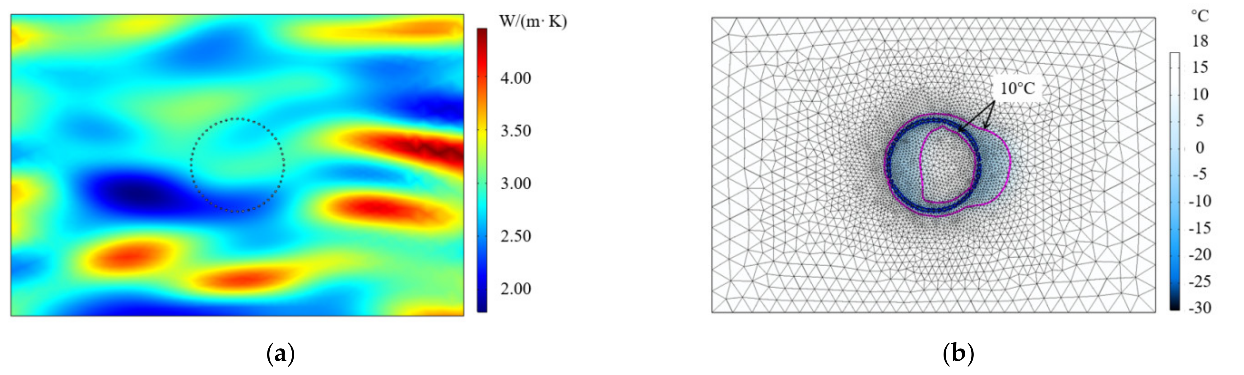
3.3. Random Field of Soil Thermal Conductivity
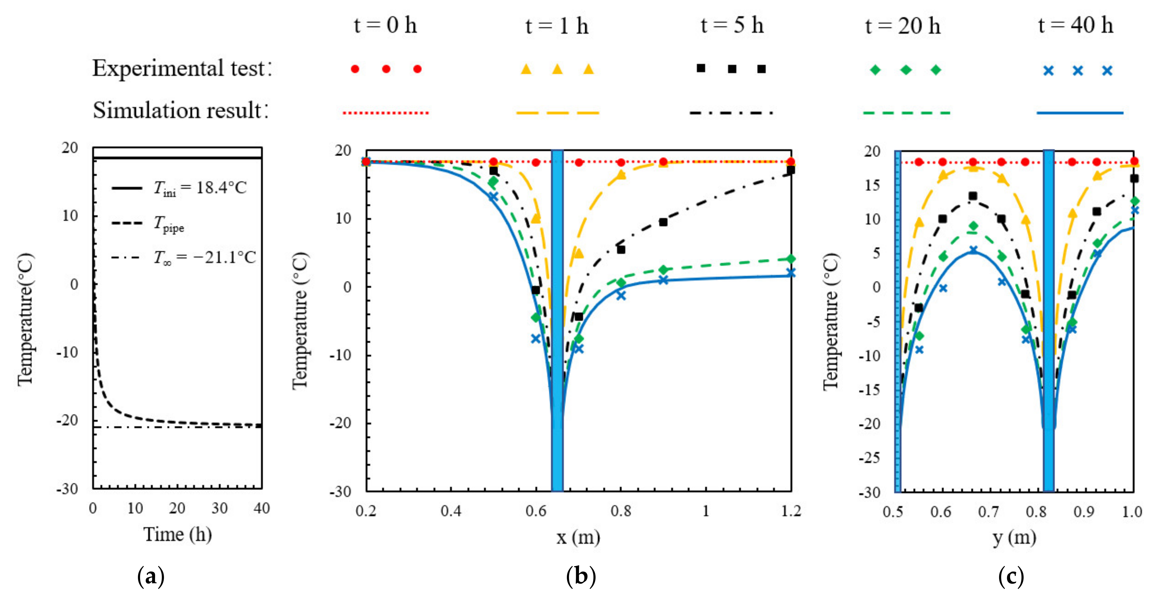
3.4. Model Validation
4. Results and Discussion
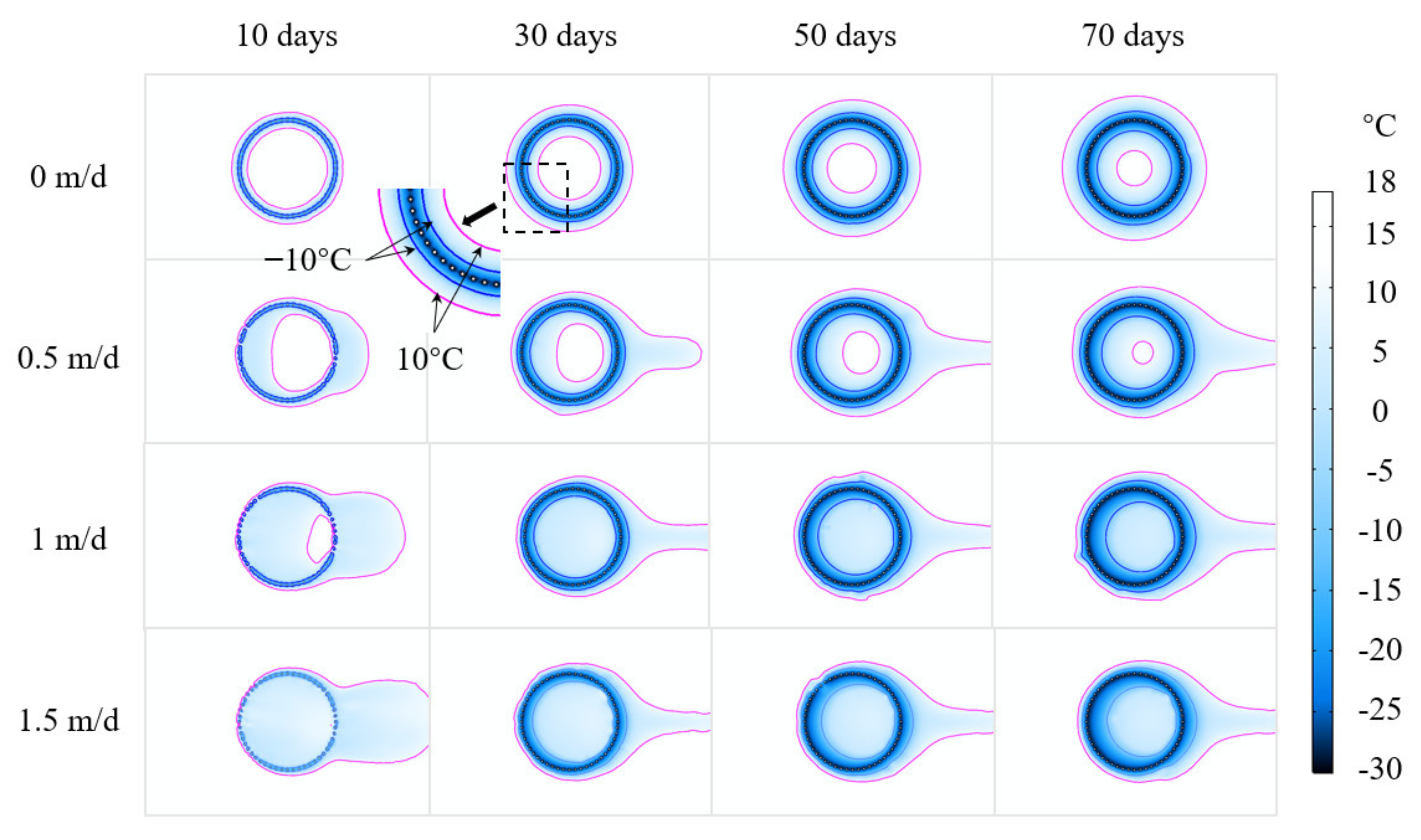
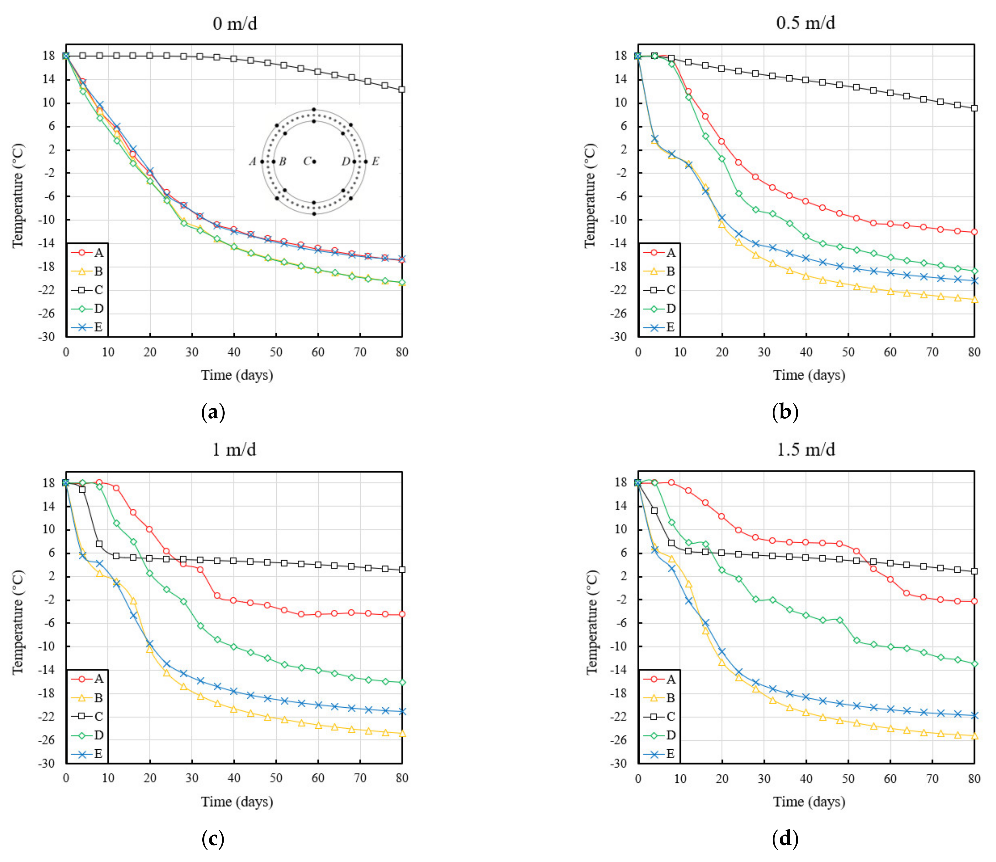
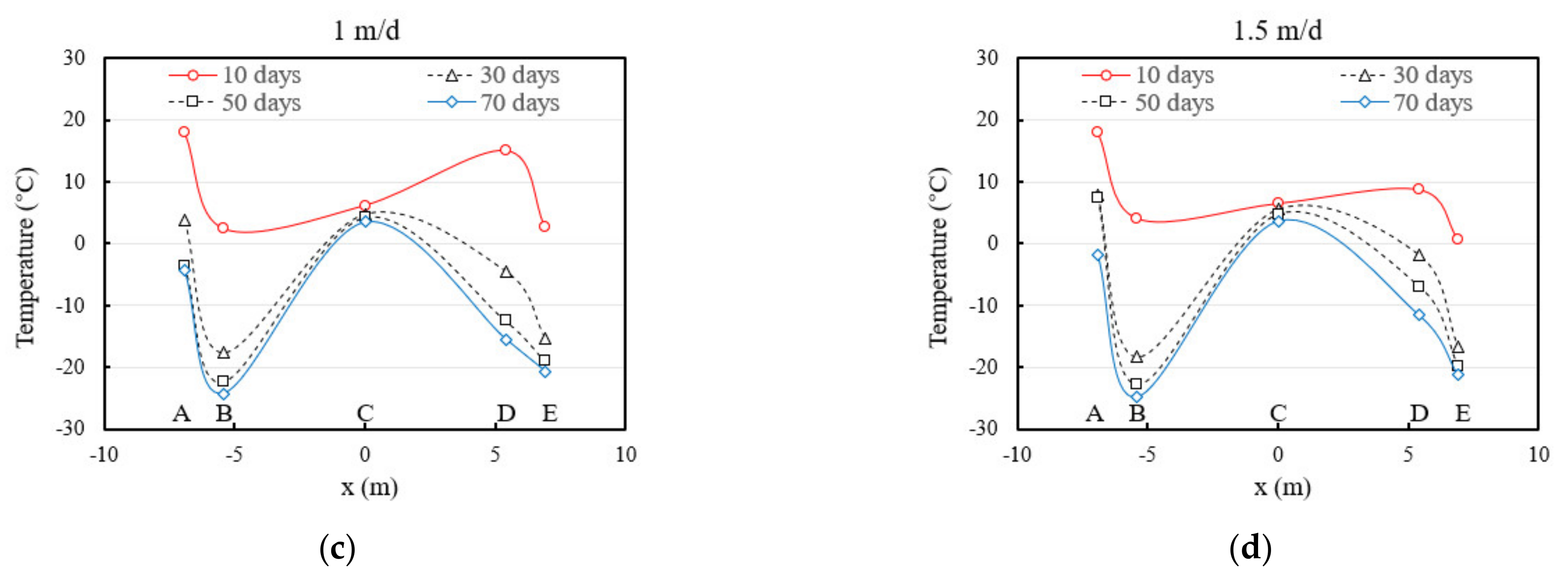
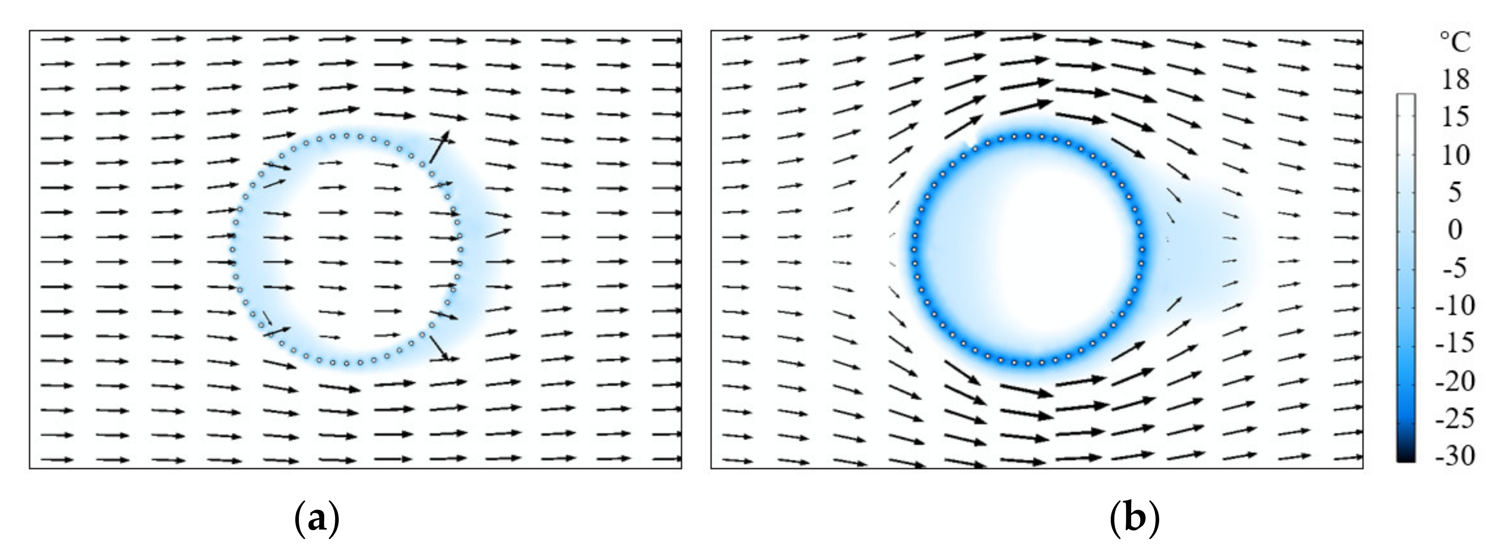
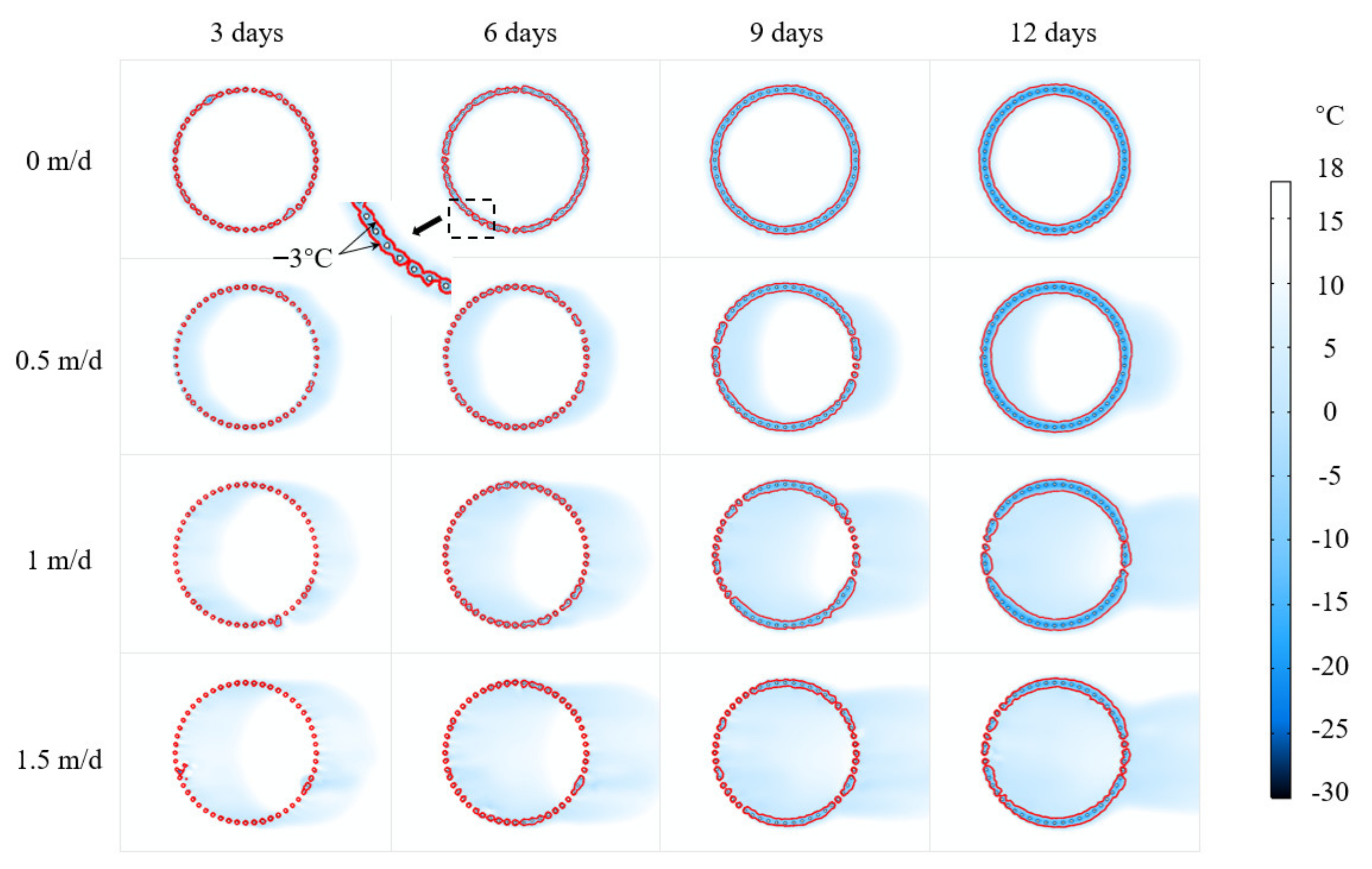
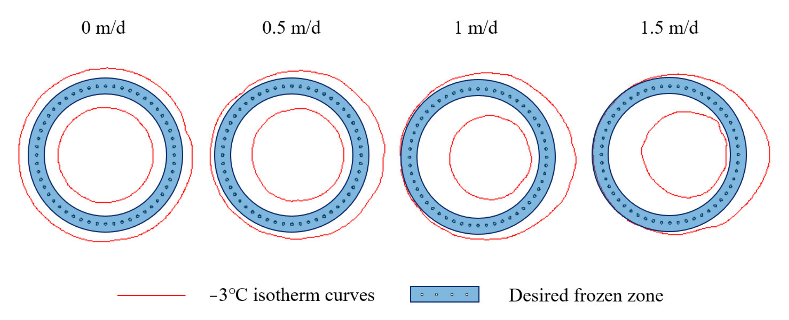
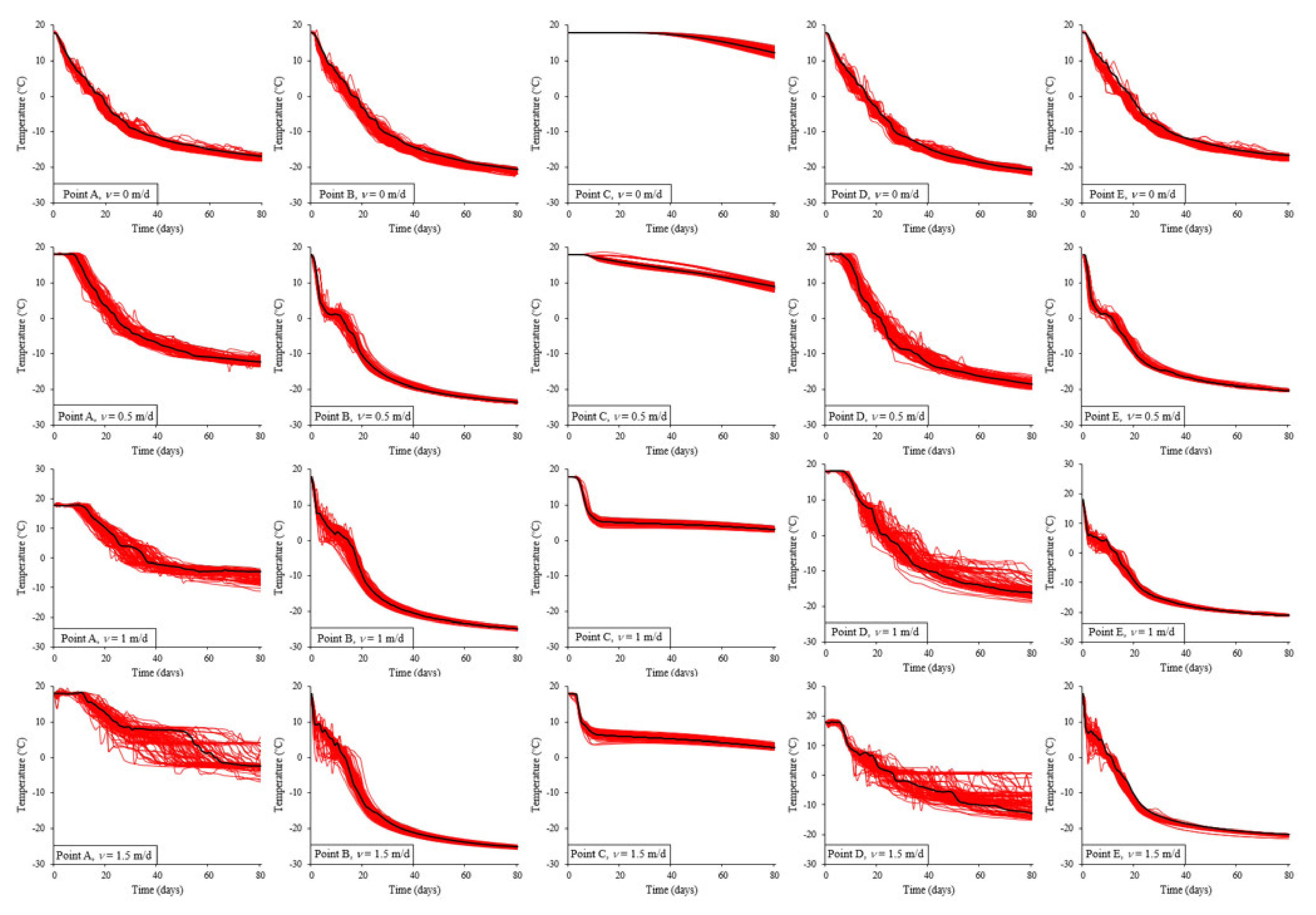
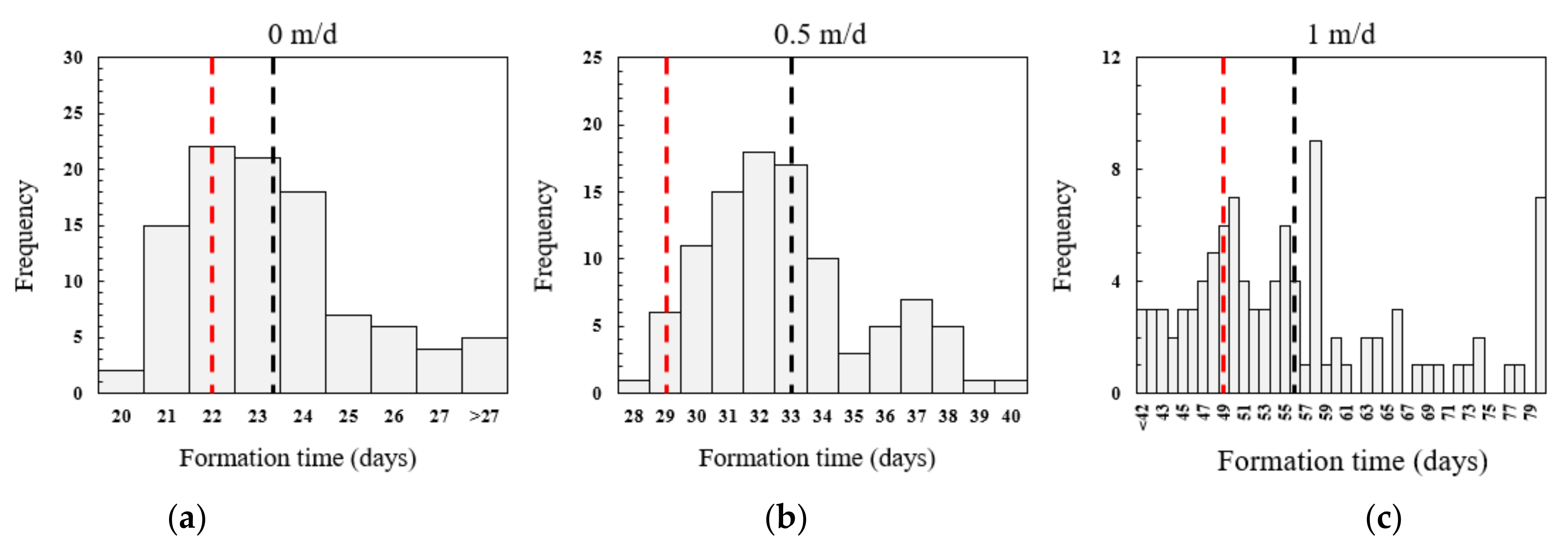
4.1. Effects of Seepage
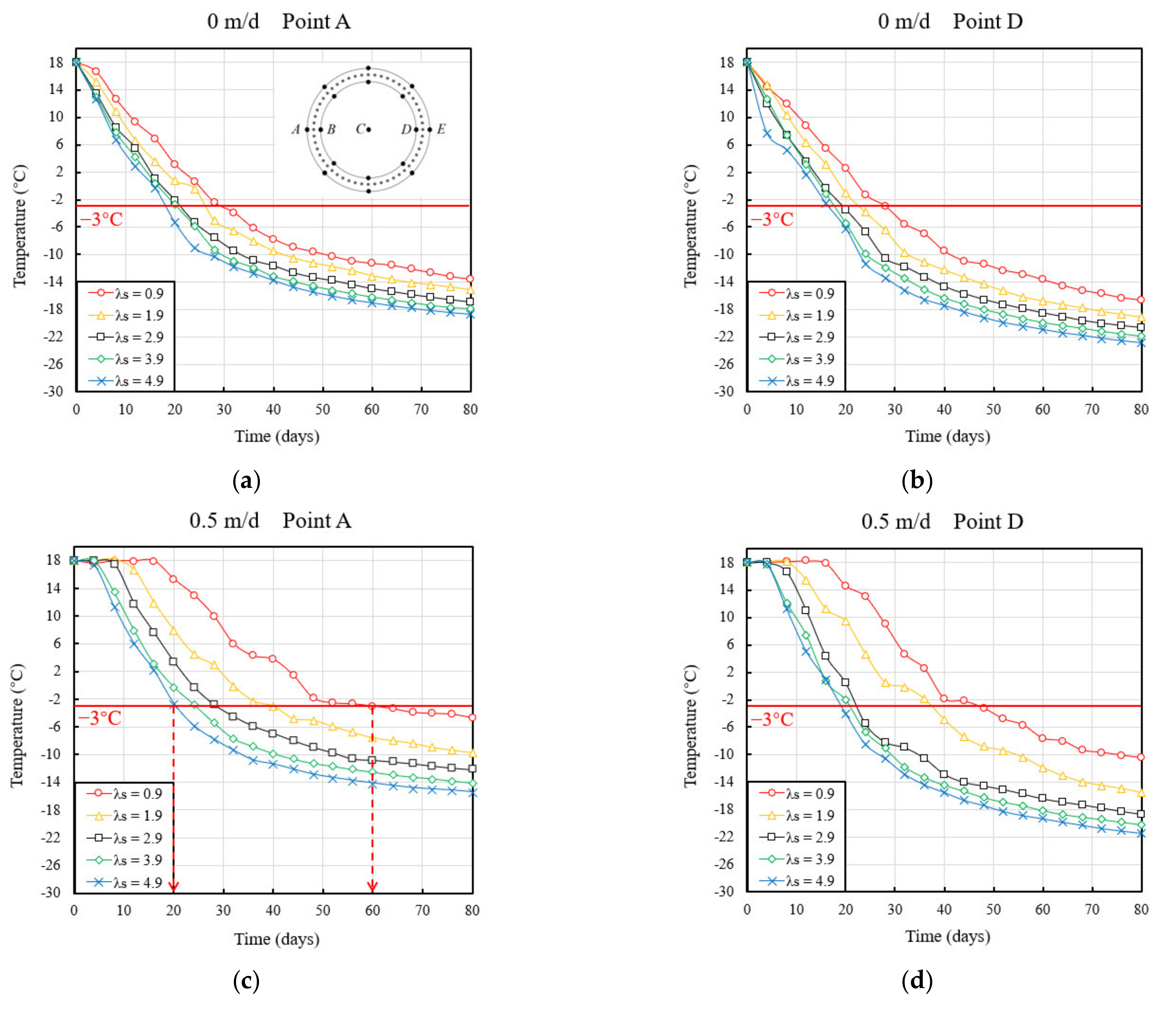
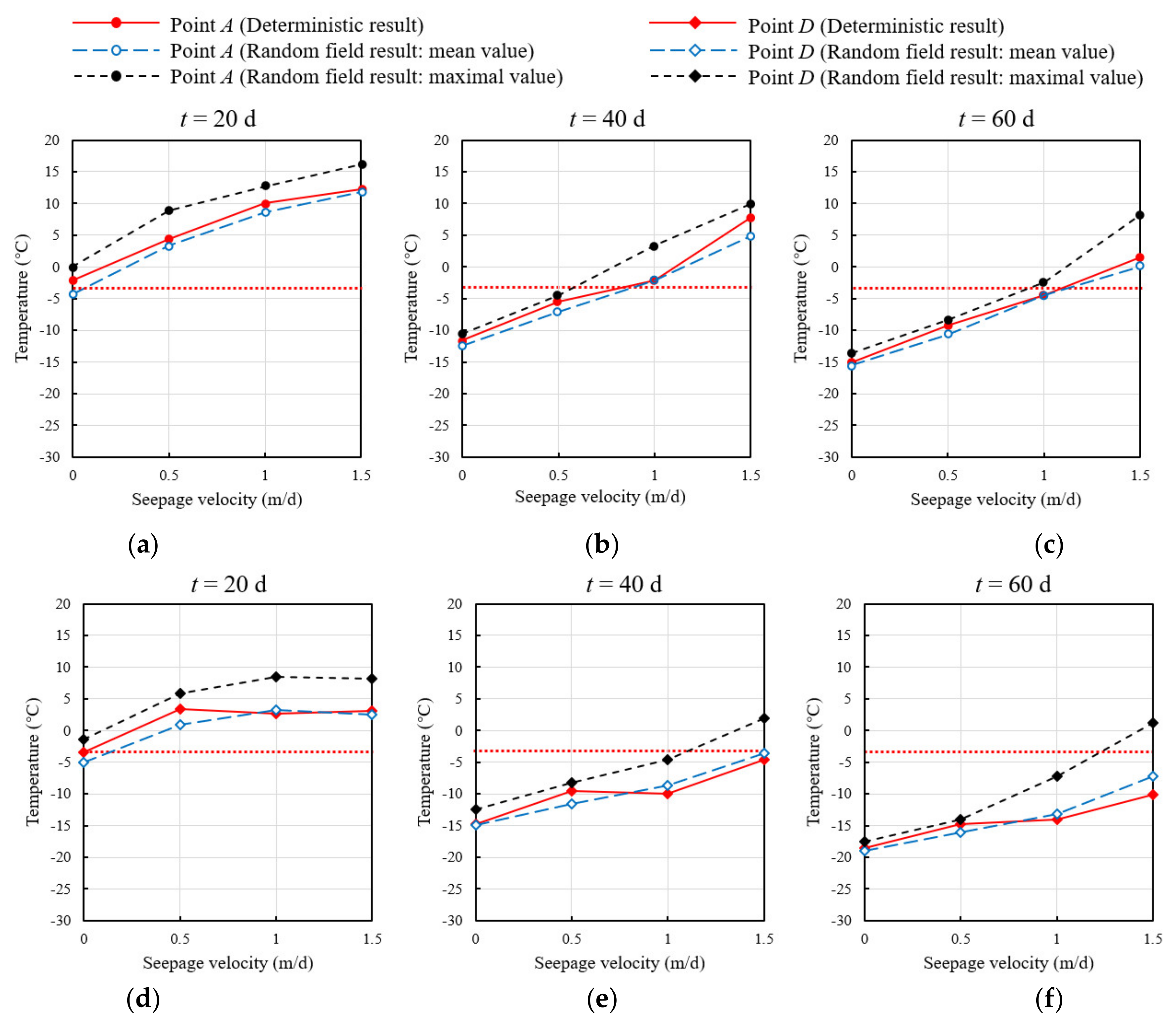
4.2. Effects of Soil Thermal Conductivity
5. Conclusions
Author Contributions
Funding
Institutional Review Board Statement
Informed Consent Statement
Conflicts of Interest
Nomenclature
| Ceq | Equivalent volumetric heat capacity |
| Cf | Volumetric heat capacity in the frozen zone |
| Ci | Heat capacity of ice |
| Cs | Heat capacity of soil solid |
| Cu | Volumetric heat capacity in the unfrozen zone |
| Cw | Heat capacity of water |
| COV | Coefficient of variation |
| d | Diameter of freeze pipe |
| Etot | Total error measure |
| g | Gravity acceleration |
| Gi | Power spectral density function |
| Gj | Power spectral density function |
| Kr | Relative permeability |
| lx | Correlation distance in abscissa direction |
| ly | Correlation distance in ordinate direction |
| Lf | Latent heat |
| m | Material constant |
| n | Porosity |
| N | Order of random number matric |
| P | Fluid pressure |
| q | Conductive heat flux |
| R | Radius of pipe circle |
| R1 | Random number matric |
| R2 | Random number matric |
| t | Time |
| T | Temperature |
| T0 | Freezing point |
| Te | Temperature of experimental test |
| Tini | Initial temperature of soil and seepages |
| Tpipe | Final temperature of freeze pipes |
| Ts | Temperature of simulation result |
| T∞ | Final temperature of freeze pipes |
| w | Material constant |
| z | Material constant |
| λe | Effective thermal conductivity |
| λi | Thermal conductivity of ice |
| λs | Thermal conductivity of soil solid |
| λw | Thermal conductivity of water |
| κ | Intrinsic permeability |
| γ | Unfrozen water content |
| μw | Dynamic viscosity |
| μλs | Mean value of soil thermal conductivity |
| vw | Velocity field of fluid water |
| ρi | Density of ice |
| ρs | Density of soil |
| ρw | Density of water |
| ωi | Frequency coordinate value |
| ωj | Frequency coordinate value |
| Δω | Discrete interval of frequency coordinate |
| σi | Standard deviation |
| σj | Standard deviation |
References
- Pimentel, E.; Papakonstantinou, S.; Anagnostou, G. Numerical interpretation of temperature distributions from three ground freezing applications in urban tunnelling. Tunn. Undergr. Space Technol. 2012, 28, 57–69. [Google Scholar] [CrossRef]
- Kim, Y.S.; Kang, J.M.; Lee, J.; Hong SSKim, K.J. Finite element modeling and analysis for artificial ground freezing in egress shafts. KSCE J. Civ. Eng. 2012, 16, 925–932. [Google Scholar] [CrossRef]
- Vitel, M.; Rouabhi, A.; Tijani, M.; Guérin, F. Modeling heat transfer between a freeze pipe and the surrounding ground during artificial ground freezing activities. Comput. Geotech. 2015, 63, 99–111. [Google Scholar] [CrossRef]
- Ou, C.Y.; Kao, C.C.; Chen, C.I. Performance and analysis of artificial ground freezing in the shield tunneling. J. Geoengin. 2009, 4, 29–40. [Google Scholar] [CrossRef]
- McKenzie, J.M.; Voss, C.I.; Siegel, D.I. Groundwater flow with energy transport and water–ice phase change: Numerical simulations, benchmarks, and application to freezing in peat bogs. Adv. Water Resour. 2007, 30, 966–983. [Google Scholar] [CrossRef]
- Nishimura, S.; Gens, A.; Olivella, S.; Jardine, R.J. THM-coupled finite element analysis of frozen soil: Formulation and application. Géotechnique 2009, 59, 159–171. [Google Scholar] [CrossRef] [Green Version]
- Zhao, X.; Zhou, G.; Wang, J. Deformation and strength behaviors of frozen clay with thermal gradient under uniaxial compression. Tunn. Undergr. Space Technol. 2013, 38, 550–558. [Google Scholar] [CrossRef]
- Xu, X.; Wang, Y.; Bai, R.; Fan, C.; Hua, S. Comparative studies on mechanical behavior of frozen natural saline silty sand and frozen desalted silty sand. Cold Reg. Sci. Technol. 2016, 132, 81–88. [Google Scholar] [CrossRef]
- Liu, Y.; Hu, J.; Xiao, H.; Chen, E.J. Effects of material and drilling uncertainties on artificial ground freezing of cement-admixed soils. Can. Geotech. J. 2017, 54, 1659–1671. [Google Scholar] [CrossRef]
- Liu, Y.; Li, K.-Q.; Li, D.-Q.; Tang, X.-S.; Gu, S.-X. Coupled thermal–hydraulic modeling of artificial ground freezing with uncertainties in pipe inclination and thermal conductivity. Acta Geotech. 2021, 1–18. [Google Scholar] [CrossRef]
- Alzoubi, M.; Nie-Rouquette, A.; Sasmito, A.P. Conjugate heat transfer in artificial ground freezing using enthalpy-porosity method: Experiments and model validation. Int. J. Heat Mass Transf. 2018, 126, 740–752. [Google Scholar] [CrossRef]
- Alzoubi, M.; Madiseh, S.A.G.; Hassani, F.P.; Sasmito, A.P. Heat transfer analysis in artificial ground freezing under high seepage: Validation and heatlines visualization. Int. J. Therm. Sci. 2019, 139, 232–245. [Google Scholar] [CrossRef]
- Zhou, M.; Meschke, G. A three-phase thermo-hydro-mechanical finite element model for freezing soils. Int. J. Numer. Anal. Methods Geéomeéch. 2013, 37, 3173–3193. [Google Scholar] [CrossRef]
- Vitel, M.; Rouabhi, A.; Tijani, M.; Guérin, F. Modeling heat and mass transfer during ground freezing subjected to high seepage velocities. Comput. Geotech. 2016, 73, 1–15. [Google Scholar] [CrossRef]
- Marwan, A.; Zhou, M.-M.; Abdelrehim, M.Z.; Meschke, G. Optimization of artificial ground freezing in tunneling in the presence of seepage flow. Comput. Geotech. 2016, 75, 112–125. [Google Scholar] [CrossRef]
- Huang, S.; Guo, Y.; Liu, Y.; Ke, L.; Liu, G.; Chen, C. Study on the influence of water flow on temperature around freeze pipes and its distribution optimization during artificial ground freezing. Appl. Therm. Eng. 2018, 135, 435–445. [Google Scholar] [CrossRef]
- Papakonstantinou, S.; Anagnostou, G.; Pimentel, E. Evaluation of ground freezing data from the Naples subway. Proc. Inst. Civ. Eng. Geotech. Eng. 2013, 166, 280–298. [Google Scholar] [CrossRef]
- Semin, M.A.; Levin, L.Y.; Pugin, A.V. Analysis of Earth’s Heat Flow in Artificial Ground Freezing. J. Min. Sci. 2020, 56, 149–158. [Google Scholar] [CrossRef]
- Goh, A.; Zhang, W.; Wong, K. Deterministic and reliability analysis of basal heave stability for excavation in spatial variable soils. Comput. Geotech. 2019, 108, 152–160. [Google Scholar] [CrossRef]
- Liu, Y.; He, L.Q.; Jiang, Y.J.; Sun, M.M.; Chen, E.J.; Lee, F.-H. Effect of in situ water content variation on the spatial variation of strength of deep cement-mixed clay. Géotechnique 2019, 69, 391–405. [Google Scholar] [CrossRef] [Green Version]
- Luo, Z.; Hu, B.; Wang, Y.; Di, H. Effect of spatial variability of soft clays on geotechnical design of braced excavations: A case study of Formosa excavation. Comput. Geotech. 2018, 103, 242–253. [Google Scholar] [CrossRef]
- Pan, Y.; Shi, G.; Liu, Y.; Lee, F.H. Effect of spatial variability on performance of cement-treated soil slab during deep excavation. Constr. Build. Mater. 2018, 188, 505–519. [Google Scholar] [CrossRef]
- Pan, Y.; Liu, Y.; Xiao, H.; Lee, F.H.; Phoon, K.K. Effect of spatial variability on short-and long-term behaviour of axially-loaded cement-admixed marine clay column. Comput. Geotech. 2018, 94, 150–168. [Google Scholar] [CrossRef]
- El Haj, A.K.; Soubra, A.H.; Fajoui, J. Probabilistic analysis of an offshore monopile foundation taking into account the soil spatial variability. Comput. Geotech. 2019, 106, 205–216. [Google Scholar] [CrossRef]
- Gholampour, A.; Johari, A. Reliability-based analysis of braced excavation in unsaturated soils considering conditional spatial variability. Comput. Geotech. 2019, 115, 103163. [Google Scholar] [CrossRef]
- Liu, Y.; Lee, F.H.; Quek, S.T.; Chen, E.J.; Yi, J.T. Effect of spatial variation of strength and modulus on the lateral compression response of cement-admixed clay slab. Géotechnique 2015, 65, 851–865. [Google Scholar] [CrossRef]
- Luo, Z.; Hu, B. Probabilistic design model for energy piles considering soil spatial variability. Comput. Geotech. 2019, 108, 308–318. [Google Scholar] [CrossRef]
- Pan, Y.; Liu, Y.; Chen, E.J. Probabilistic investigation on defective jet-grouted cut-off wall with random geometric imperfections. Géotechnique 2019, 69, 420–433. [Google Scholar] [CrossRef]
- Wang, T.; Zhou, G.; Wang, J.; Zhou, L. Stochastic analysis of uncertain thermal parameters for random thermal regime of frozen soil around a single freeze pipe. Heat Mass Transf. 2018, 54, 2845–2852. [Google Scholar] [CrossRef]
- Cai, H.; Li, S.; Liang, Y.; Yao, Z.; Cheng, H. Model test and numerical simulation of frost heave during twin-tunnel construction using artificial ground-freezing technique. Comput. Geotech. 2019, 115, 103155. [Google Scholar] [CrossRef]
- Tang, Y.; Xiao, S.; Zhou, J. Deformation prediction and deformation characteristics of multilayers of mucky clay under artificial freezing condition. KSCE J. Civ. Eng. 2019, 23, 1064–1076. [Google Scholar] [CrossRef]
- Tan, X.; Chen, W.; Tian, H.; Cao, J. Water flow and heat transport including ice/water phase change in porous media: Numerical simulation and application. Cold Reg. Sci. Technol. 2011, 68, 74–84. [Google Scholar] [CrossRef]
- Panteleev, I.; Kostina, A.; Zhelnin, M.; Plekhov, A.; Levin, L. Intellectual monitoring of artificial ground freezing in the fluid-saturated rock mass. Proc. Struct. Integr. 2017, 5, 492–499. [Google Scholar] [CrossRef]
- Amiri, E.A.; Craig, J.R.; Kurylyk, B.L. A theoretical extension of the soil freezing curve paradigm. Adv. Water Resour. 2018, 111, 319–328. [Google Scholar] [CrossRef]
- Grenier, C.; Anbergen, H.; Bense, V.; Chanzy, Q.; Coon, E.; Collier, N.; Voss, C. Groundwater flow and heat transport for systems undergoing freeze-thaw: Intercomparison of numerical simulators for 2D test cases. Adv. Water Resour. 2018, 114, 196–218. [Google Scholar] [CrossRef]
- Lide, D.R. Handbook of Chemistry and Physics, 84th ed.; CRC Press: Boca Raton, FL, USA, 2003; pp. 980–981. [Google Scholar]
- Vitel, M.; Rouabhi, A.; Tijani, M.; Guérin, F. Thermo-hydraulic modeling of artificial ground freezing: Application to an underground mine in fractured sandstone. Comput. Geotech. 2016, 75, 80–92. [Google Scholar] [CrossRef]
- Hu, J.; Liu, Y.; Wei, H.; Yao, K.; Wang, W. Finite-element analysis of heat transfer of horizontal ground-freezing method in shield-driven tunneling. Int. J. Geomech. 2017, 17, 04017080. [Google Scholar] [CrossRef]
- Hu, X.D.; Deng, S.J. Ground freezing application of intake installing construction of an underwater tunnel. Proc. Eng. 2016, 165, 633–640. [Google Scholar] [CrossRef]
- Shinozuka, M.; Deodatis, G. Simulation of the stochastic process by spectral representation. Appl. Mech. Rev. 1991, 44, 191–204. [Google Scholar] [CrossRef]
- Shinozuka, M.; Deodatis, G. Simulation of multi-dimensional Gaussian stochastic fields by spectral representation. Appl. Mech. Rev. 1996, 49, 29–53. [Google Scholar] [CrossRef]
- Pimentel, E.; Sres, A.; Anagnostou, G. Large-scale laboratory tests on artificial ground freezing under seepage-flow conditions. Géotechnique 2012, 62, 227–241. [Google Scholar] [CrossRef]
- Yamamoto, Y.; Springman, S.M. Axial compression stress path tests on artificial frozen soil samples in a triaxial device at temperatures just below 0 °C. Can. Geotech. J. 2014, 51, 1178–1195. [Google Scholar] [CrossRef]
- Locatelli, L.; Binning, P.J.; Sanchez-Vila, X.; Søndergaard, G.L.; Rosenberg, L.; Bjerg, P.L. A simple contaminant fate and transport modelling tool for management and risk assessment of groundwater pollution from contaminated sites. J. Contam. Hydrol. 2019, 221, 35–49. [Google Scholar] [CrossRef] [PubMed]


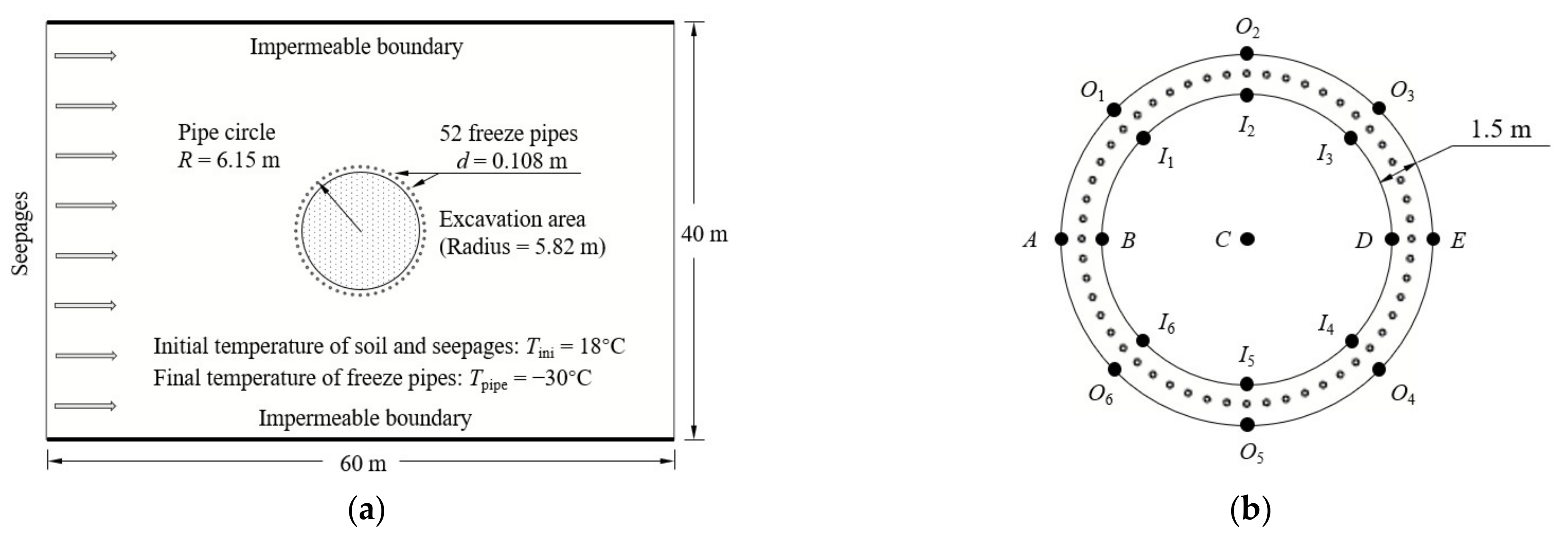
| Point No. | Coordinate (m) | |
|---|---|---|
| x (Horizontal) | y (Vertical) | |
| A | −6.9 | 0 |
| B | −5.4 | 0 |
| C (Origin) | 0 | 0 |
| D | 5.4 | 0 |
| E | 6.9 | 0 |
| O1 | −4.88 | 4.88 |
| I1 | −3.82 | 3.82 |
| O2 | 0 | 6.9 |
| I2 | 0 | 5.4 |
| O3 | 4.88 | 4.88 |
| I3 | 3.82 | 3.82 |
| O4 | 4.88 | −4.88 |
| I4 | 3.82 | −3.82 |
| O5 | 0 | −6.9 |
| I5 | 0 | −5.4 |
| O6 | −4.88 | −4.88 |
| I6 | −3.82 | −3.82 |
| Description | Symbol | Value | Unit |
|---|---|---|---|
| Density of soil | ρs | 1900 | kg·m−3 |
| Density of water | ρw | 1000 | kg·m−3 |
| Density of ice | ρi | 910 | kg·m−3 |
| Thermal conductivity of soil solid | λs | 2.9 | W·m−1 K−1 |
| Thermal conductivity of water | λw | 0.6 | W·m−1 K−1 |
| Thermal conductivity of ice | λi | 2.4 | W·m−1 K−1 |
| Heat capacity of soil solid | Cs | 1300 | J·kg−1 K−1 |
| Heat capacity of water | Cw | 4200 | J·kg−1 K−1 |
| Heat capacity of ice | Ci | 2100 | J·kg−1 K−1 |
| Material constant | m | 0.7 | / |
| Porosity | n | 0.4 | / |
| Material constant | w | 0.5 | °C |
| Material constant | z | 0.7 | / |
| Intrinsic permeability | κ | 1 × 10⁻¹¹ | m2 |
| Dynamic viscosity (at Tini) | μw | 0.001 | Pa·s |
| Freezing point | T0 | 0 | °C |
| Initial temperature | Tini | 18 | °C |
| Latent heat | Lf | 334 | kJ·kg−1 |
| Gravity acceleration | g | 9.8 | m·s−2 |
| Time (Day) | 0 | 1 | 5 | 10 | 15 | 20 | 40 | 80 |
|---|---|---|---|---|---|---|---|---|
| Temperature (°C) | 18 | 0 | −10 | −20 | −25 | −30 | −30 | −30 |
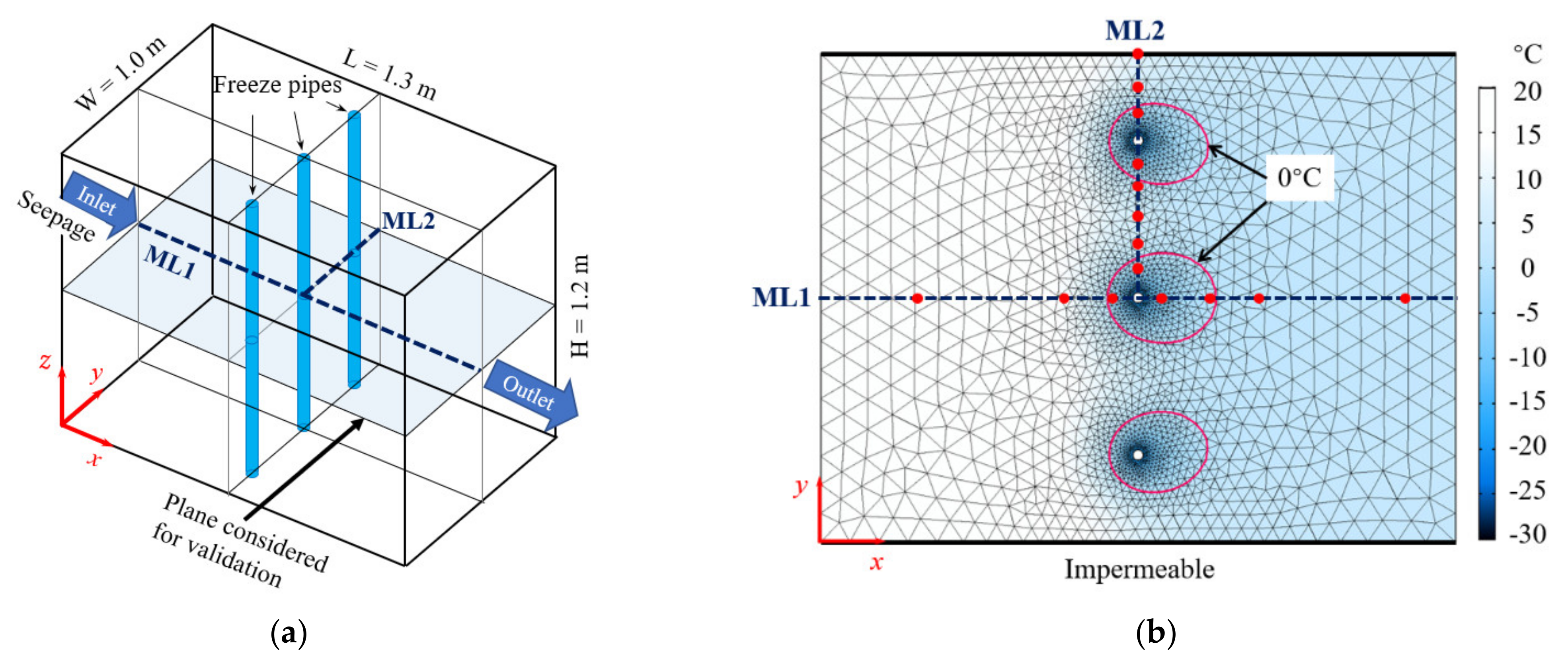
| Typical Duration | 0 h | 1 h | 5 h | 20 h | 40 h |
|---|---|---|---|---|---|
| Etot along ML1 (%) | 0.87 | 6.59 | 14.9 | 15.58 | 19.85 |
| Etot along ML2 (%) | 0.59 | 2.75 | 21.21 | 29.18 | 37.32 |
| Point | Seepage Velocity (m/d) | Deterministic Value (°C) | Average (°C) | Standard Deviation (°C) | Range (°C) |
|---|---|---|---|---|---|
| A | 0 | −16.93 | −17.17 | 0.55 | 2.36 |
| 0.5 | −12.15 | −12.14 | 0.76 | 3.39 | |
| 1 | −4.54 | −5.58 | 1.65 | 7.49 | |
| 1.5 | −2.33 | −2.07 | 2.17 | 12.61 | |
| B | 0 | −20.65 | −21.09 | 0.41 | 1.89 |
| 0.5 | −23.59 | −23.52 | 0.26 | 1.21 | |
| 1 | −24.85 | −24.76 | 0.25 | 1.17 | |
| 1.5 | −25.22 | −25.27 | 0.24 | 1.26 | |
| C | 0 | 12.2 | 12.27 | 0.83 | 3.03 |
| 0.5 | 9 | 8.96 | 0.62 | 2.9 | |
| 1 | 3.07 | 3.08 | 0.39 | 1.84 | |
| 1.5 | 2.85 | 3.09 | 0.47 | 2.04 | |
| D | 0 | −20.72 | −21.07 | 0.49 | 2.25 |
| 0.5 | −18.69 | −18.52 | 0.78 | 3.98 | |
| 1 | −16.12 | −15.9 | 1.69 | 8.92 | |
| 1.5 | −12.87 | −10.31 | 3.44 | 15.92 | |
| E | 0 | −16.73 | −17.27 | 0.53 | 2.16 |
| 0.5 | −20.37 | −20.3 | 0.22 | 1.83 | |
| 1 | −21.09 | −21.15 | 0.18 | 0.84 | |
| 1.5 | −21.71 | −21.89 | 0.22 | 1.35 |
Publisher’s Note: MDPI stays neutral with regard to jurisdictional claims in published maps and institutional affiliations. |
© 2021 by the authors. Licensee MDPI, Basel, Switzerland. This article is an open access article distributed under the terms and conditions of the Creative Commons Attribution (CC BY) license (https://creativecommons.org/licenses/by/4.0/).
Share and Cite
Qiu, P.; Li, P.; Hu, J.; Liu, Y. Modeling Seepage Flow and Spatial Variability of Soil Thermal Conductivity during Artificial Ground Freezing for Tunnel Excavation. Appl. Sci. 2021, 11, 6275. https://doi.org/10.3390/app11146275
Qiu P, Li P, Hu J, Liu Y. Modeling Seepage Flow and Spatial Variability of Soil Thermal Conductivity during Artificial Ground Freezing for Tunnel Excavation. Applied Sciences. 2021; 11(14):6275. https://doi.org/10.3390/app11146275
Chicago/Turabian StyleQiu, Pu, Peitao Li, Jun Hu, and Yong Liu. 2021. "Modeling Seepage Flow and Spatial Variability of Soil Thermal Conductivity during Artificial Ground Freezing for Tunnel Excavation" Applied Sciences 11, no. 14: 6275. https://doi.org/10.3390/app11146275
APA StyleQiu, P., Li, P., Hu, J., & Liu, Y. (2021). Modeling Seepage Flow and Spatial Variability of Soil Thermal Conductivity during Artificial Ground Freezing for Tunnel Excavation. Applied Sciences, 11(14), 6275. https://doi.org/10.3390/app11146275