Data-Driven Approach for Rainfall-Runoff Modelling Using Equilibrium Optimizer Coupled Extreme Learning Machine and Deep Neural Network

Abstract

Rainfall-runoff (R-R) modelling is used to study the runoff generation of a catchment. The quantity or rate of change measure of the hydrological variable, called runoff, is important for environmental scientists to accomplish water-related planning and design. This paper proposes (i) an integrated model namely EO-ELM (an integration of equilibrium optimizer (EO) and extreme learning machine (ELM)) and (ii) a deep neural network (DNN) for one day-ahead R-R modelling. The proposed R-R models are validated at two different benchmark stations of the catchments, namely river Teifi at Glanteifi and river Fal at Tregony in the UK. Firstly, a partial autocorrelation function (PACF) is used for optimal number of lag inputs to deploy the proposed models. Six other well-known machine learning models, called ELM, kernel ELM (KELM), and particle swarm optimization-based ELM (PSO-ELM), support vector regression (SVR), artificial neural network (ANN) and gradient boosting machine (GBM) are utilized to validate the two proposed models in terms of prediction efficiency. Furthermore, to increase the performance of the proposed models, paper utilizes a discrete wavelet-based data pre-processing technique is applied in rainfall and runoff data. The performance of wavelet-based EO-ELM and DNN are compared with wavelet-based ELM (WELM), KELM (WKELM), PSO-ELM (WPSO-ELM), SVR (WSVR), ANN (WANN) and GBM (WGBM). An uncertainty analysis and two-tailed t-test are carried out to ensure the trustworthiness and efficacy of the proposed models. The experimental results for two different time series datasets show that the EO-ELM performs better in an optimal number of lags than the others. In the case of wavelet-based daily R-R modelling, proposed models performed better and showed robustness compared to other models used. Therefore, this paper shows the efficient applicability of EO-ELM and DNN in R-R modelling that may be used in the hydrological modelling field.

1. Introduction

The rainfall-runoff (R-R) modelling process is conducted by hydrologists for forecasting hydrological information (discharge data) which may be helpful in water resources engineering [1,2], flood mitigation planning [3], production of hydroelectric power [4], reservoir operation planning [5]. Additionally, river discharge forecasting information supports the design of dams or water-related infrastructure [3] and the prediction of disasters related to water [6]. Therefore, it is necessary to develop new models along with improving the existing ones to understand the regional and local changes in streamflow for ungauged basins [7] and support the aforementioned issues [8,9].

The R-R process is very complicated due to the complex interaction of several environmental spatio-temporal factors and their effects [10,11,12]. In the R-R process, precipitation is distributed over a catchment and transformed into channel flow or streamflow of river comprises many interacting processes upon the Earth’s surface. These interactions occur in several spatial and temporal scales. This is happening because of diverse characteristics and non-uniformity in the medium of water flow. The hydrological cycle interacts with other disciplines such as ecology, atmospheric science, geology, and mainly with agronomy and land-use management shows diversity of these medium. Therefore, most of the catchment system is highly dynamic and non-linear in nature. It is difficult to provide an effective system which simulates these complex natures. It is also difficult to collect more predictor variables with large samples from a catchment system. The main challenges in R-R modeling comes from the integration of complexities within a catchment system and the difficulty of precise and quantitative representation of available information. In general, the hydrological models can be defined by two groups: (i) physically based and conceptual models, (ii) empirical or data-driven models. The former models require a large number of input parameters, a great amount of hydro-meteorological dataset and precise simulation of nature’s law for hydrological modeling such as R-R modeling. These requirements for the first group of models often limit their usability to model hydrological processes [13]. The data-driven models forecast time series data of hydrological ones using only lag information of time series observations of predictors. These models are broadly used in R-R modeling and do not require large dataset with more predictors and physical laws of nature [14,15].

In recent studies, it was observed that the classical models like auto-regressive integrated moving average (ARIMA) may not be able to simulate the R-R process effectively due to its complex and non-linear nature. A typical data-driven model called single hidden layer feed-forward neural networks (SLFNs) has been broadly used in hydrological time series modeling [16,17,18]. However, the gradient-based learning parameter calibration in SLFNs may suffer from a local convergence problem, long training time and overfitting problem. The use of metaheuristic-based optimization approaches may provide a more generalized network [19,20]. In recent machine learning model development, for significant enhancement of SLFNs, a novel approach called extreme learning machine (ELM) was proposed [21]. With faster learning capability, ELM provides good generalization ability in SLFNs compared to gradient-based SLFNs. This promotes the applicability of ELM in hydro-environmental modeling like streamflow forecasting [22,23], temperature prediction [24], drought index forecasting [25], water quality parameter modeling [26], etc. However, the daily R-R modeling depends on generated rainfall and runoff data which are highly non-linear in nature and time-dependent. In forecasting runoff value, ELM may fall into the local optimum for the stochastic/random selection of input weights and hidden biases [27]. Therefore, effective methods are required to improve the ELM performance for daily R-R modeling [28,29]. In recent years, evolutionary algorithms have been widely used to train neural networks because of their better global searching ability that enhances the model performance [30,31,32,33]. For example, particle swarm optimization (PSO), biogeography-based optimization (BBO) and grey wolf optimization (GWO) were used to enhance the performance of ELM models in several engineering applications [34,35,36,37,38].

Recently, Faramarzi et al. [39] proposed a novel optimization algorithm called equilibrium optimizer (EO), inspired by accounting mass balance mathematical equations within a control volume. The mass balance equations are based on the conservation of mass law in physics. The mass balance equations estimate the dynamic and equilibrium state of object of interest within a defined system boundary. EO has several dominance properties for qualifying a good optimization algorithm. It is easy to implement, proposes good balance between exploration and exploitation tasks and population diversity in individuals. Therefore, it may be used to solve various optimization problems. This study integrated EO with ELM and validated it by R-R modelling.

On the other hand, deep neural networks (DNNs) are successfully used for solving complex problems using high-dimensional data [40]. DNN approach has been successfully applied in fields like natural language processing [41], speech recognition [42], bioinformatics [43] and image recognition [44]. Deep learning has shown promise for modeling time-series data through techniques like Conditional RBM (restricted Boltzmann machine), RBM, recurrent neural network (RNN), and auto encoder [45]. In this study, a multiple layer of neural network, called DNN model, is developed for R-R modelling.

This paper proposes EO-based optimization of ELM learning parameters (EO-ELM) to avoid a trap into local optima and enhance the generalization capability of the network and a DNN model for R-R modelling. The two different benchmark stations of the catchments in the United Kingdom (UK) are used to validate the performance efficacy of the proposed models. The catchments were the river Teifi at Glanteifi and the river Fal at Tregony. The river gauges of the two catchments were from the UK benchmark network stations and were suitable for high, low, and medium flow analysis [46]. The predictors are daily rainfall and runoff time series datasets. The preceding days of rainfall and runoff were selected as the input features for the ML models. A partial autocorrelation function (PACF) was used for optimal number of correlated preceding days. Furthermore, the performance of the proposed models was compared with the performance of other well-known models, called ELM, kernel (radial basis function (RBF)) ELM (KELM), PSO optimized ELM (PSO-ELM), support vector regression (SVR), artificial neural network (ANN) and gradient boosting machine (GBM)

Furthermore, to enhance prediction accuracy of the proposed models, discrete wavelet transform (DWT)-based pre-processed rainfall and runoff time series data have been used in this study. Recently, DWT-based time series forecasting has been used in several engineering fields to enhance the prediction performance of several machine learning models [47,48,49,50,51,52,53,54,55,56]. All of the previous studies have proved that wavelet-based hybrid models performed with better efficacy compared to single models. Therefore, the paper proposes hybrid wavelet-based R-R models, namely hybrid DWT-based EO-ELM (WEO-ELM) and DWT-based DNN. The performance of WEO-ELM and WDNN is compared with DWT-based ELM (WELM), DWT-based KELM (WKELM), DWT-based hybrid PSO-ELM (WPSO-ELM), DWT-based support vector regression (WSVR), DWT-based artificial neural network (WANN) and DWT-based gradient boosting machine (WGBM) using two-time series datasets.

2. Background of Soft Computing Methods

2.1. Particle Swarm Optimization

Particle swarm optimization (PSO) is a stochastic optimization technique based on a population which is proposed by Russell Eberhart and James Kennedy in 1995, inspired by social behavior of the bird flocking or fish schooling [57]. It mimics the navigation and foraging of a flock of birds or school of fishes. PSO uses the number of particles (individuals) moving around the problem space to find the best solution in their path over the course of runs. In other words, PSO has group of particles that move around the problem space. Particles are influenced by their own best past position and the best past position of the whole population (neighbor). These concepts have been mathematically modelled using Equations (1) and (2).

$$v_{i,n}^{j+1}=w{v}_{i,n}^j+c_1{r}_1\left(p_{i,n}^j-x_{i,n}^j\right)+c_2{r}_2\left(p_{g,n}^j-x_{i,n}^j\right)$$

(1)

$$x_{i,n}^{j+1}=x_{i,n}^j+v_{i,n}^{j+1}$$

(2)

where, $v_{i,n}^{j+1}$ indicates new velocity for the i^th particle, c₁ and c₂ specifies weighting coefficients for local best and global best locations respectively, $x_{i,n}^{j+1}$ indicates a particle’s new position. $p_{i,n}^j$ is the i^th particle’s best-known position, and $p_{g,n}^j$ indicates the best position known to the whole swarm, r₁ and r₂ are the uniform random number distribution range between 0 and 1. The authors of this paper utilize PSO to find optimal values of the ELM learning parameters in the training phase.

2.2. Equilibrium Optimizer (EO)

The underlying nature of EO is based on the law of conservation of mass, where mass changing in time is equivalent to the amount of mass entering into a system plus the generated amount of mass inside the system minus the amount of mass leaving that system. More details about the inspiration of EO are given in [39]. Like other population-based optimization techniques, EO has a number of particles (population) as candidate solution and particle’s position is termed as concentration. Each particle’s fitness function is evaluated to determine the equilibrium states of populations for the selection of best solution. The following are the steps of EO:

Step 1: Initialization of particle’s concentrations

The concentrations are initialized randomly for each particle using the upper bound and lower bound of the decision variable which is formulated as:

$$C_i^{init}=C_{lower\_bound}+ran{d}_i\times \left(C_{upper\_bound}-C_{lower\_bound}\right),i=1,2,\dots ,N$$

(3)

where $C_i^{init}$ is $i^{\mathrm{th}}$ particle’s initial concentrations, $C_{upper\_bound}$ and $C_{lower\_bound}$ are the of concentrations upper bound and lower bound respectively, rand_i is the generated random number between 0 and 1, and N is the population size.

Step 2: Candidate solutions in equilibrium pool $\left({\overrightarrow{P}}_{eq, pool}\right)$

The equilibrium pool is a collection of best candidate solutions which consists of five types of global optimal candidates. In the initial optimization period, the positions of the equilibrium candidates are unknown, which are determined in each run of the main loop to provide the knowledge about the search pattern. Among the five global optimum solutions, the four best equilibrium candidates are selected in each run with another one which is an arithmetic mean of four best solutions. The four best solutions are useful for the exploration task and the average one helps in the exploitation phase of the EO algorithm. The number of candidate solutions in equilibrium pool may depend on the nature of the evaluated function. In this work, the authors choose five equilibrium candidates for the problem space. The following is the equilibrium pool:

$${\overrightarrow{P}}_{eq, pool}=\left\{{\overrightarrow{P}}_{eq\left[1\right]}+{\overrightarrow{P}}_{eq\left[2\right]}+{\overrightarrow{P}}_{eq\left[3\right]}+{\overrightarrow{P}}_{eq\left[4\right]}+{\overrightarrow{P}}_{eq\left[mean\right]}\right\}$$

(4)

Particles are randomly selected to update their concentrations with the same probability. During this optimization process all particles receive approximately the same number of updating processes.

Step 3: particle’s concentration updating process

After random selection of particle, the first term is the main concentration updating formula (Equation (5)) called exponential term (F).

$$\overrightarrow{F}=e^{-\overrightarrow{\lambda }\left(t-t_0\right)}$$

(5)

where λ is the turnover rate, i.e., rate of change in concentration within a control volume, which is varying with time and defined as a random vector in between 0 and 1. Variable t (time) is a function of iteration and which has decreasing pattern in each iteration (Equation (6)).

$$t={\left(1-\frac{Iteration}{Max\_iteration}\right)}^{\left(a_2\times \frac{Iteration}{Max\_iteration}\right)}$$

(6)

where Iteration and Max_iteration are the present value and maximum value of iteration, respectively and a₂ is used to control the exploitation task which is a manually specified constant value. To guarantee convergence and balance in between intensification and diversification, t₀ is considered as:

$$t_0=\frac{1}{\overrightarrow{\lambda }}\times \ln \left(-a_1\ast sign\left(\overrightarrow{r}-0.5\right)\left[1-e^{-\overrightarrow{\lambda }t}\right]\right)+t$$

(7)

where a₁ is used to control the exploration task which is a manually specified constant value. The higher value of a₁ means good exploration ability and lower exploitation efficiency. Equally, the higher value of a₂ means good exploitation ability and lower exploration efficiency. $sign\left(\overrightarrow{r}-0.5\right)$ component specifies the direction of intensification and diversification of particles and r is defined as a random vector in between 0 and 1.

The final equation of F is defined by substituting Equation (5) with Equation (7) as follows:

$$\overrightarrow{F}=a_1\times sign\left(\overrightarrow{r}-0.5\right)\left[e^{-\overrightarrow{\lambda }t}-1\right]$$

(8)

The next important term of EO is the generation rate (G) and is used to improve the exploitation task. That controls the search patterns towards the accurate solution. The generation rate is considered as a function of time. Equation (9) shows the generation rate:

$$\overrightarrow{G}={\overrightarrow{G}}_0\times \overrightarrow{F}$$

(9)

$${\overrightarrow{G}}_0=\overrightarrow{GCP}\left({\overrightarrow{P}}_{eq}-\overrightarrow{\lambda }\times \overrightarrow{P}\right)$$

(10)

$$\overrightarrow{GCP}=\{\begin{array}{ll}0.5\ast r_1& r_2\ge GP\\ 0& r_2<GP\end{array}$$

(11)

where r₁ and r₂ are random values between 0 and 1. GCP is called generation rate control parameter and generated by replicating same values. The GCP controls the probable contribution of generation term in updating process. This probability specifies how many particles update their positions with the generation term. The generation probability (GP) is responsible for that act. Equations (10) and (11) are used to determine this process. If GP = 0 then all concentrations of a particle are updated without $\overrightarrow{G}$. GP = 0.5 provides a good balance between the exploitation and exploration phase.

The final concentrations updating rule is as follows:

$$\overrightarrow{P}={\overrightarrow{P}}_{eq}+\left(\overrightarrow{P}-{\overrightarrow{P}}_{eq}\right)·\overrightarrow{F}+\frac{\overrightarrow{G}}{\overrightarrow{\lambda }V}\ast \left(1-\overrightarrow{F}\right)$$

(12)

where $\overrightarrow{F}$ is define in Equation (8) and V is assigned as unit.

Equation (12) consists of three terms. The first is the concentration of an equilibrium candidate. The second and third define the variations in particle’s concentrations. The variations in the second term specifies large variations in concentration (difference between equilibrium candidate and candidate particle) that controls exploration in EO. The third term manages exploitation by fine tuning concentration based on the generation rate (Equation (9)). Based on parameters which are the candidate particle’s concentration, equilibrium candidate particles, turnover rate λ), the final two terms may have the opposite and same sign. The same sign indicates global search and opposite sign indicates local search.

EO has several parameters for exploration and exploitation tasks which are summarized in

Table 1. Parameters of equilibrium optimizer (EO) for exploration and exploitation.

Exploration	Exploitation	Exploration and Exploitation
a1, maximum value is 3. GP, value 0.5 provides good balance in optimization process.	a2, maximum value is 2.	sign(r-0.5) Peq,pool, in starting period it helps particle for global search patterns. In ending period, it helps particle for local search pattern.

. Algorithm 1 shows the algorithm of EO.

Algorithm 1: The algorithm of EO

1. Set number of particles 2. Assign of EO parameters value (a1, a2, GP) 3. Initialize the fitness of four equilibrium candidates [fitness(${\overrightarrow{P}}_{eq\left[1\right]}$), fitness(${\overrightarrow{P}}_{eq\left[2\right]}$), fitness(${\overrightarrow{P}}_{eq\left[3\right]}$), fitness(${\overrightarrow{P}}_{eq\left[4\right]}$)] 4. for it = 1 to maximum iteration number do 5. for i = 1 to P do 6. Estimate the fitness of the ith particle 7.  if fitness(${\overrightarrow{P}}_i$) < fitness(${\overrightarrow{P}}_{eq\left[1\right]}$) 8.  Replace fitness(${\overrightarrow{P}}_{eq\left[1\right]}$) with fitness(${\overrightarrow{P}}_i$) and ${\overrightarrow{P}}_{eq\left[1\right]}$ with ${\overrightarrow{P}}_i$ 9.  elseif fitness(${\overrightarrow{P}}_i$) < fitness(${\overrightarrow{P}}_{eq\left[1\right]}$) & fitness(${\overrightarrow{P}}_i$) < fitness(${\overrightarrow{P}}_{eq\left[2\right]}$) 10.   Replace fitness(${\overrightarrow{P}}_{eq\left[2\right]}$) with fitness(${\overrightarrow{P}}_i$) and ${\overrightarrow{P}}_{eq\left[2\right]}$ with ${\overrightarrow{P}}_i$ 11.   elseif fitness(${\overrightarrow{P}}_i$) < fitness(${\overrightarrow{P}}_{eq\left[1\right]}$) & fitness(${\overrightarrow{P}}_i$) < fitness(${\overrightarrow{P}}_{eq\left[2\right]}$) & fitness(${\overrightarrow{P}}_i$) < fitness(${\overrightarrow{P}}_{eq\left[3\right]}$) 12.   Replace fitness(${\overrightarrow{P}}_{eq\left[3\right]}$) with fitness(${\overrightarrow{P}}_i$) and ${\overrightarrow{P}}_{eq\left[3\right]}$ with ${\overrightarrow{P}}_i$ 13.  elseif fitness(${\overrightarrow{P}}_i$) < fitness(${\overrightarrow{P}}_{eq\left[1\right]}$) & fitness(${\overrightarrow{P}}_i$) < fitness(${\overrightarrow{P}}_{eq\left[2\right]}$) & fitness(${\overrightarrow{P}}_i$) < fitness(${\overrightarrow{P}}_{eq\left[3\right]}$) & fitness(${\overrightarrow{P}}_i$) < fitness(${\overrightarrow{P}}_{eq\left[4\right]}$) 14.   Replace fitness(${\overrightarrow{P}}_{eq\left[4\right]}$) with fitness(${\overrightarrow{P}}_i$) and ${\overrightarrow{P}}_{eq\left[4\right]}$ with ${\overrightarrow{P}}_i$ 15. end if 16.  end for 17.  ${\overrightarrow{P}}_{mean}$ = $\left({\overrightarrow{P}}_{eq\left[1\right]}+{\overrightarrow{P}}_{eq\left[2\right]}+{\overrightarrow{P}}_{eq\left[3\right]}+{\overrightarrow{P}}_{eq\left[4\right]}\right)/4$ 18. ${\overrightarrow{P}}_{eq, pool}=\left\{{\overrightarrow{P}}_{eq\left[1\right]}+{\overrightarrow{P}}_{eq\left[2\right]}+{\overrightarrow{P}}_{eq\left[3\right]}+{\overrightarrow{P}}_{eq\left[4\right]}+{\overrightarrow{P}}_{eq\left[mean\right]}\right\}$ (Equilibrium pool) 19. Allocate $t={\left(1-\frac{Iteration}{Max\_iteration}\right)}^{\left(a_2\times \frac{Iteration}{Max\_iteration}\right)}$    (Equation (6)) 20. for i = 1 to P do 21.  Random generation of vectors $\overrightarrow{\lambda }$ and $\overrightarrow{r}$  (Equation (8)) 22.  Random selection of equilibrium candidate from equilibrium pool 23.  Evaluate $\overrightarrow{F}=a_1\times sign\left(\overrightarrow{r}-0.5\right)\left[e^{-\overrightarrow{\lambda }t}-1\right]$  (Equation (8)) 24.  Evaluate $\overrightarrow{GCP}=\{\begin{array}{c}0.5\ast r_1 r_2\ge GP\\ 0 r_2<GP\end{array}$  (Equation (11)) 25.  Evaluate ${\overrightarrow{G}}_0=\overrightarrow{GCP}\ast \left({\overrightarrow{P}}_{eq}-\overrightarrow{\lambda }\times \overrightarrow{P}\right)$  (Equation (10)) 26.  Evaluate $\overrightarrow{G}={\overrightarrow{G}}_0\times \overrightarrow{F}$      (Equation (9)) 27.  $\overrightarrow{P}={\overrightarrow{P}}_{eq}+\left(\overrightarrow{P}-{\overrightarrow{P}}_{eq}\right)·\overrightarrow{F}+\frac{\overrightarrow{G}}{\overrightarrow{\lambda }V}\ast \left(1-\overrightarrow{F}\right)$ (Concentration updation) (Equation (12)) 28. end for 29. end for 34. Get ${\overrightarrow{P}}_{eq\left[1\right]}$ (Best equilibrium candidate)

2.3. Discrete Wavelet Transforms

Wavelet function is used for localization of the given function in the time and space scale [58,59]. It is generally utilized to acquire evolutionary behaviour to describe oscillating daily discharge data [60]. Wavelet transform have proficiency to simultaneously acquire information on the location, time and frequency of a signal. The following equation is used to define discrete wavelet transform (DWT):

$${\yen }_{k,l}\left(\frac{t-y}{x}\right)=x_0^{\raisebox{1ex}{$-k$}\!\left/ \!\raisebox{-1ex}{$2$}\right.}\yen \left(\frac{t-l{y}_0{x}_0^k}{x_0^k}\right)$$

(13)

where, ¥ is mother wavelet, l and k are integers that generate the wavelet translation and dilation/scale, respectively. $x_0$ indicates specified fine-scale step and $x_0>1$, $y_0$ indicates location parameter and $y_0>0$. Generally, the best choice for $x_0$ and $y_0$ are 2 and 1, respectively. Dyadic grid arrangement is one of the most efficient and very simple case for practical purposes. Dyadic grid is defined as the power of two logarithmic scaling of the translations and dilations [56]. Substituting $x_0$ = 2 and $y_0$ = 1, DWT turns out to be:

$$DWT\left(k,l\right)=2^{\raisebox{1ex}{$-k$}\!\left/ \!\raisebox{-1ex}{$2$}\right.}{\displaystyle \sum }_{t-0}^{U-1}{\yen }^{\ast }\left(2^{-k}t-l\right)Q\left(t\right)$$

(14)

where, DWT (k, l) indicates wavelet coefficient and it is for discrete wavelet of scale location y = $2^{k}l$ and x = $2^k$. Q(t) indicates finite discharge/precipitation time series (t = 0, 1, 2, …, U − 1). U indicates integer power of 2 (i.e., U = $2^M$). k and l ranges from 1 < k < U and 0 < l < $2^{U-k-1}$ respectively.

The decomposed sub-series represents high frequency information (high-pass filter) and approximation shows slowest variation (low-pass filter) of the original series. The sub-series represents the 2ⁿ fluctuations (dyadic translation/periodicity), where n indicates sub-series component [58].

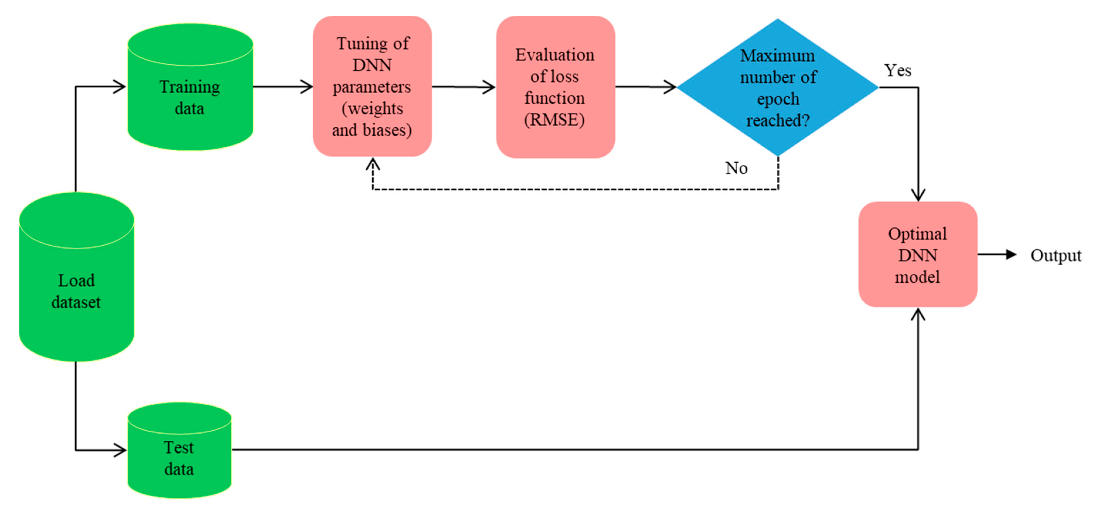
2.4. Deep Neural Network (DNN)

DNNs are artificial neural connections with multi-layered architecture [61]. The layers between input and output may automatically learn the non-linear patterns of data with several layers of abstraction. A DNN uses backpropagation (BP) learning algorithms to learn the complicated patterns in datasets. BP algorithms update the learning parameters of DNNs to compute the representation of each layer from the representations of preceding layer. It back propagates the output errors for fine-tuning of the network weights. The DNNs comprise an input layer, number of hidden layers and output layer. The DNNs are sensitive to its architecture and the value of hyperparameters such as wider vs. deeper networks, neuron count in hidden layers, activation function selection at each layer, optimizer, batch size, loss function, and epochs. DNNs are prone to underfitting and overfitting. The underfitting problem may be resolved by increasing the capacity of the network. However, regularization methods such as weight decay and early stopping with dropout and a weight constraint may cope with overfitting problems. Figure 1 shows the two-layered architecture of DNN for runoff prediction.

2.5. Extreme Learning Machine (ELM)

ELM is a type of least square based SLFNs which was proved for significant performance in classification and regression task [62,63]. Huang et al. [63] designed ELM by replacing a large number of neurons in the hidden layer with a kernel function. This technique provides good generalization performance with faster learning capability than some of the traditional machine learning algorithms [62]. Before training of the network, the output weights of the ELM are calculated based on the arbitrarily generated input weights and biases with defined number of the hidden layer neurons and activation function.

Figure 2 shows a single hidden layer neural network with ‘n’ number of input layer neurons, ‘l’ number of hidden layer neurons, ‘m’ number of output layer neurons. For example, if training dataset is {X_i, Y_i} then the input dataset is X_i = [X_i1, X_i2, …, X_in]^T ∈ ℝⁿ, the output dataset is Y_i = [Y_i1, Y_i2, …, Y_im]^T ∈ ℝ^m and i = 1, 2, …, l. The network of ELM can be mathematically modelled as:

$$t_j={\displaystyle \sum _{k=1}^l{\beta }_{k}g\left(w_k,b_k,z_j\right)}$$

(15)

where w_k is the input weights and b_k is the bias factor of the k^th hidden node which are the network learning parameters, z_j = [z_1j, z_2j, …, z_nj]^T, β_k = [β_k1, β_k2, …, β_k1]^T is the output weight of the k^th hidden node to the output nodes, g(w_k, b_k, z_j) is the k^th hidden node output with respect to the input z_j, t_j is the predicted output of the corresponding input z_j, j is the number of training samples which is denoted as q.

ELM produces w_k and b_k randomly and analytically estimates β by the Equation (16).

$$\underset{\beta }{\min }=\Vert H\ast \beta -T\Vert$$

(16)

The output weights are calculated using a linear equation [64] as:

$$\beta =H†Y$$

(17)

where H is the output matrix of the hidden layer (Equation (17)), H$†$ is the Moore–Penrose generalized inverse of H and Y = [y₁, y₂, …, y_q]^T is the actual target values of the training dataset.

$$H={\left[\begin{array}{ccc}g\left(w_1,b_1, x_1\right)& ‥& g\left(w_l,b_l, x_1\right)\\ :& & :\\ g\left(w_1,b_1, x_q\right)& ‥& g\left(w_l,b_l, x_q\right)\end{array}\right]}_{q\times l}$$

(18)

This paper uses radial basis function kernel ELM (RBF-ELM) where the number of hidden units need not to define before and feature mapping of hidden layer (g(w_k, b_k, z_j)) is hidden to the user [64,65].

2.6. Support Vector Regression (SVR), Artificial Neural Network (ANN) and Gradient Boosting Machine (GBM)

SVR is a kernel-based non-linear regression method, derived from support vector classification (SVC) by Boser et al. in 1992 [66,67]. It uses the principle of structural risk minimization, in order to minimize the upper bound of the generalization error instead of minimizing the prediction error on the training set. Basically, it tries to find the best regression hyperplane with smallest structural risk in high dimensional feature space. The more details about SVR can be found in [67].

The idea of ANN is derived from the known functionality of the human brain where a very large number of biological neurons are interconnected through the links. The various characteristics of biological neural network which is simulated by the ANN are the ability to handle non-linearity, noise and fault tolerance, massive parallelism, learning, and generalization capability. The ANN consists of an input layer, an output layer, and one or more hidden layers. The neurons in these layers are connected through the links. The weights of these links are adjusted during the learning process. In this paper, a back propagation algorithm is used to tune the parameters of ANN. The ANN may be able to model highly non-linear systems where the relationship among the variables is complex. The single hidden layered neural network is sufficient for hydrological modelling [68].

GBM is a numerical-based optimization algorithm, derived from gradient boosting classification by Friedman (2001). The main objective behind GBM is to minimize the loss function by iteratively adding a new decision tree (weak learner) at each step [69]. The new decision tree that is fitted to the current residual is added to the previous model in order to update the residual. This process continues until it reaches the maximum number of iterations provided by the researcher. At each iterative step the contribution of the added decision tree is shrunk using a parameter known as learning rate. The value of learning rate, lies between 0 and 1. In order to improve the predictive accuracy of the GBM some randomization is added to the fitting process. Randomization may include using randomly selected subsample instead of full training dataset.

3. Methodology

3.1. Study Area and Dataset Used

The daily rainfall and runoff data (15 years (2000–2015)) from two different benchmark stations of two catchments in the UK were obtained from the UK national river flow archive website (https://nrfa.ceh.ac.uk/ (accessed on 5 August 2019)). These two stations are part of the UK benchmark network (UKBN2) which are most suitable for interpretation and identification of long-term hydrological variability and change. The UK benchmark stations have all the full flow regime called low, medium and high flows. These catchments are sensibly free from disturbances of human like river engineering, urbanization, and water abstractions. Therefore, these are near-natural catchments and have climate-driven alterations in river flows.

The catchment of the river Teifi at Glanteifi from a wetter, cloudy, and windy region south-west Wales where the values of potential evapotranspiration are low relative to rainfall [70]. The winter months are wetter than the warm summer months. The monthly rainfall pattern increases from August, to peak in November–December, to January, then the pattern begins falling from February. The outlet of the basin is 893.6 km² and the river gauge at 5.2 m AOD (mean above ordnance datum). The primary river flow data measuring authority is Natural Resources Wales. The catchment has minor flow abstractions due to upland reservoirs and negligible agricultural demands. Therefore, the flow regime is natural. The factor affecting runoff are (i) reservoirs, and (ii) public water supply. The major portions of the catchment land cover are grassland (79%), woodland (12%), horticulture (4.74%), mountain (1.80%) and urban extent (2.83%). Catchment is mainly impermeable Ordovician and Silurian deposits. Over the land, dairy farming predominates in the south and hill farming in the upper catchment. Some forest with peaty soils on hills and is seasonally wet. The most of the lower areas have soils with permeable substrate.

The catchment of the river Fal at Tregony from dry, sunniest, mild winter, and cool summer region Cornwall country of south-west England where the values of potential evapotranspiration are higher relative to rainfall [70]. The monthly rainfall patterns increase from September to January [30]. The outlet of the basin is 87 km² and the river gauge at 6.9 m AOD. The primary river flow data measuring authority is the Environment Agency. Due to steep topography, the catchment has fast responses to the water events. The runoff coefficient is at a daily time step. The factor affecting runoff are (i) increased by effluent return, and (ii) reduced by industrial/agriculture use. The major portions of the catchment land cover are grassland (41.43%), horticulture (21.52%) with woodland (16.22%), mountain (0.18%) and urban extents (4.98%). The land use is low-grade agriculture and pasturage with some woodland. The catchment has no major changes. The statistics of catchments data is given in

Table 2. Statistics of dataset from two catchments.

Catchment		Mean	Sd.	Median	Min	Max	Skewness
Fal at Tragony	Discharge (m3/s)	2.03549	1.949909	1.37	0.208	48.24	3.69096
	Rainfall (mm/day)	3.37865	5.742897	0.6	0	55.9	2.693286
Teifi at Glanteifi	Discharge (m3/s)	29.6010	31.9316	18.290	0.7310	373.60	2.4780
	Rainfall (mm/day)	3.8631	6.2733	1	0	73.100	2.7719

.

The daily precipitation (mm per day) dataset was obtained from the center for ecology and hydrology-gridded estimates of areal rainfall (CEH-GEAR) [71,72]) which was interpolated to 1 km from the rain gauge data using the natural neighbor interpolation approach [71]. The uncertainty degree of the associated rainfall value depends on the mean distance to the nearest rain gauge station and the spatial variability of the rainfall. More details about the rainfall data can be found in [71]. Figure 3 shows daily discharge and rainfall data of the two basins.

A partial autocorrelation function (PACF) was used to select the number of preceding days runoff data for number of input features along with a previous day rainfall value. The proposed models predict the next day runoff value.

Furthermore, the highest correlated preceding runoff series and previous day rainfall series are pre-processed using discrete wavelet transform technique. The transformed time series data were used to predict the next day runoff value for both catchments. Further details of selected runoff and rainfall series with wavelet pre-processing are described in the model development section (Section 4).

3.2. Proposed EO-ELM and DNN

This study proposes a new empirical R-R model, called EO-ELM, where EO optimizes ELM learning parameters to find an optimal configuration of ELM for better prediction of runoff values. Here, the concentrations of EO are ELM learning parameters. The root mean square error (RMSE) is considered as objective function for EO. The best equilibrium candidate found by EO is considered as optimal configuration of ELM for prediction tasks.

In EO-ELM, initially all particles have no knowledge about the solution space. The collaboration of five equilibrium candidates help concentration updating process of particles. At initial periods of iteration, the equilibrium candidates are diverse in nature and exponential term (Equation (8)) produces large random numbers which helps particle to cover the entire solution space. Similarly, during end period of iterations, particles are surrounded equilibrium candidates which are in an optimal position with similar configuration. At these moments, the exponential term (Equation (8)) produces lower value of random number which helps fine tuning of candidate solutions. The algorithm of EO-ELM is shown in Algorithm 2.

Algorithm 2: The algorithm of EO-ELM

Input: 1. Training and testing dataset 2. Set hidden units and biases of ELM using initialization of EO populations 3. Assign of EO parameters value (a1 = 2, a2 = 1, GP = 0.5) (optimized parameters based on several trials of proposed model) Output: 4. Optimized hidden units and biases of ELM from best fitness of a EO equilibrium candidate 5. Get output weights of ELM using Moore Penrose Inverse 6. EO optimized ELM testing using test dataset Begin EO-ELM training 7. Initialize the fitness of four equilibrium candidates [fitness(${\overrightarrow{P}}_{eq\left[1\right]}$), fitness(${\overrightarrow{P}}_{eq\left[2\right]}$), fitness(${\overrightarrow{P}}_{eq\left[3\right]}$), fitness(${\overrightarrow{P}}_{eq\left[4\right]}$)] 8. for it = 1 to maximum iteration number do 9. for i = 1 to P do 10. Estimate the fitness of the ith particle 11.  if fitness(${\overrightarrow{P}}_i$) < fitness(${\overrightarrow{P}}_{eq\left[1\right]}$) 12.  Replace fitness(${\overrightarrow{P}}_{eq\left[1\right]}$) with fitness(${\overrightarrow{P}}_i$) and ${\overrightarrow{P}}_{eq\left[1\right]}$ with ${\overrightarrow{P}}_i$ 13.  elseif fitness(${\overrightarrow{P}}_i$) < fitness(${\overrightarrow{P}}_{eq\left[1\right]}$) & fitness(${\overrightarrow{P}}_i$) < fitness() 14.    Replace fitness(${\overrightarrow{P}}_{eq\left[2\right]}$) with fitness(${\overrightarrow{P}}_i$) and ${\overrightarrow{P}}_{eq\left[2\right]}$ with ${\overrightarrow{P}}_i$ 15.  elseif fitness(${\overrightarrow{P}}_i$) < fitness(${\overrightarrow{P}}_{eq\left[1\right]}$) & fitness(${\overrightarrow{P}}_i$) < fitness(${\overrightarrow{P}}_{eq\left[2\right]}$) & fitness(${\overrightarrow{P}}_i$) < fitness(${\overrightarrow{P}}_{eq\left[3\right]}$) 16.    Replace fitness(${\overrightarrow{P}}_{eq\left[3\right]}$) with fitness(${\overrightarrow{P}}_i$) and ${\overrightarrow{P}}_{eq\left[3\right]}$ with ${\overrightarrow{P}}_i$ 17.  elseif fitness(${\overrightarrow{P}}_i$) < fitness(${\overrightarrow{P}}_{eq\left[1\right]}$) & fitness(${\overrightarrow{P}}_i$) < fitness(${\overrightarrow{P}}_{eq\left[2\right]}$) & fitness(${\overrightarrow{P}}_i$) < fitness(${\overrightarrow{P}}_{eq\left[3\right]}$) & fitness(${\overrightarrow{P}}_i$) < fitness(${\overrightarrow{P}}_{eq\left[4\right]}$) 18.    Replace fitness(${\overrightarrow{P}}_{eq\left[4\right]}$) with fitness(${\overrightarrow{P}}_i$) and ${\overrightarrow{P}}_{eq\left[4\right]}$ with ${\overrightarrow{P}}_i$ 19.  end if 20.  end for 21.  ${\overrightarrow{P}}_{mean}$ = $\left({\overrightarrow{P}}_{eq\left[1\right]}+{\overrightarrow{P}}_{eq\left[2\right]}+{\overrightarrow{P}}_{eq\left[3\right]}+{\overrightarrow{P}}_{eq\left[4\right]}\right)/4$ 22. ${\overrightarrow{P}}_{eq, pool}=\left\{{\overrightarrow{P}}_{eq\left[1\right]}+{\overrightarrow{P}}_{eq\left[2\right]}+{\overrightarrow{P}}_{eq\left[3\right]}+{\overrightarrow{P}}_{eq\left[4\right]}+{\overrightarrow{P}}_{eq\left[mean\right]}\right\}$ (Equilibrium pool) 23. Allocate $t={\left(1-\frac{Iteration}{Max\_iteration}\right)}^{\left(a_2\times \frac{Iteration}{Max\_iteration}\right)}$      (Equation (6)) 24. for i = 1 to P do 25.  Random generation of vectors $\overrightarrow{\lambda }$ and $\overrightarrow{r}$         (Equation (8)) 26.  Random selection of equilibrium candidate from equilibrium pool 27.  Evaluate $\overrightarrow{F}=a_1\times sign\left(\overrightarrow{r}-0.5\right)\left[e^{-\overrightarrow{\lambda }t}-1\right]$   (Equation (8)) 28.  Evaluate $\overrightarrow{GCP}=\{\begin{array}{c}0.5\ast r_1 r_2\ge GP\\ 0 r_2<GP\end{array}$     (Equation (11)) 29.  Evaluate ${\overrightarrow{G}}_0=\overrightarrow{GCP}\ast \left({\overrightarrow{P}}_{eq}-\overrightarrow{\lambda }\times \overrightarrow{P}\right)$    (Equation (10)) 30.  Evaluate $\overrightarrow{G}={\overrightarrow{G}}_0\times \overrightarrow{F}$             (Equation (9)) 31.  $\overrightarrow{P}={\overrightarrow{P}}_{eq}+\left(\overrightarrow{P}-{\overrightarrow{P}}_{eq}\right)·\overrightarrow{F}+\frac{\overrightarrow{G}}{\overrightarrow{\lambda }V}\ast \left(1-\overrightarrow{F}\right)$ (Concentration updation)   (Equation (12)) 32. end for 33. end for 34. Set ELM optimal input weights and hidden biases using ${\overrightarrow{P}}_{eq\left[1\right]}$ (Best equilibrium candidate) 35. ELM testing

The authors propose and develop a DNN model for R-R modeling. Two hidden layers is considered for prediction of runoff values based on hit and trial approach. The gradient descent optimizer, called “adam”, is used for learning parameter (input weights and hidden weights and biases) tuning in DNN. The “adam” optimizer calculates each learning parameter of DNN based on the square of gradients. It adapts the learning rate for each weight of DNN by estimating first and second moment of gradient. The activation function used in hidden units is “relu”. The process flowchart of DNN is shown in Figure 4.

4. Model Development and Performance Metrics

The consideration of rainfall and runoff lag for model input combination is an important task in order to achieve better prediction performance. The best performance of ML models has been shown for an input combination in Nourani et al. [18] and Roy et al. [30] was two days lag of discharge (Q_t−2, Q_t−1), current day discharge (Q_t), and current day precipitation (P_t) are used to forecast the next-day discharge (Q_t+1) on daily R-R modeling. In this paper, auto-correlogram (ACF) and partial autocorrelation function (PACF) are used for selection of the optimal number of lags from the discharge series [72]. The optimal lags of the discharge series and a current day precipitation (P_t) are used to predict one-day ahead discharge value in the initial model development phase. The lag values of precipitation are already reflected in the lag discharge series. Figure 5a,c show ACF plot with 95% confidence bound for discharge series of Fal at Tregony and Teifi at Glanteifi, respectively, where both indicates (Figure 5a,c) that the correlation effect is weakened in subsequent lag values. In order to find a direct relationship (serial correlation) between number of lags with corresponding observation, PACF plots (Figure 5b,d) for Fal at Tregony and Teifi at Glanteifi, respectively) with 95% confidence are used in this study. PACF plots (Figure 5b,d) showed less correlation beyond some specific lag values or some specific lag values are highly correlated with corresponding observation. In this paper, the authors consider positive correlated lag values from PACF plots (Figure 5b,d). For the catchment Fal at Tregony (Figure 5b) 1, 2, 3, 4, 5, and 6 (6 preceding days) lags are considered for model input from the discharge series with current day precipitation value (here, 1-day lag). For the catchment of Teifi at Glanteifi (Figure 5d) 1, 3, 4, 5, and 6 (5 preceding days) lags are considered for model input from the discharge series with current day precipitation value (here, 1-day lag).

The original rainfall and runoff data is decomposed by a DWT method. The decomposed rainfall and runoff data are given to model input and next day discharge data are the corresponding output. Therefore, next day value of discharge is predicted from antecedent information of rainfall and runoff (2ⁿ-day mode and a maximum level of approximation mode, where n = 0,1, …,9). The decomposition runoff series (one preceding lag) is selected from PACF plots where the previous day lag of runoff shows (Figure 5b,d) the highest positive correlation (greater than 0.8) with next day runoff value for both the catchments. Due to previous lags of precipitations already being reflected in runoff series, the previous one day behind precipitation is selected as decomposition precipitation series. In this paper, the most commonly used smooth mother wavelet, called Daubechies (Db), in the hydrometeorological study is selected for model deployment. The number of levels for decomposition is determined by Equation (19), which is based on the mother wavelet and sample data points [73].

$$D_L={\log }_2[N/(2K-1)]$$

(19)

where $D_L$ is the maximum decomposition level, N is the number of sample data points, and K indicates the number of vanishing moments of a Db wavelet. A broader support of wavelet with higher vanishing moments are more appropriate for irregular and non-linear hydrological time series [74]. Therefore, an irregular wavelet Db7 is applied in this study where 7 is the vanishing moment. $D_L$ is estimated from two same data series for Fal at Tregony and Teifi at Glanteifi (N = 5838). Where K = 7, then for both time series data the estimated value of $D_L$ is found to be 9. It was showed that for $K\ge 7$, all approximations are similar [73].

The whole dataset of two catchments is divided into two parts: (i) training dataset (80%), and (ii) testing dataset (20%). The training dataset is used in the model calibration period and the calibrated model is used to predict the test dataset. In the training phase, the configuration of the ELM has been undertaken by initializing the input weights (w_l) and hidden neurons biases (b_i) using the population size of EO. After optimizing the decision variables by EO, output weights (β_l) are calculated analytically by the basic ELM procedure. Since the number of hidden neurons (l) influence the ELM performance, a trail was tested between the number of l versus mean square error (RMSE) (Equation (26)) to fix l. The training data set of 20 hidden neurons showed the better model performance for lags selection using PACF plots (Figure 5b,d). The final architecture of ELM with optimal number of discharge lags and P_t was set to n number of input neurons (n = 7, 6 for Fal at Tregony and Teifi at Glanteifi, respectively), 20 hidden neurons, and the number of training targets as output neurons. The main purpose of the use of EO and PSO is to optimize the input weight matrix (7 or 6 × 20) and hidden biases (20 × l) repeated within the number of training samples that minimize the error between predicted discharge and observed discharge value. That error value is calculated by Equation (20).

$$error=\frac{1}{q}{\displaystyle \sum _{j=1}^q{\left(Y^j-T^j\right)}^2}$$

(20)

where Y^j and T^j are the observed and predicted target value of the j^th sample, q is the total number of training sample. The total number of concentrations or features for EO and PSO particles is 160 (7 × 20 + 20) (for Fal at Tregony) and 140 (6 × 20 + 20) (for Teifi at Glanteifi) which are tuned during EO-ELM and PSO-ELM development for each run of EO and PSO, respectively. The size of the population is considered as 20 with 100 iterations for the best model performance for both catchments data with optimal discharge lags and current day precipitation. The optimal value of EO parameters are set a₁ = 2, a₂ = 1 and GP = 0.5. The optimal PSO parameters are set to C₁ = 1 and C₂ = 2. In the case of ELM, 20 hidden neurons are selected based on trials for both catchments. For KELM, 10 number of kernel parameter and C = 1 regularization coefficient is used based on trails for both datasets. The two-layered DNN model is considered for runoff prediction. After several trial and error, the number of hidden neurons in each layer are selected for best performance of DNN. Therefore, first and second hidden layers consist 10 and 5 neurons respectively for both catchments. The optimal batch size is 10 and epochs are set to 100 for DNN.

For wavelet-based sub-series decomposition of rainfall and discharge, nine sub-series and one approximation components feed into to the proposed model. The high-pass filters and low-pass filter rainfall and runoff are shown in Figure 6a–d for both catchments. For both catchments, total number of features or concentrations for EO and PSO particle are 525 (20 × 25 + 25) and 252 (20 × 12 + 12) which are tuned during WEO-ELM and WPSO-ELM development for Fal at Tregony and Teifi at Glanteifi respectively. The size of the population is considered as 20 with 100 iterations for the best model performance for both catchments data. The optimal value of EO parameters are set a₁ = 2, a₂ = 1 and GP = 0.5. The optimal PSO parameters are set to C₁ = 1 and C₂ = 2. After several trials of WELM, 250 hidden neurons are selected for Fal at Tregony and 50 hidden neurons are selected for Teifi at Glanteifi. For WKELM, 200 kernel parameters and C = 1 regularization coefficient is used based on trails for Fal at Tregony and 20,000 kernel parameters for Teifi at Glanteifi. The number of hidden neurons in two-layered WDNN are selected based on trials and error for best model performance. Therefore, first and second hidden layers consist 20 and 10 neurons respectively for both catchments. The optimal batch size is 10 and epochs are set to 100 for WDNN.

To evaluate the model’s performances, five statistical indicators have been used, namely (a) mean absolute error (MAE), (b) mean absolute percentage error (MAPE), (c) Nash–Sutcliffe efficiency (NSE), (d) coefficient of determination (R²), (e) RMSE and (f) variance account factor (VAF) which are formulated in Equations (21)–(26). The ‘hydroGOF’ R package [75] is used to compute the fitness values.

$$(\mathrm{a})MAE=\frac{1}{q}{\displaystyle {\sum }_{i=1}^q\left|Y_{O_i}-Y_{E_i}\right|}$$

(21)

$$(\mathrm{b})MAPE=\frac{1}{q}{\sum }_{i=1}^q\left|\frac{Y_{E_i}-Y_{O_i}}{Y_{E_i}}\right|\times 100$$

(22)

$$(\mathrm{c})NSE=\left(1-\frac{{\displaystyle \sum _{i=1}^q{\left(Y_{O_i}-Y_E{}_{{}_i}\right)}^2}}{{\displaystyle \sum _{i=1}^q{\left(Y_{O_i}-Y_{{\overline{O}}_i}\right)}^2}}\right)$$

(23)

$$(\mathrm{d})R^2={\left(\frac{{\displaystyle {\sum }_{i=1}^q\left(Y_{E_i}-Y_{{\overline{E}}_i}\right)\left(Y_{O_i}-Y_{{\overline{O}}_i}\right)}}{\sqrt{{\displaystyle {\sum }_{i=1}^q{\left(Y_{E_i}-Y_{{\overline{E}}_i}\right)}^2{\displaystyle {\sum }_{i=1}^n{\left(Y_{O_i}-Y_{\overline{O}}{}_{{}_i}\right)}^2}}}}\right)}^2$$

(24)

$$(\mathrm{e})RMSE=\sqrt{\frac{{\displaystyle \sum _{i=1}^q{\left(Y_{E_i}-Y_{O_i}\right)}^2}}{q}}$$

(25)

$$(\mathrm{f})VAF (\%)=\left(1-\frac{\mathrm{var}(Y_{E_i}-Y_{O_i})}{\mathrm{var}(Y_{E_i})}\right)\times 100$$

(26)

where $Y_{E_i}$ symbolized as the i^th estimated daily discharge using a model; $Y_{O_i}$ is the i^th observed daily discharge; $Y_{{\overline{E}}_i}$ is the average of the predicted daily discharge; $Y_{{\overline{O}}_i}$ is the average of the observed daily discharge and q is the total number of observations.

Furthermore, to ensure the trustworthiness and efficacy of eight models (ELM, KELM, PSO-ELM, EO-ELM, DNN, SVR, ANN and GBM), a quantitative assessment [76,77] is carried out.

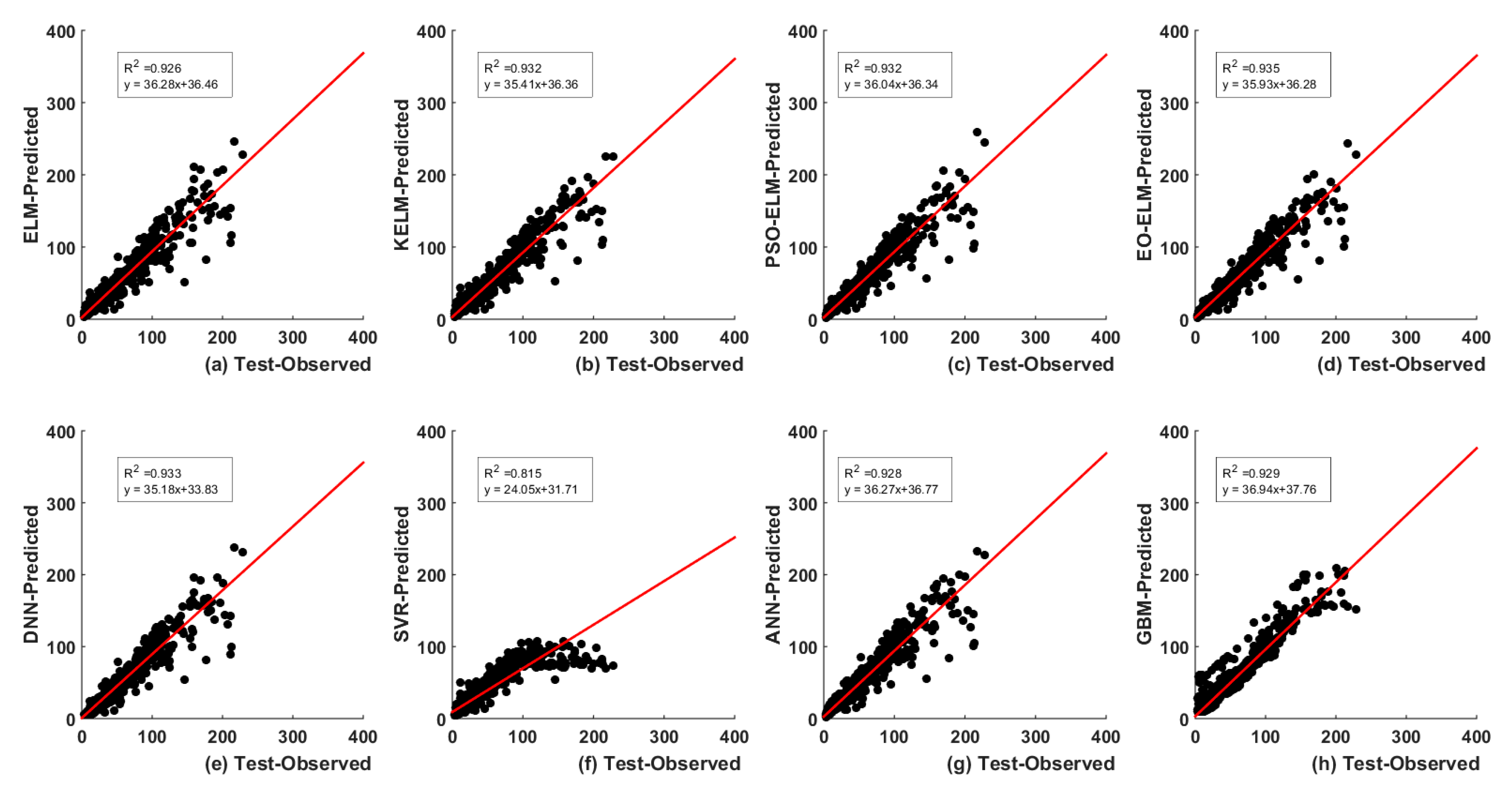
5. Results and Analysis

The proposed EO-ELM and DNN model applied to R-R modelling and six other well-known models, namely ELM, KELM, PSO-ELM, SVR, ANN and GBM, are considered for their comparison. To evaluate the performance of models, six evaluation indicators MAE, MAPE, NSE, R², RMSE and VAF have been used. Further, the ranking of models is assigned based on the value of each performance evaluation matric i.e., better the value, higher the ranking. In case of same value of matric, corresponding model ranking is decided based on the value priority of R² > RMSE > NSE > MAE.

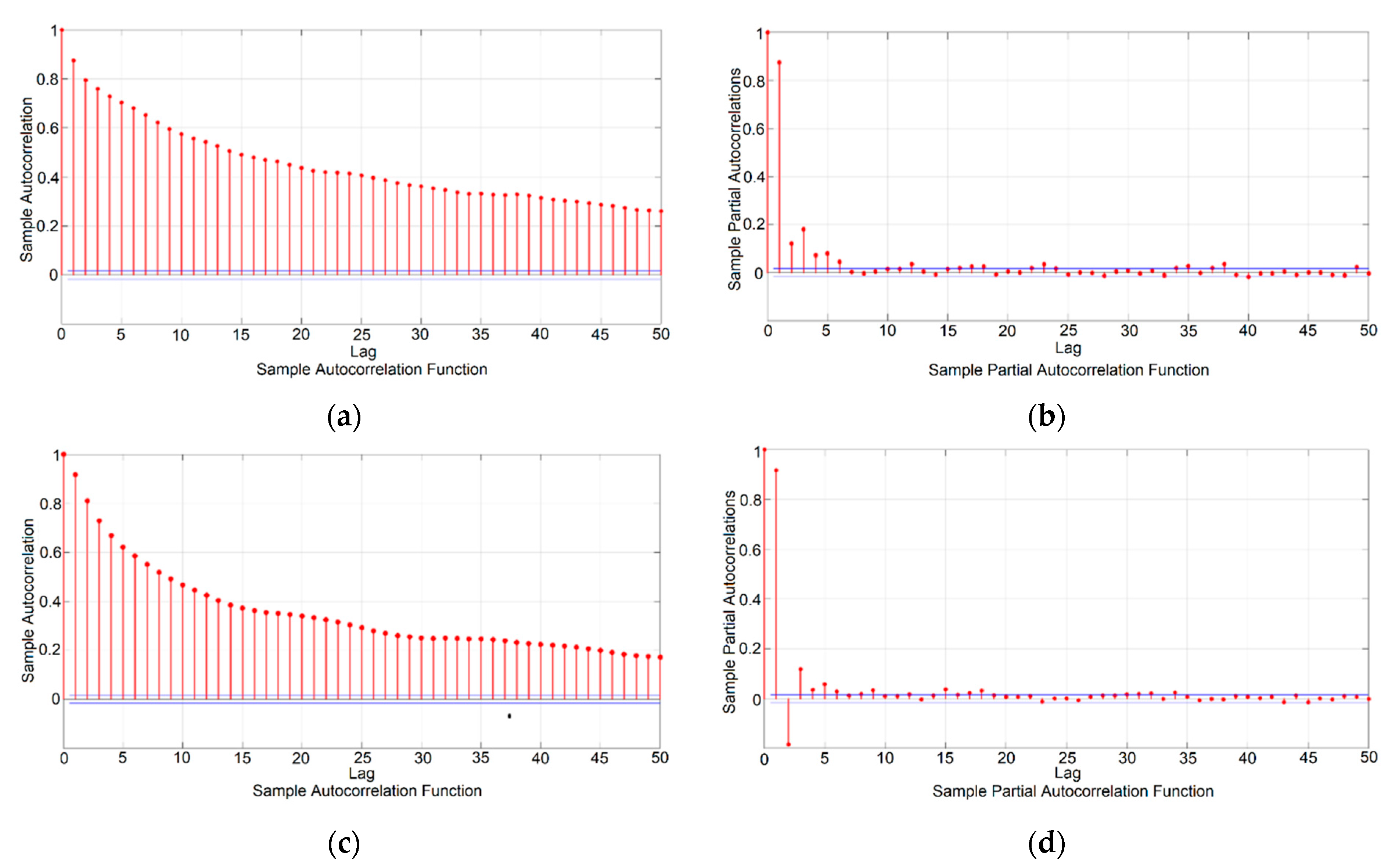
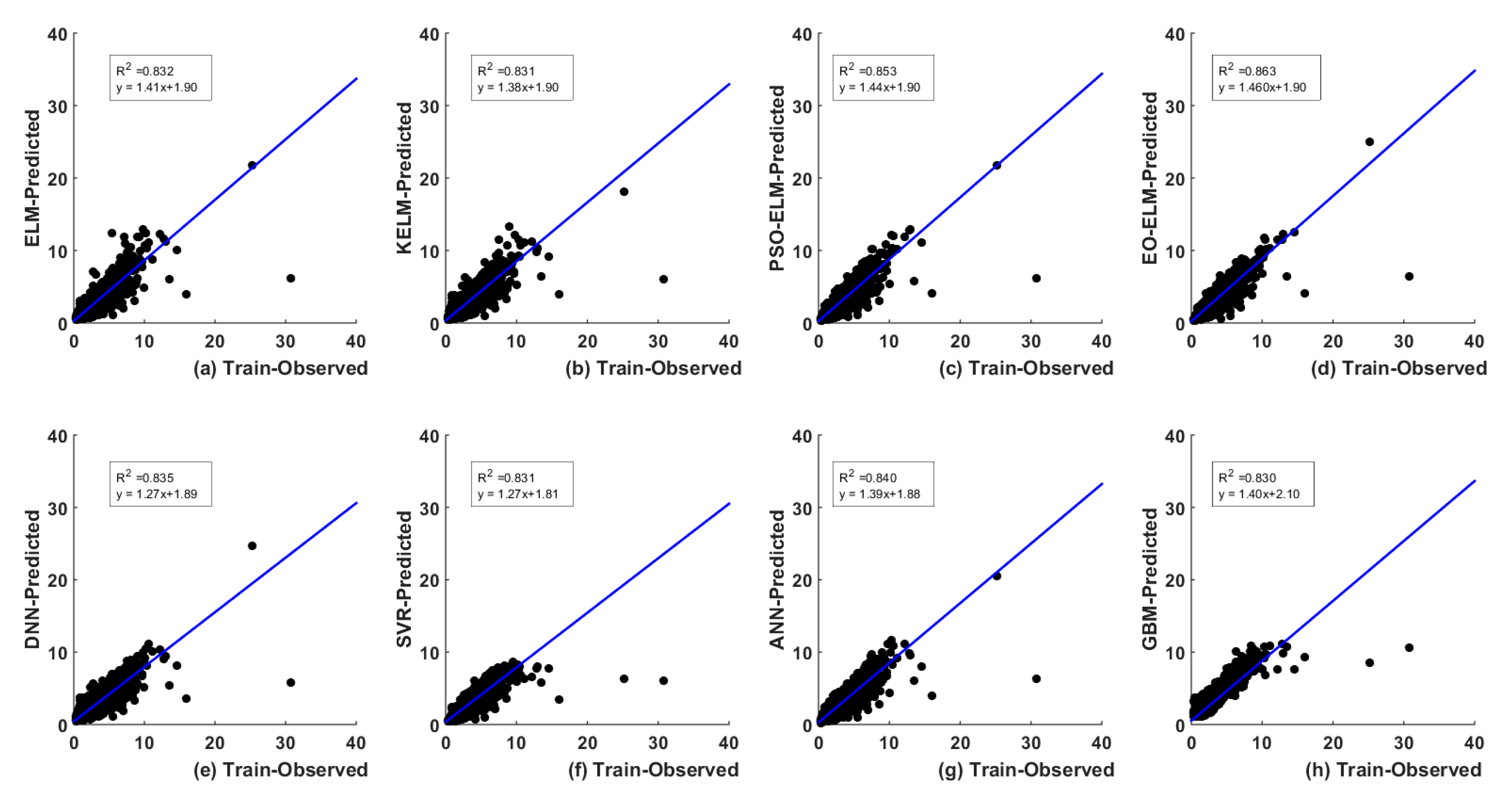
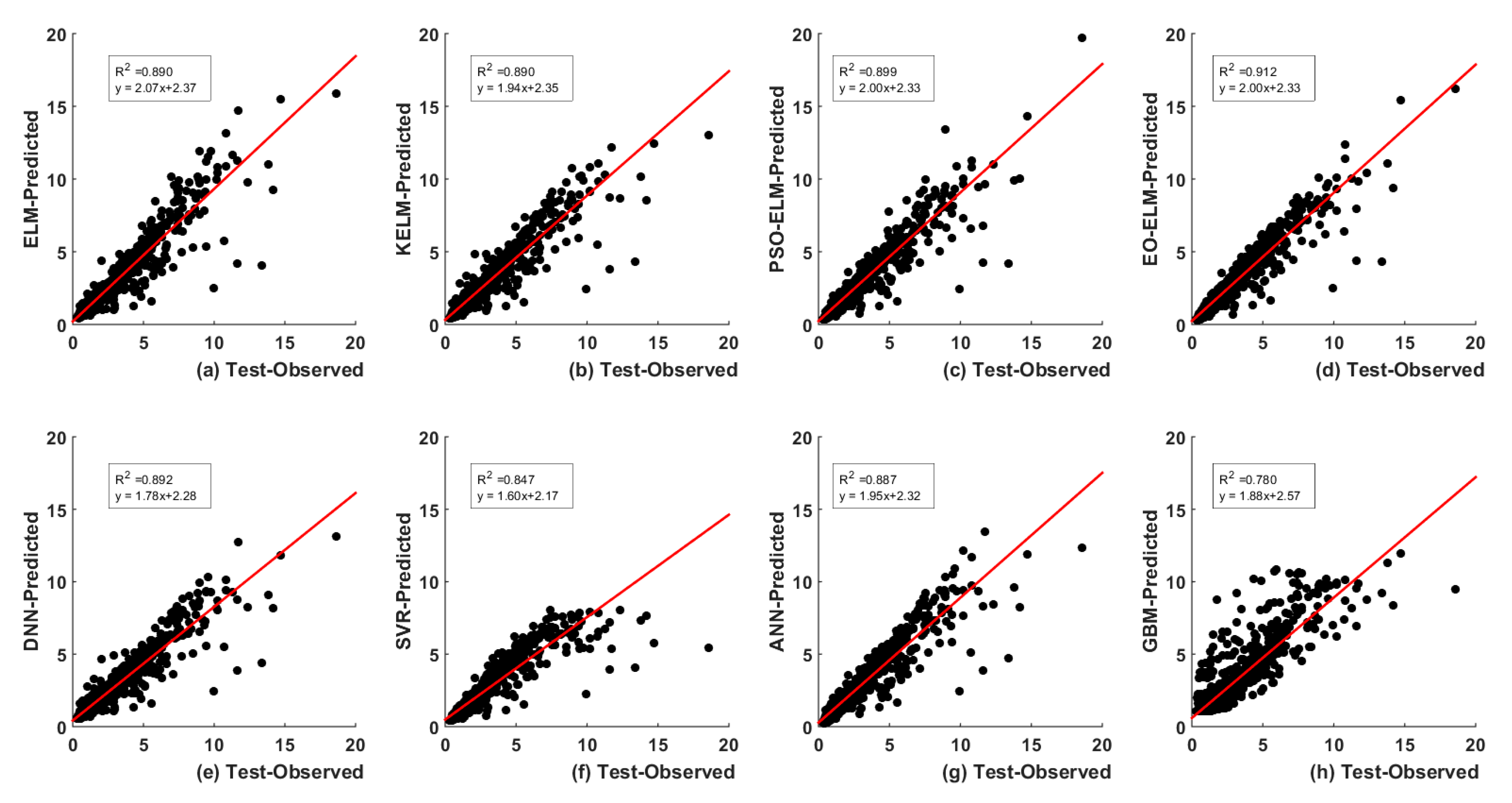
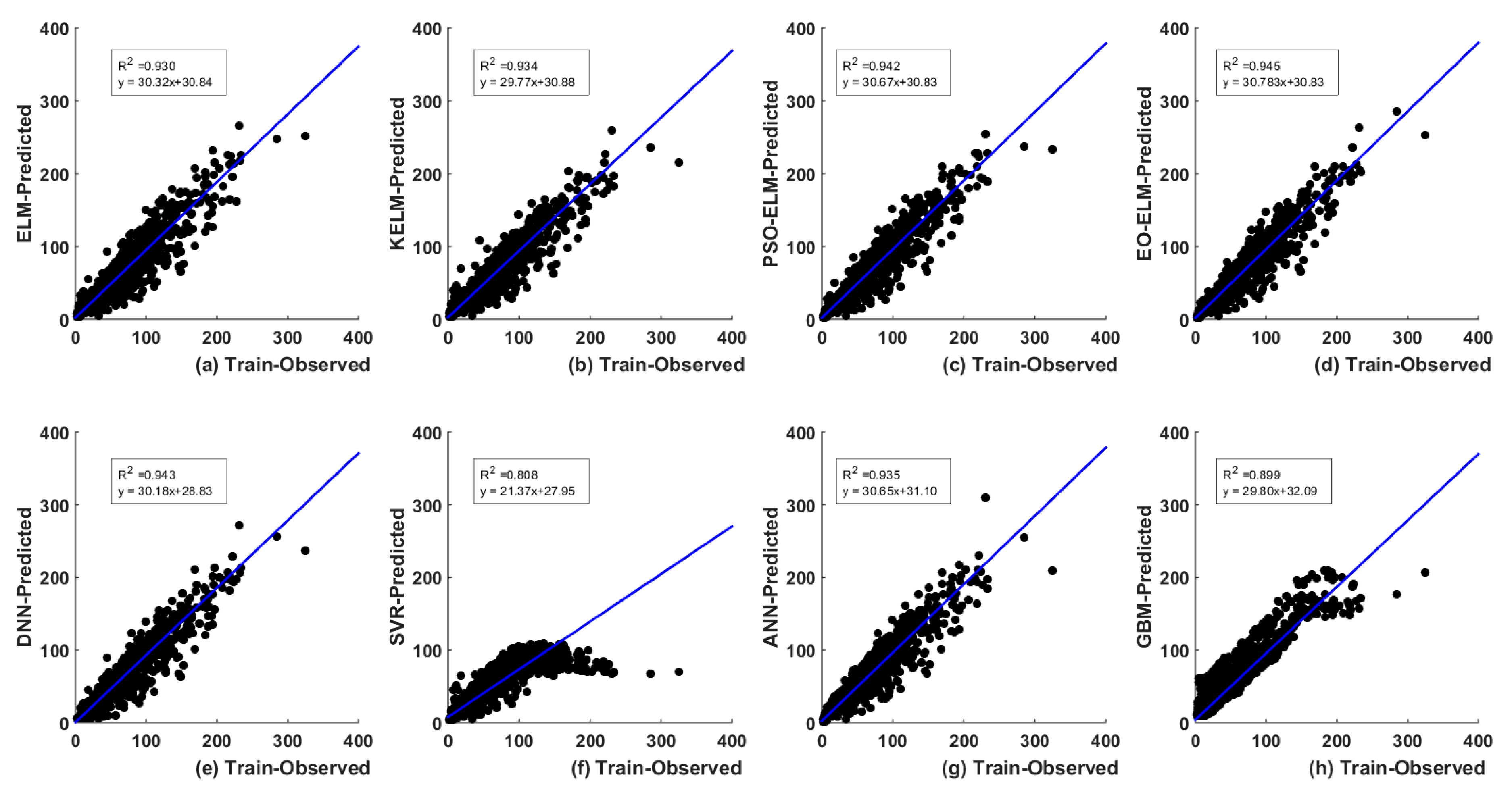
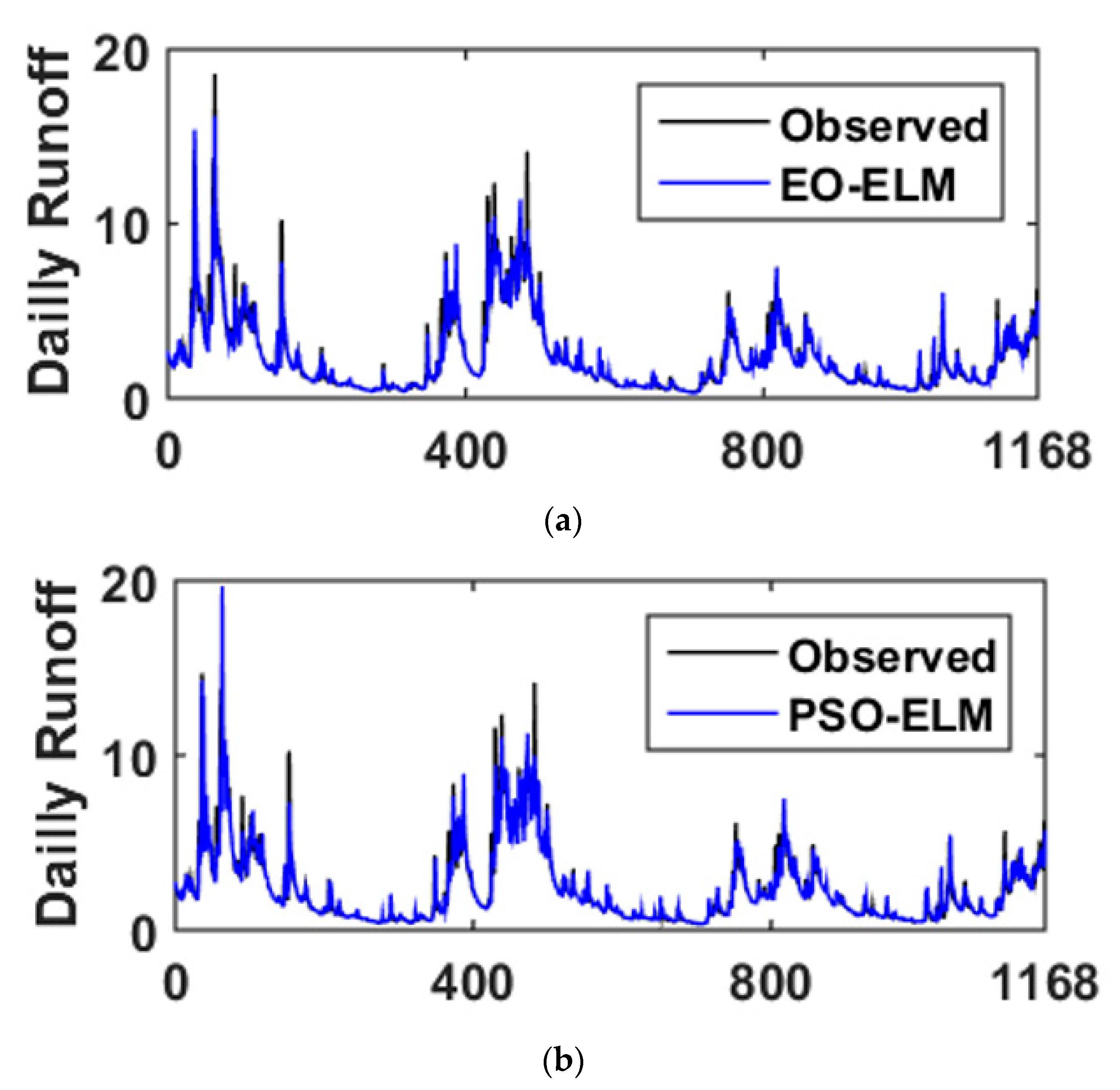
5.1. Optimal Lags-Based

Initially the optimal number of runoff lags from PACF plots and current day precipitation is used for model prediction of next day runoff value.

The performance of the models for the smaller catchment Fal at Tregony is shown in

Table 3. Lag-based models’ performance evaluation of the catchment Fal at Tregony.

		MAE	MAPE	NSE	R2	RMSE	VAF	TOTAL
ELM	Train	0.29	15.79	0.84	0.83	0.69	83.16
	Rank	5	3	5	4	5	5	27
	Test	0.35	15.58	0.95	0.89	0.75	88.93
	Rank	4	3	5	5	5	6	28
KELM	Train	0.29	15.30	0.84	0.83	0.70	83.06
	Rank	4	4	3	3	3	4	21
	Test	0.34	14.99	0.95	0.89	0.75	88.90
	Rank	6	4	6	6	6	5	33
PSO-ELM	Train	0.26	12.21	0.86	0.85	0.65	85.26
	Rank	7	7	7	7	7	7	42
	Test	0.31	11.29	0.95	0.90	0.72	89.85
	Rank	7	7	7	7	7	7	40
EO-ELM	Train	0.25	11.75	0.87	0.86	0.62	86.34
	Rank	8	8	8	8	8	8	48
	Test	0.29	11.18	0.96	0.91	0.68	91.13
	Rank	8	8	8	8	8	8	48
DNN	Train	0.32	20.53	0.84	0.84	0.70	82.71
	Rank	2	2	4	5	4	2	19
	Test	0.38	20.40	0.94	0.89	0.79	87.90
	Rank	2	2	3	3	3	3	16
SVR	Train	0.30	14.66	0.83	0.83	0.72	82.36
	Rank	3	5	2	2	2	1	15
	Test	0.35	12.95	0.91	0.85	0.97	82.39
	Rank	3	6	2	2	2	2	17
ANN	Train	0.28	13.71	0.85	0.84	0.68	83.93
	Rank	6	6	6	6	6	6	36
	Test	0.34	13.48	0.94	0.89	0.77	88.61
	Rank	5	5	4	4	4	4	26
GBM	Train	0.42	39.1	0.83	0.83	0.72	83.04
	Rank	1	1	1	1	1	3	8
	Test	0.66	47.97	0.89	0.78	1.09	77.72
	Rank	1	1	1	1	1	1	6

ELM: Extreme Learning Machine; KELM: Kernel ELM; PSO-ELM: Particle Swarm Optimization coupled ELM; EO-ELM: Equilibrium Optimizer coupled ELM; DNN: Deep Neural Network; SVR: Support Vector Regression; ANN: Artificial Neural Network; GBM: Gradient Boosting Machine.

. It is apparent that the proposed EO-ELM exhibits better prediction in the train and test phases compared to other applied models in terms of all measured matrices (Table 3). Furthermore, the prediction accuracy of DNN performed less compared to ELM, KELM, PSO-ELM, ANN, SVR and better compared to GBM (Table 3). It is evident from Table 3 that the EO-ELM model with rank 48 in both training and testing (having MAE = 0.25, MAPE = 11.75, NSE = 0.87, R2 = 0.86, RMSE = 0.62, VAF = 86.34 in training and MAE = 0.29, MAPE = 11.18, NSE = 0.96, R2 = 0.91, RMSE = 0.68, VAF = 91.13 in testing) achieved better results as compared to PSO-ELM model with rank 42 in training and 40 in testing (having MAE = 0.26, MAPE = 12.21, NSE = 0.86, R2 = 0.85, RMSE = 0.65, VAF = 85.26 in training and MAE = 0.31, MAPE = 11.29, NSE = 0.95, R2 = 0.90, RMSE = 0.72, VAF = 89.85 in testing). Figure 7 and Figure 8 exhibit better prediction performance of EO-ELM in the train (Figure 7d) and test (Figure 8d) cases respectively compared to other models with their linear equations for predicted and measured values.

Figure 9 shows the precise prediction line for EO-ELM (Figure 9a) against observed values in the test case compared to PSO-ELM (Figure 9b). The overfitting lines of peak discharge values are higher and underfitting lines of low discharge values for PSO-ELM are lower compared to EO-ELM (Figure 9). The Taylor plot (Figure 10a,b) confirms the better prediction performance of EO-ELM in terms of statistical comparison of all the models.

The performance of the models for the larger catchment of Teifi at Glanteifi is shown in

Table 4. Lag-based models’ performance evaluation of the catchment Teifi at Glanteifi.

		MAE	MAPE	NSE	R2	RMSE	VAF	TOTAL
ELM	Train	4.29	16.20	0.93	0.93	8.64	92.97
	Rank	3	5	3	3	3	3	20
	Test	5.15	15.02	0.95	0.93	10.81	92.60
	Rank	4	4	2	3	3	3	19
KELM	Train	4.06	16.32	0.93	0.93	8.37	93.39
	Rank	6	4	4	4	4	5	27
	Test	4.79	14.93	0.95	0.93	10.47	93.06
	Rank	6	5	6	6	6	6	35
PSO-ELM	Train	3.64	11.26	0.94	0.94	7.87	94.16
	Rank	7	8	7	7	7	6	42
	Test	4.59	12.44	0.95	0.93	10.45	93.10
	Rank	7	7	7	7	7	7	42
EO-ELM	Train	3.58	11.77	0.95	0.95	7.64	94.50
	Rank	8	7	8	8	8	8	47
	Test	4.46	11.67	0.95	0.94	10.18	93.46
	Rank	8	8	8	8	8	8	48
DNN	Train	4.17	17.99	0.94	0.94	8.04	94.28
	Rank	5	2	6	6	6	7	32
	Test	5.17	16.47	0.95	0.93	10.97	93.06
	Rank	3	2	2	2	2	5	16
SVR	Train	5.14	12.45	0.77	0.81	15.56	77.96
	Rank	2	6	1	1	1	1	12
	Test	7.56	13.78	0.82	0.82	20.11	76.18
	Rank	1	6	1	1	1	1	11
ANN	Train	4.29	16.8	0.93	0.94	8.31	93.49
	Rank	4	3	5	5	5	4	26
	Test	5.1	16.28	0.95	0.93	10.63	92.82
	Rank	5	3	4	4	4	2	22
GBM	Train	5.98	41.37	0.89	0.90	10.43	89.89
	Rank	1	1	2	2	2	2	10
	Test	6.13	34.71	0.95	0.93	10.55	92.93
	Rank	3	1	5	5	5	4	24

. It is apparent that the proposed EO-ELM exhibits better prediction in test phase compared to other applied models in terms of all measured matrices (Table 4). Furthermore, the prediction accuracy of DNN performed less compared ELM, KELM PSO-ELM, ANN and better compared to SVR, GBM (Table 4). It is evident from Table 4 that EO-ELM model with rank 48 in training and 47 in testing (having MAE = 3.58, MAPE = 11.77, NSE = 0.95, R2 = 0.95, RMSE = 7.64, VAF = 94.50 in training and MAE = 4.46, MAPE = 11.67, NSE = 0.95, R2 = 0.94, RMSE = 10.18, VAF = 93.46 in testing) achieved better results as compared to PSO-ELM model with rank 42 in both training and testing (having MAE = 0.64, MAPE = 11.26, NSE = 0.94, R2 = 0.94, RMSE = 7.87, VAF = 94.16 in training and MAE = 4.5, MAPE = 12.44, NSE = 0.95, R2 = 0.93, RMSE = 10.45, VAF = 93.10 in testing).

Figure 11 (refer supp) and Figure 12 (refer supp) exhibit better prediction performance of EO-ELM in train (Figure 11d) and test (Figure 12d) cases, respectively, compared to other models with their linear equations for predicted and measured values. The Taylor plot (Figure 13a,b) confirms the better prediction performance of EO-ELM in terms of statistical comparison of all models.

In the initial period (PACF-based selected lags) of model development, models give a distinct predictive performance for the two different catchment sizes, and characteristics result in hydrological responses to precipitation. The different values of statistical parameters of the datasets shown in (Table 2). However, the EO-ELM performed better in the large catchment Teifi at Glanteifi (R² = 0.935) which has a sensibly natural flow regime with minor flow abstractions due to the upland reservoirs and negligible agricultural demands compared to the catchment Fal at Tregony (R² = 0.91) which has moderate modification to flow due to steep topography, increasing runoff from effluent returns, and runoff reduces by industrial and agricultural abstractions that might be due to smaller watershed where the smaller catchment characteristics is more sensitive than larger watershed.

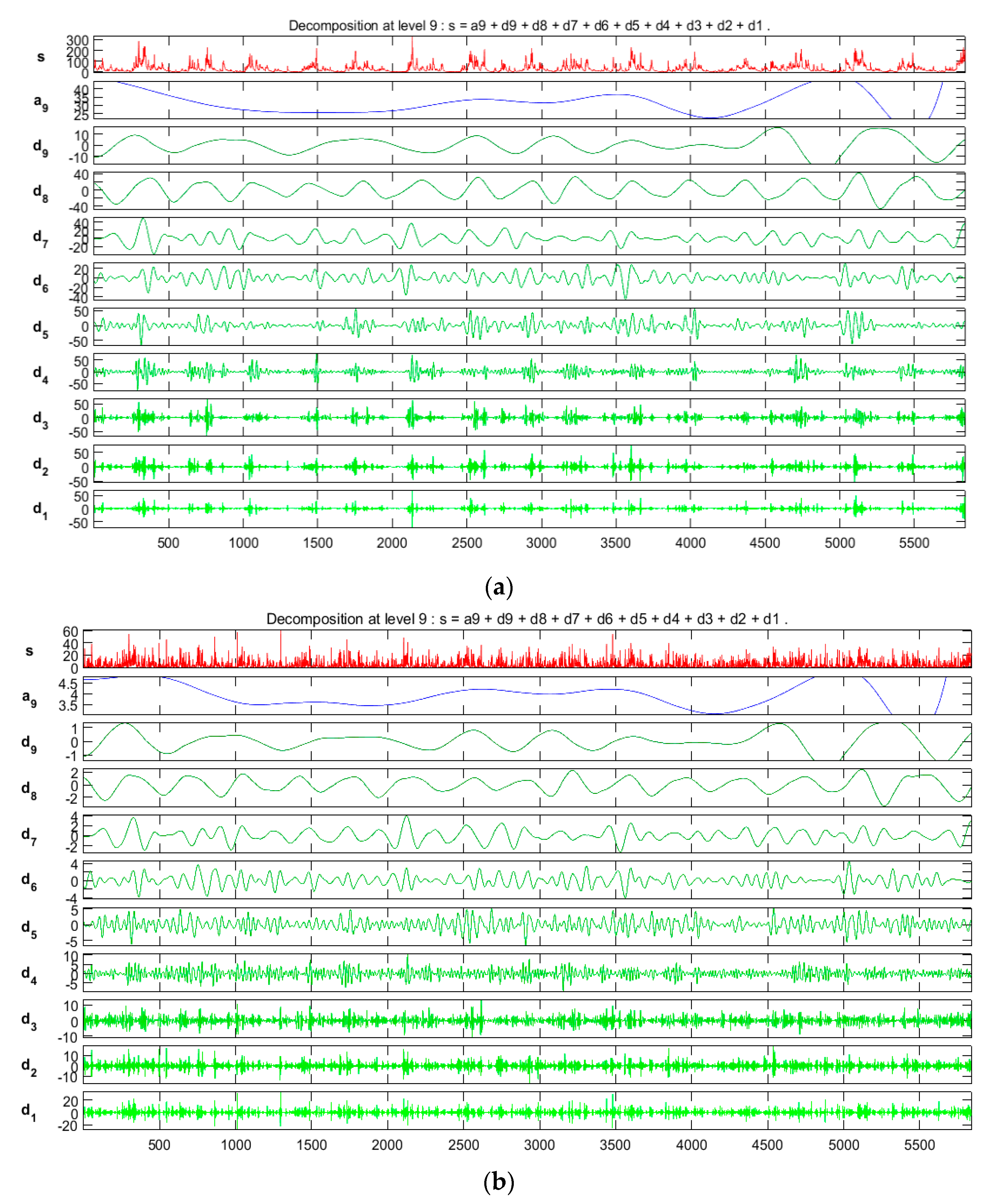
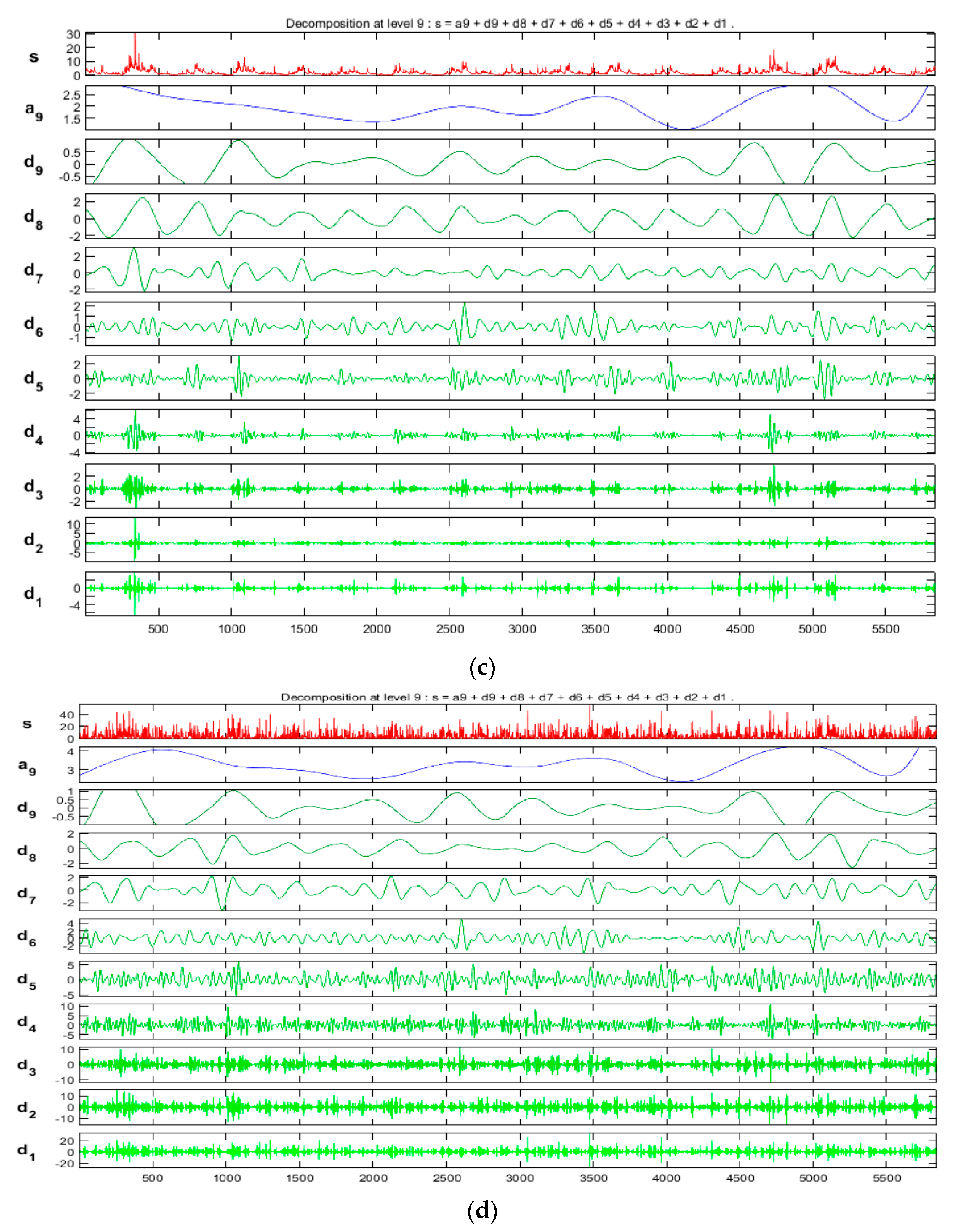
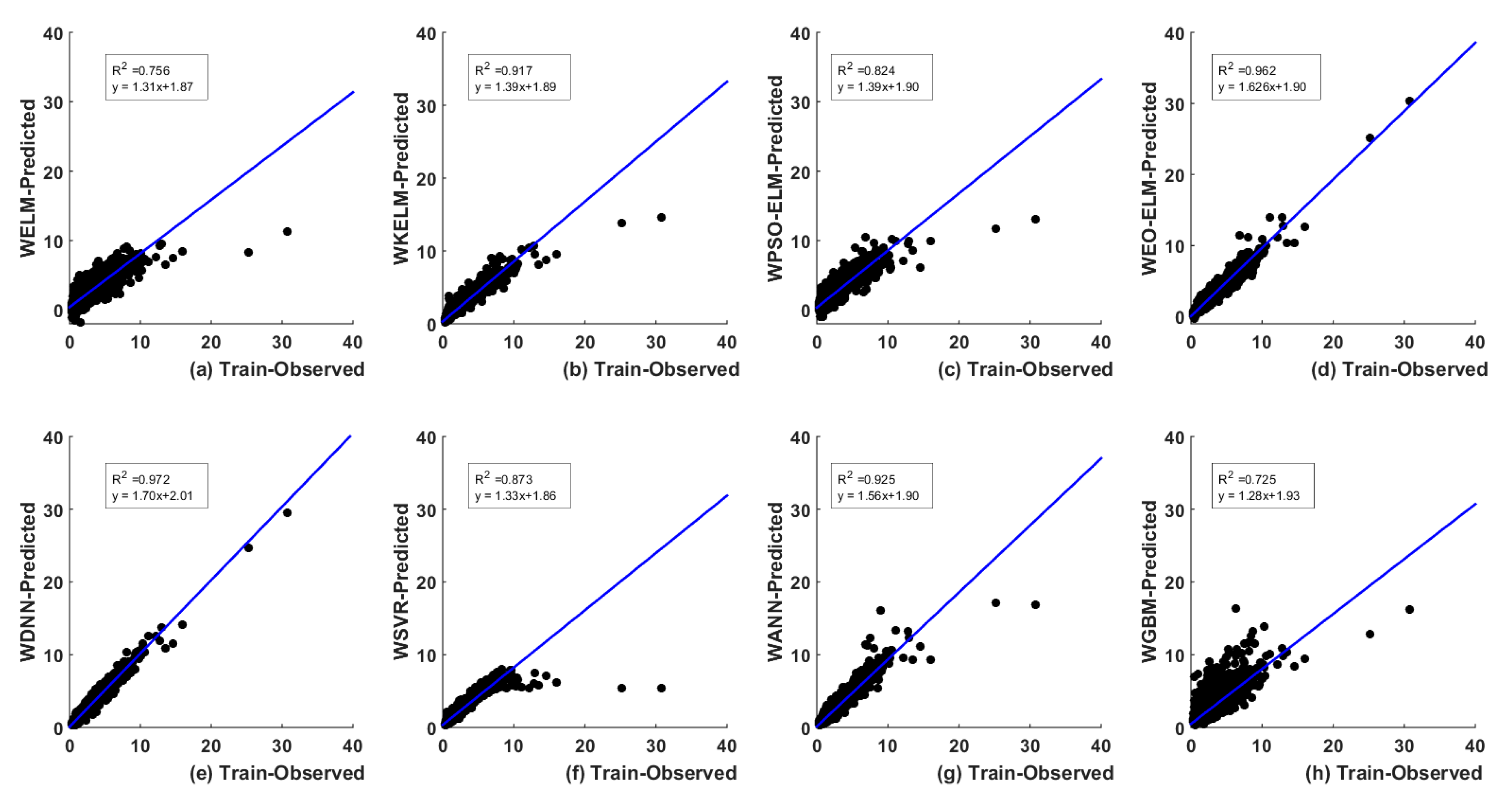
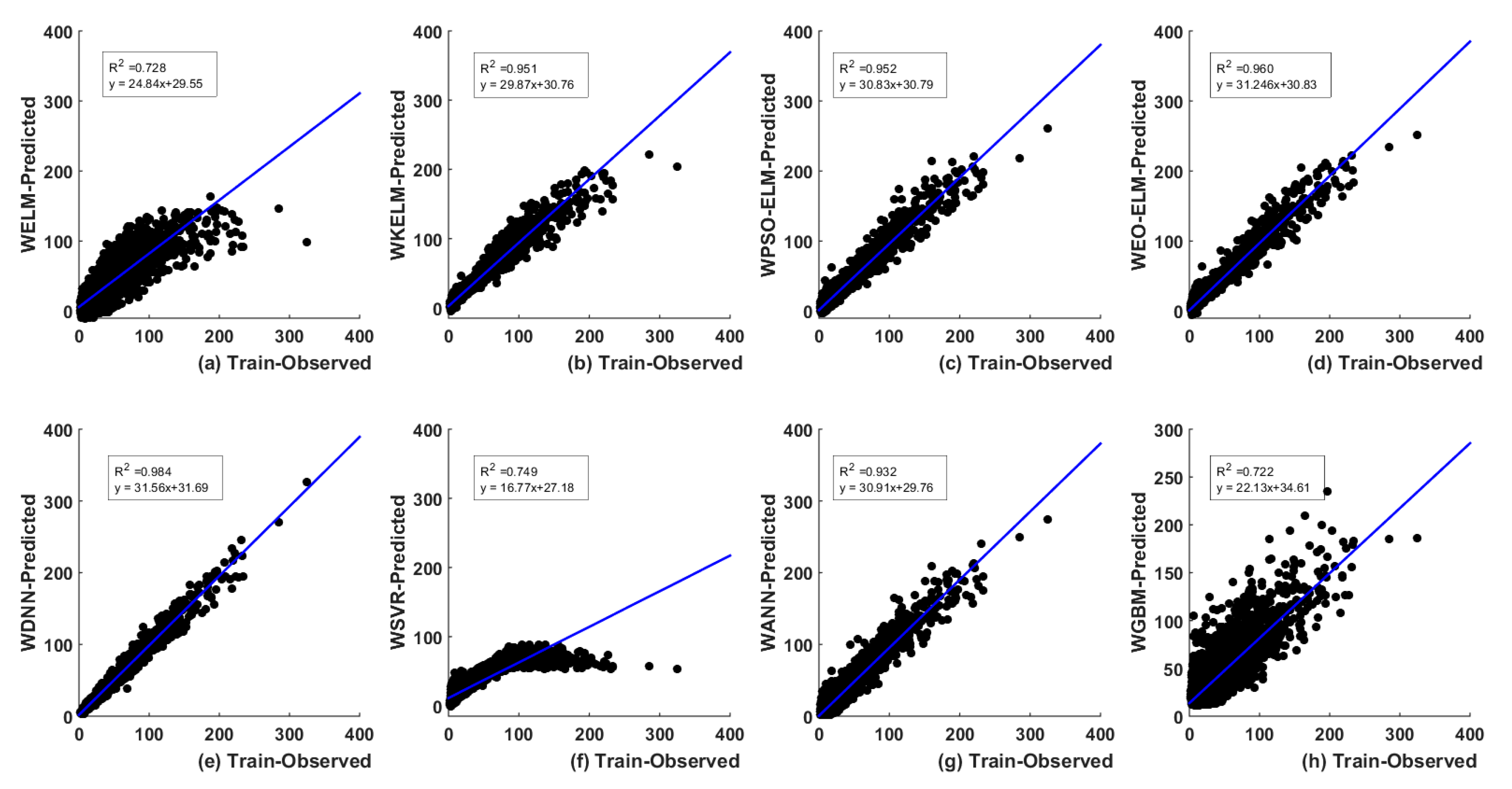
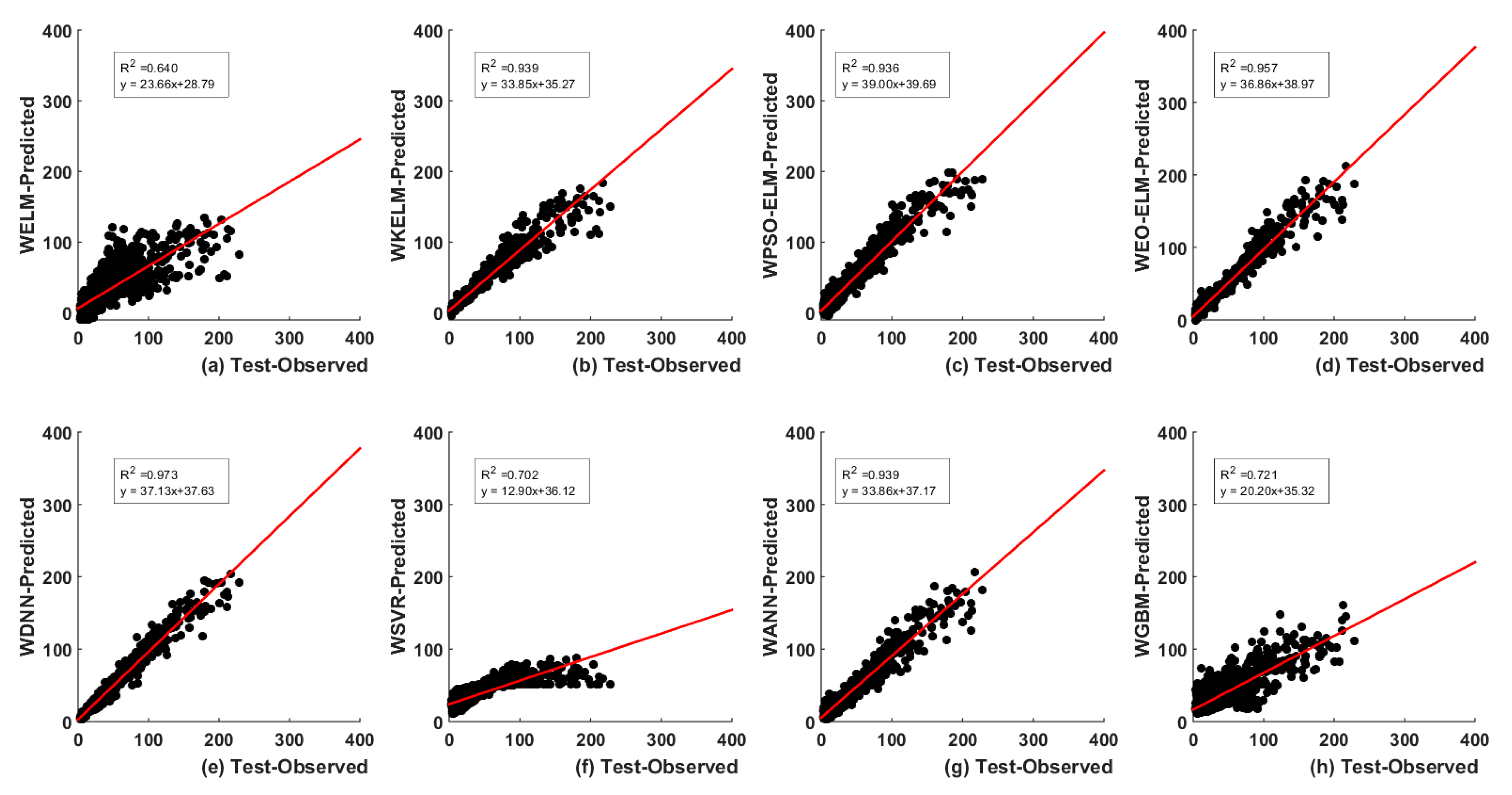
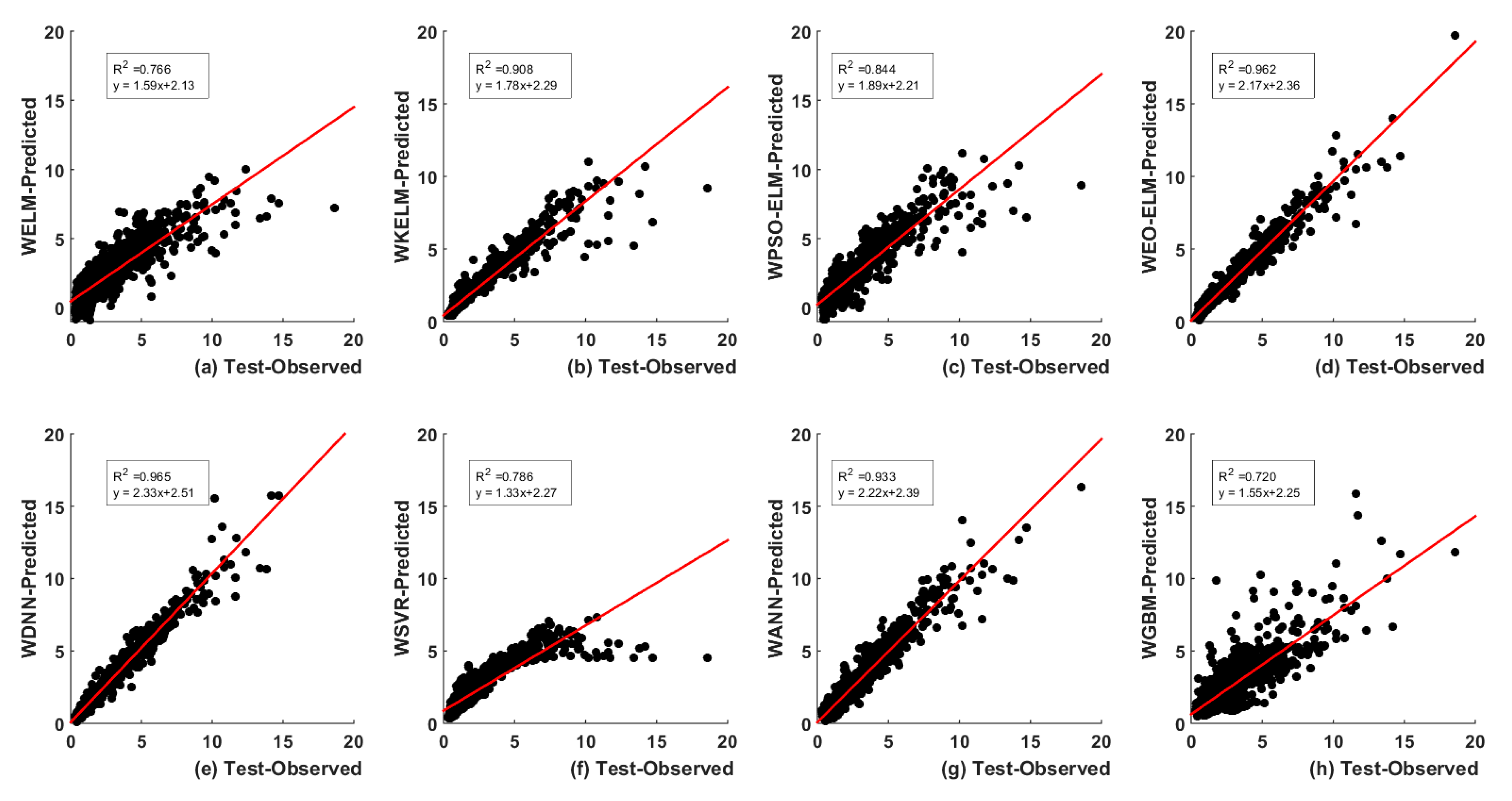
5.2. Discrete Wavelet Transform (DWT)-Based

In UK catchments, the discharge prediction using rainfall and runoff modelling is a challenging task [60,78,79]. In order to achieve better prediction result of runoff in both catchments, the authors used the DWT-based time series data pre-processing technique in the rainfall and runoff dataset. Both current day rainfall and current day runoff (the highest correlated runoff data which has greater than 0.8 correlation observed from PACF plots for both catchments (Figure 5b,d) series are decomposed by estimated optimal number of sub-series (D1 to D9) with an approximation (A9) using Equation (19). The decomposed series of rainfall and discharge data are fed into models and next day discharge value is the predicted output value.

The performance of the wavelet-based models for the catchment Fal at Tregony is shown in

Table 5. Wavelet-based models’ performance evaluation of the catchment Fal at Tregony.

		MAE	MAPE	NSE	R2	RMSE	VAF	TOTAL
WELM	Train	0.51	36.00	0.77	0.76	0.84	75.53
	Rank	3	3	2	2	2	2	14
	Test	0.72	41.36	0.88	0.77	1.13	76.05
	Rank	2	1	3	2	3	3	14
WKELM	Train	0.72	41.36	0.91	0.92	0.51	90.75
	Rank	1	1	5	5	5	5	22
	Test	0.30	12.78	0.95	0.91	0.75	89.18
	Rank	6	7	5	5	5	5	33
WPSO-ELM	Train	0.42	29.06	0.84	0.82	0.71	82.36
	Rank	4	4	3	3	3	3	20
	Test	0.53	31.37	0.92	0.84	0.91	84.40
	Rank	4	3	4	4	4	4	23
WEO-ELM	Train	0.18	11.26	0.96	0.96	0.33	96.19
	Rank	8	8	7	7	7	7	44
	Test	0.24	11.81	0.98	0.96	0.47	96.18
	Rank	8	8	7	7	7	8	45
WDNN	Train	0.21	13.60	0.97	0.97	0.31	97.09
	Rank	7	7	8	8	8	8	46
	Test	0.30	15.70	0.98	0.97	0.44	96.04
	Rank	7	6	8	8	8	7	43
WSVR	Train	0.40	27.03	0.87	0.87	0.62	86.47
	Rank	5	5	4	4	4	4	26
	Test	0.55	26.44	0.87	0.79	1.17	73.65
	Rank	3	4	2	3	1	2	15
WANN	Train	0.24	16.24	0.93	0.93	0.46	92.46
	Rank	6	6	6	6	6	6	36
	Test	0.40	22.86	0.96	0.93	0.60	93.11
	Rank	5	5	6	6	6	6	34
WGBM	Train	0.53	36.09	0.74	0.73	0.89	72.42
	Rank	3	2	1	1	1	1	9
	Test	0.78	40.50	0.86	0.72	1.20	71.78
	Rank	1	2	1	1	2	1	8

. It is apparent that the proposed WEO-ELM and WDNN exhibits better prediction in train and test phase compared to others in terms of all measured matrices (Table 5). For this catchment, the prediction accuracy of WDNN is comparable to WEO-ELM and better compared to WELM, WKELM, WPSO-ELM, WSVR, WANN and WGBM (Table 5). It is evident from Table 5 that WEO-ELM model with rank 44 in training and 45 in testing (having MAE = 0.18, MAPE = 11.26, NSE = 0.96, R² = 0.96, RMSE = 0.33, VAF = 96.19 in training and MAE = 0.24, MAPE = 11.81, NSE = 0.98, R² = 0.96, RMSE= 0.47, VAF = 96.18 in testing) which is comparable with WDNN model with rank 46 in training and 43 in testing (having MAE = 0.21, MAPE = 13.60, NSE = 0.97, R² = 0.97, RMSE = 0.31, VAF = 97.09 in training and MAE = 0.30, MAPE = 15.70, NSE = 0.98, R² = 0.97, RMSE = 0.44, VAF = 96.04 in testing). Figure 14 and Figure 15 exhibit better prediction performance of WEO-ELM and WDNN in the train and test case respectively compared to other models with their linear equations for predicted and measured values.

Figure 14d,e shows better prediction in train case for WEO-ELM and WDNN respectively against observed values. From Figure 14a–h, it is confirmed that WDNN (R² = 0.972) performed better compared to other six ML models. Similarly, Figure 15d,e shows better prediction in test case for WEO-ELM and WDNN, respectively, against observed values. From Figure 15a–h, it is confirmed that WDNN (R² = 0.965) performed better compared to the other six ML models. The Taylor plots (Figure 16a,b) confirm the better prediction performance of WDNN in terms of the statistical comparison of all models.

The performance of the wavelet-based models for the catchment Teifi at Glanteifi is shown in

Table 6. Wavelet-based models’ performance of the catchment Teifi at Glanteifi.

		MAE	MAPE	NSE	R2	RMSE	VAF	TOTAL
WELM	Train	11.18	60.20	0.73	0.73	17.07	72.68
	Rank	2	2	3	2	3	3	15
	Test	16.11	60.14	0.72	0.64	25.32	63.70
	Rank	2	3	2	1	2	2	12
WKELM	Train	3.76	16.53	0.95	0.95	7.32	94.95
	Rank	7	7	5	5	5	5	34
	Test	5.09	18.56	0.95	0.94	10.57	93.12
	Rank	7	7	4	4	4	4	30
WPSO-ELM	Train	4.53	26.26	0.95	0.95	7.15	95.19
	Rank	5	4	6	6	6	6	33
	Test	7.42	40.87	0.95	0.94	10.51	93.36
	Rank	4	5	5	5	5	6	30
WEO-ELM	Train	3.88	21.58	0.96	0.96	6.52	95.99
	Rank	6	6	7	7	7	7	40
	Test	5.12	25.49	0.97	0.96	8.44	95.67
	Rank	6	6	7	7	7	7	40
WDNN	Train	2.65	13.75	0.98	0.98	4.26	98.36
	Rank	8	8	8	8	8	8	48
	Test	3.96	17.21	0.98	0.97	6.65	97.20
	Rank	8	8	8	8	8	8	48
WSVR	Train	7.22	25.30	0.67	0.75	18.90	67.59
	Rank	3	5	1	3	1	1	14
	Test	17.69	99.68	0.65	0.70	28.05	49.98
	Rank	1	1	1	3	1	1	8
WANN	Train	6.21	38.07	0.93	0.93	8.60	93.13
	Rank	4	3	4	4	4	4	23
	Test	6.94	41.07	0.95	0.94	10.39	93.14
	Rank	5	4	6	6	6	5	32
WGBM	Train	12.84	99.42	0.71	0.72	17.66	71.94
	Rank	1	1	2	1	2	2	9
	Test	15.78	83.81	0.76	0.72	23.24	65.86
	Rank	3	2	3	3	3	3	17

. It is apparent that the proposed WDNN exhibits better prediction in train and test phase compared to others in terms of all measured matrices (Table 6). For this catchment, the prediction accuracy of WEO-ELM follows WDNN and better compared to WKELM, WPSO-ELM, WELM, WANN, WSVR, and WGBM (Table 6). It is evident from Table 6 that WDNN model with rank 48 in both training and testing (having MAE = 2.65, MAPE = 13.75, NSE = 0.98, R2 = 0.98, RMSE = 4.26, VAF = 98.36 in training and MAE = 3.96, MAPE = 17.21, NSE = 0.98, R2 = 0.97, RMSE = 6.65, VAF = 97.20 in testing) achieved better results as compared to WEO-ELM model with rank 40 in both training and testing (having MAE = 3.88, MAPE = 21.58, NSE = 0.96, R2 = 0.96, RMSE = 6.52, VAF = 95.99 in training and MAE = 5.12, MAPE = 25.49, NSE = 0.97, R2 = 0.96, RMSE = 8.44, VAF = 95.67 in testing). Figure 17 and Figure 18 exhibit better prediction performance WDNN in train and test case respectively compared to other models with their linear equations for predicted and measured values. Interestingly, the EO algorithm adequately optimized ELM parameters than the PSO algorithm and enhanced the performance of ELM sufficiently compared to PSO. The Taylor plot (Figure 19a,b) confirms the better prediction performance of WDNN followed by WEO-ELM in terms of statistical comparison of all models.

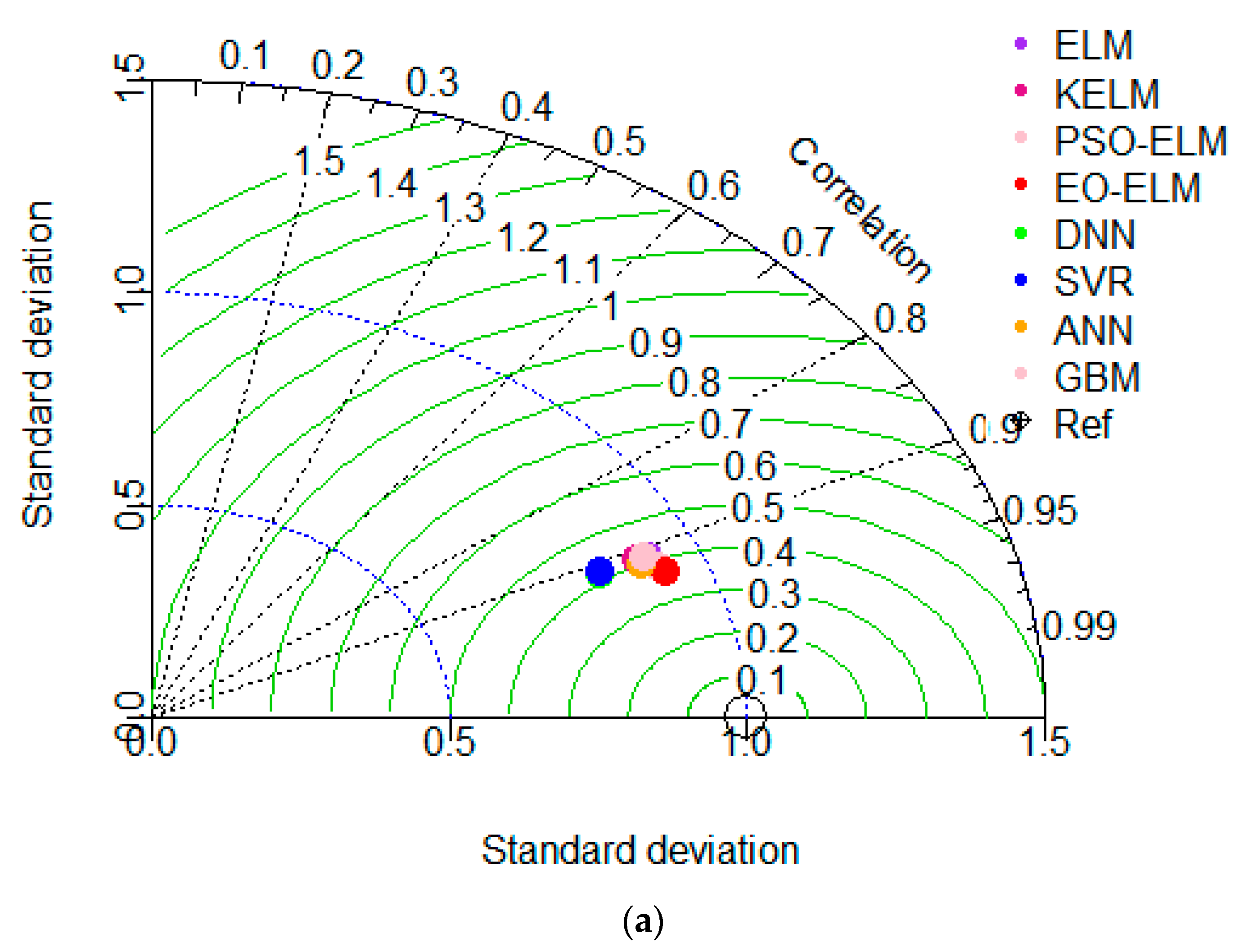
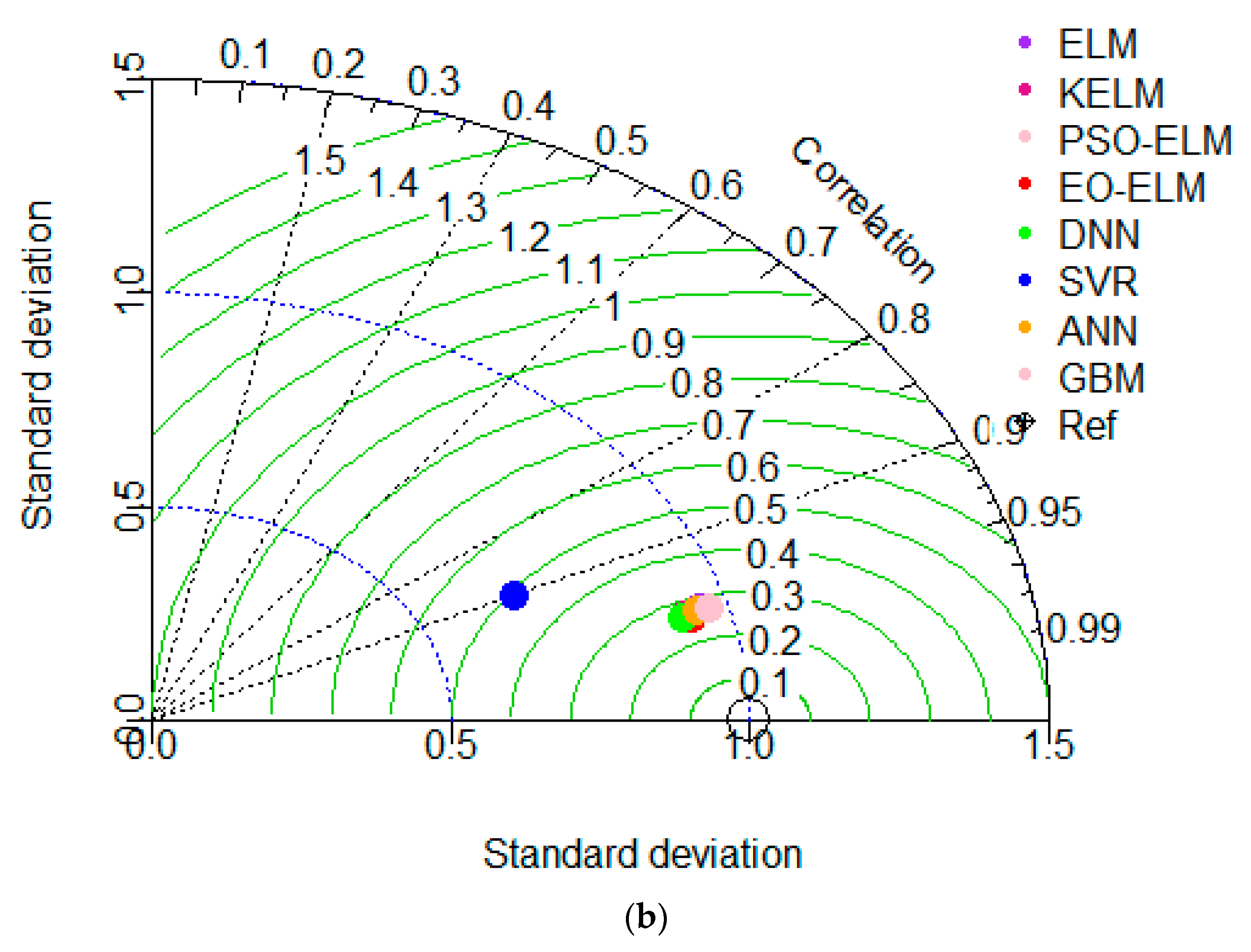
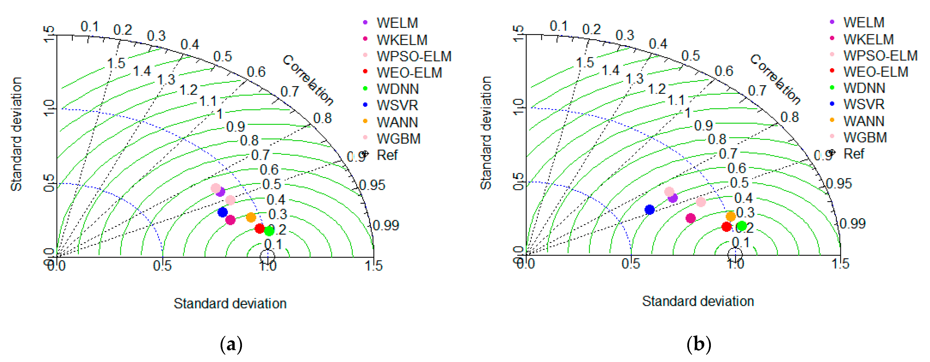
5.3. Uncertainty Analysis (UA) of Models

Both training and testing observed samples were considered for logical comparison of predicted discharge values for these models. The quantification of uncertainty and its analysis using appropriate variable is useful for knowing the technical contribution in a decision-making environment. In this study, the knowledge base for analysis was observed and predicted discharge values. Initially the error $(e_i)$ between the observed ($Y_{O_i}$) and predicted ($Y_{E_i}$) value is formulated using Equation (27).

$$e_i=\left|Y_{O_i}-Y_{E_i}\right|$$

(27)

Then mean ($e_{\mu })$, standard deviation (SD) $\left({\sigma }_e^2\right)$, standard error (SE), upper bound (UB), lower bound (LB) and width of confidence (WCB) bound of error are calculated. The margin of error (ME) is estimated with 95% confidence interval with 0.05 level of significance $\left(1-\alpha \right)$. The smaller value of mean, UB, LB, SE, ME and WCB indicates better accuracy of a prediction model.

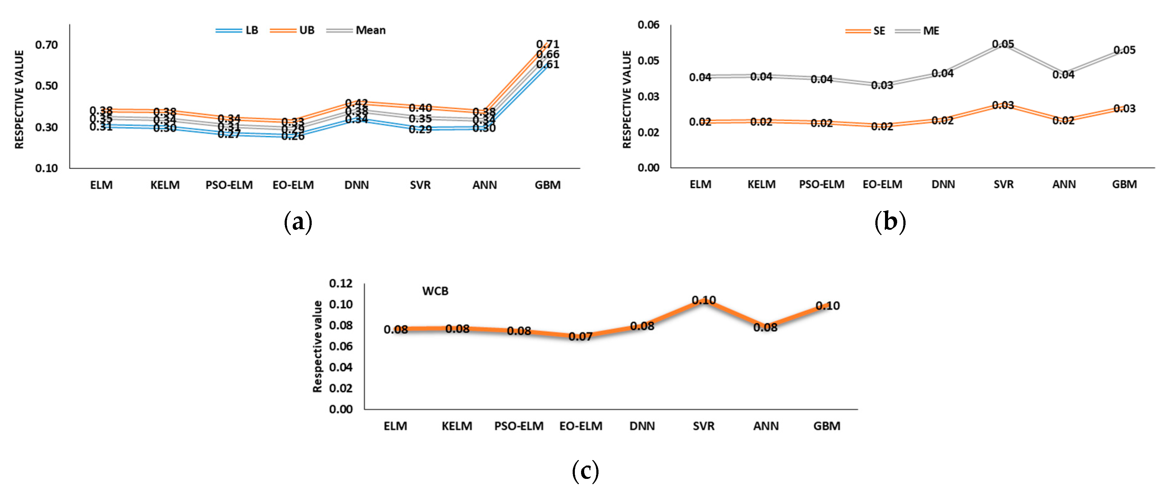
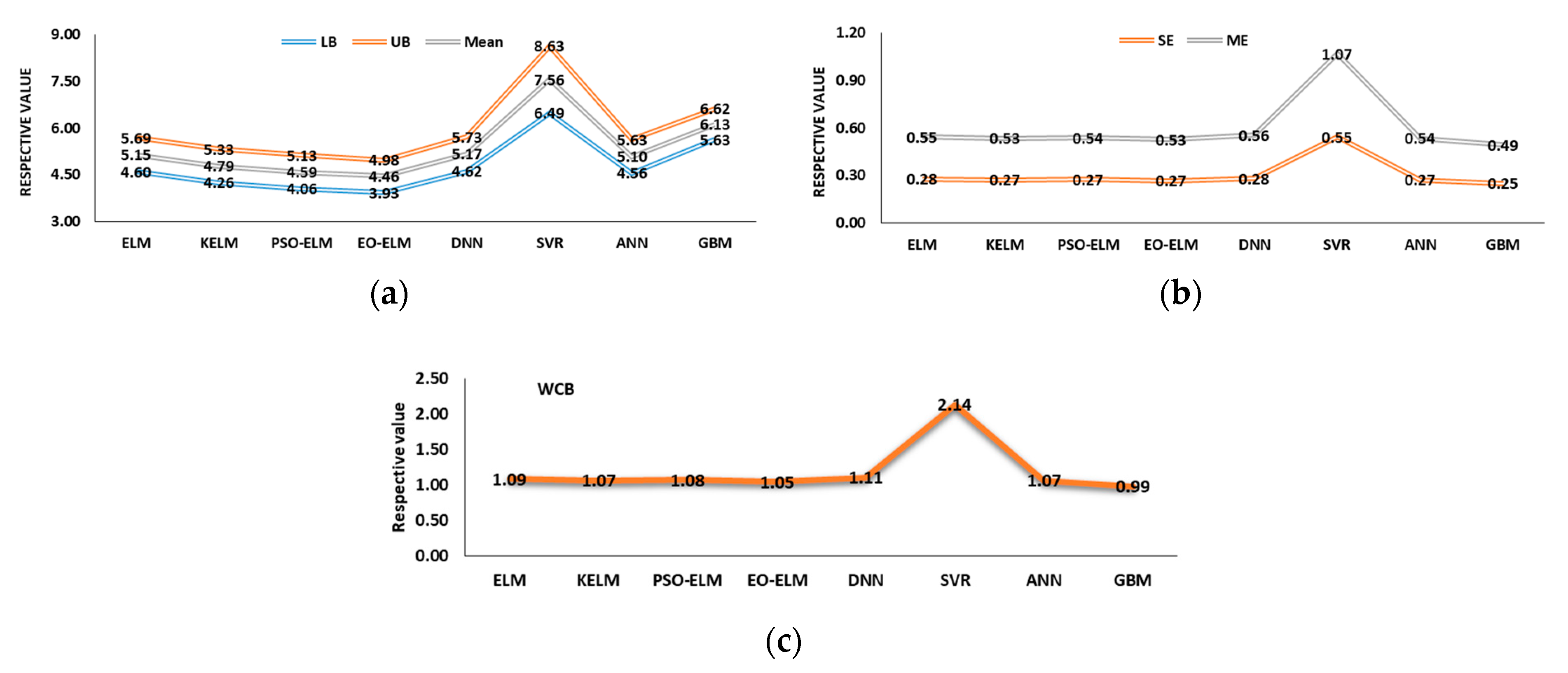
5.3.1. Lag-Based Models UA

The visualization of interrelationships of the uncertain variables between the lag-based models for both catchments is shown in Figure 20 (Fal at Tregony) and Figure 21 (Teifi at Glanteifi). Figure 20a–c and Figure 21a–c show the interrelationship of LB, UV and mean, SE and ME and WCB, respectively, for the models. For both catchments, LB, UV and mean (Figure 20a and Figure 21a) and SE (Figure 20b and Figure 21b) are lower for EO-ELM compared to other models. The ME (Figure 20b and Figure 21b) is almost similar for all models except SVR and GBM (lower compared to other). From UA, it is observed that WCB (Figure 20c and Figure 21c) also lower in EO-ELM. From UA, it is confirmed that EO-ELM has better prediction accuracy in the prediction runoff variable for both catchments.

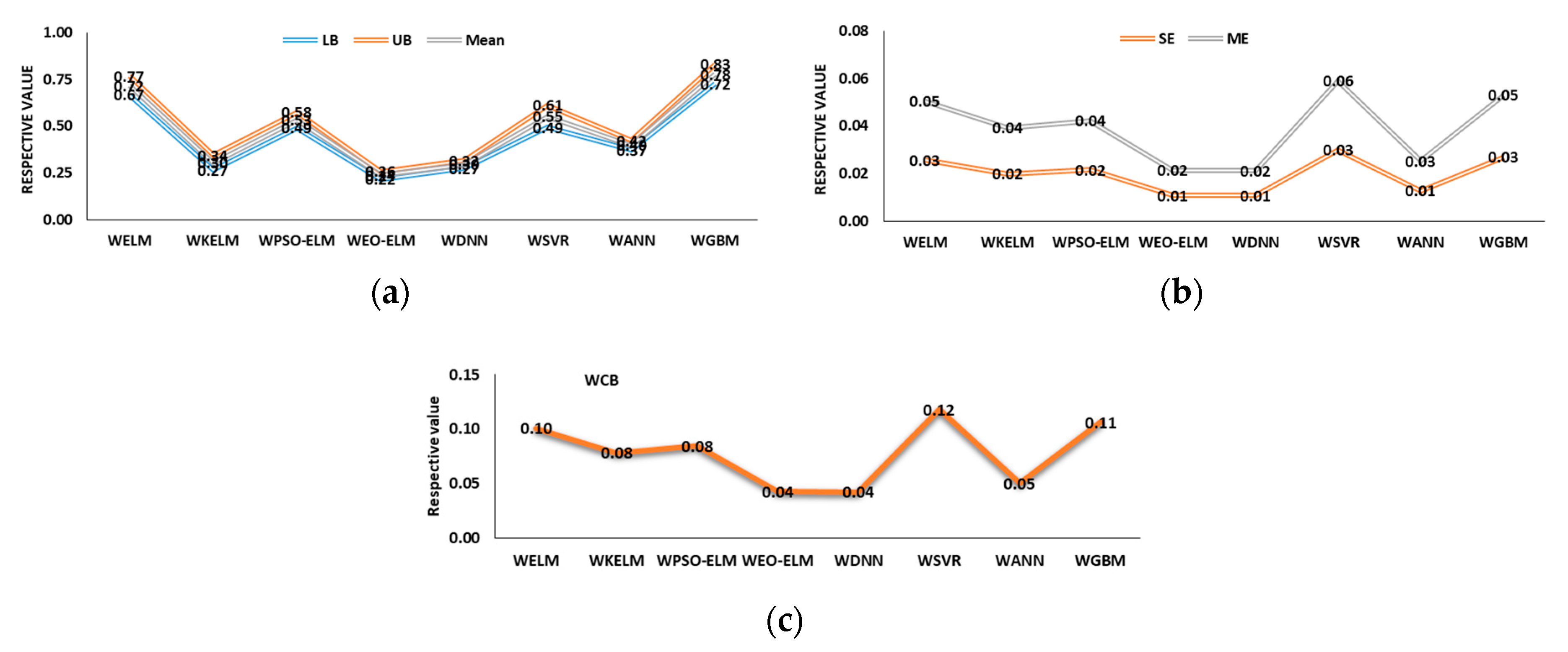
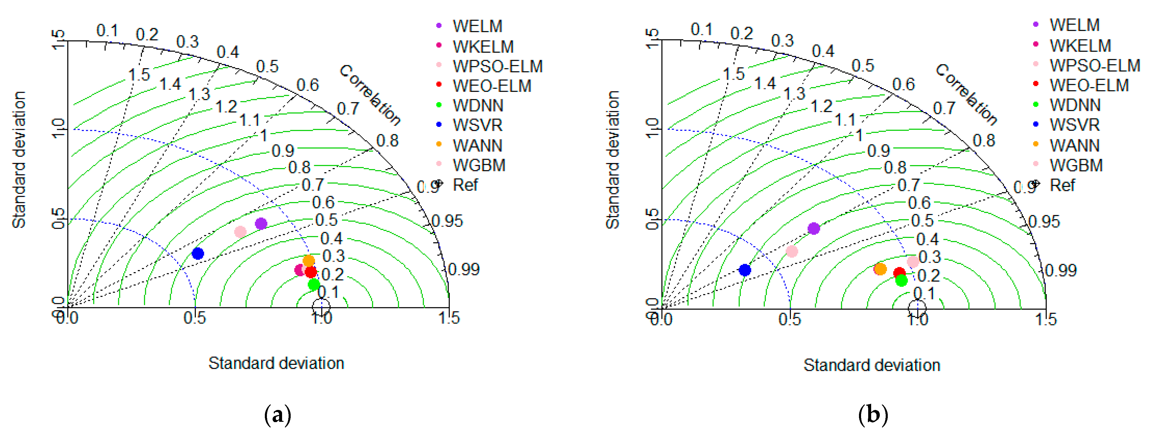
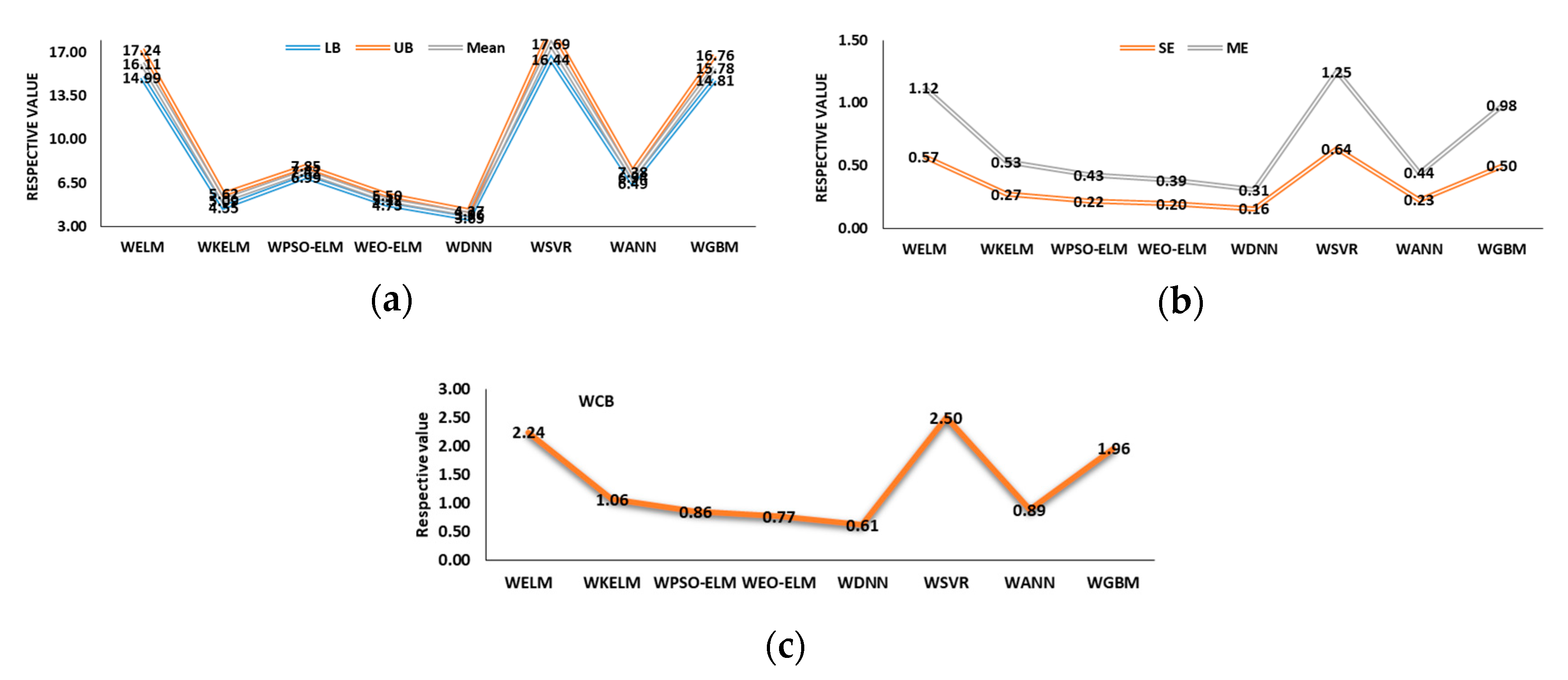
5.3.2. Wavelet-Based Models UA

The visualization of interrelationship of the variables between the wavelet-based models for both catchments is shown in Figure 22 (Fal at Tregony) and Figure 23 (Teifi at Glanteifi). Figure 22a–c and Figure 23a–c show the interrelationship of LB, UV and mean, SE and ME and WCB, respectively, for the models.

For catchment Fal at Tregony, LB, UV and mean (Figure 22a) and SE and ME (Figure 22b) are lower for WEO-ELM compared to other models. It can be observed that WCB (Figure 22c) also lower in WEO-ELM. WDNN is comparable with WEO-ELM in terms of SE and ME (Figure 22b) and WCB Figure 22c for Fal at Tregony. From UA, it is confirmed that WEO-ELM has better prediction accuracy in the prediction runoff variable along with WDNN for Fal at Tregony.

For the catchment of Teifi at Glanteifi, LB, UV and mean (Figure 23a) and SE and ME (Figure 23b) are lower for WDNN compared to other models. It can be observed that WCB (Figure 23c) is also lower in WDNN. The prediction accuracy of WEO-ELM follows WDNN and is better than the other six models for Teifi at Glanteifi. From UA, it is confirmed that WDNN has better prediction accuracy in prediction runoff variable for Teifi at Glanteifi.

5.4. Statistical Test: Two-Tailed t-Test

This study further investigates a statistical test, i.e., a two-tailed $t$-test that is used to determine if two sample means are equal [80]. This test is more suitable when the sample drawn from a population is sufficiently large (specifically more than 30), assuming that the data are normally distributed. In a two sample $t$-test, null hypothesis ($H_0$) indicates that the true mean difference between the paired is zero, i.e., ${\mu }_1-{\mu }_2=0$, while the alternate hypothesis ($H_A$) indicates that the true mean difference between the paired samples is not equal to zero, i.e., ${\mu }_1-{\mu }_2\ne 0$. Therefore, the procedure for implementing the two-tailed t-test is as follows:

$$\mathrm{Null}\mathrm{hypothesis}:H_0:{\mu }_1-{\mu }_2=0$$

(28)

$$\mathrm{Alternate}\mathrm{hypothesis}:H_A:{\mu }_1-{\mu }_2\ne 0$$

(29)

where ${\mu }_1$ and ${\mu }_1$ are the mean of two different samples. The test statistics can be calculated using the expression given by:

$$t_0=\frac{\left(\overline{x_1}-\overline{x_2}\right)-\left({\mu }_1-{\mu }_2\right)}{\sqrt{S_p^2\left(\frac{1}{n_1}+\frac{1}{n_2}\right)}}$$

(30)

where:

$$S_p^2=\frac{\left(n_1-1\right)S_1^2-\left(n_2-1\right)S_2^2}{n_1+n_2-2}$$

(31)

where $x_1$ and $x_2$ are the two observations under consideration, $n_1$ and $n_2$ are the total number of observations; $S_1$ and $S_2$ the standard deviation of two different samples, and $S_P$ is the pooled standard deviation. Calculated results at a significance level 5% (i.e., α = 0.05) assuming equal variances are presented in

Table 7. Two-tailed t-test for comparing models’ performance for Fal at Tragony.

Lag-Based	ELM	RBF-ELM	PSO-ELM	EOELM	DNN	SVM	ANN	GBM
Difference in mean abs. error	0.35	0.34	0.31	0.29	0.38	0.35	0.34	0.66
t Stat	0.04	0.29	0.42	1.43	1.02	2.46	0.56	−2.13
P(T ≤ t) two-tail	0.97	0.77	0.67	0.67	0.31	0.01	0.58	0.03
t Critical two-tail	1.96	1.96	1.96	1.96	1.96	1.96	1.96	1.96
Ho (accept if, |t Stat| < t Critical)	Accept	Accept	Accept	Accept	Accept	Reject	Accept	Accept
Wavelet-based	WELM	WRBF-ELM	WPSO-ELM	WEOELM	WDNN	SVM	ANN	WGBM
Difference in mean abs. error	0.72	0.30	0.53	0.29	0.30	0.55	0.40	0.78
t Stat	2.88	0.91	1.82	1.84	1.89	1.29	−0.22	1.44
P(T ≤ t) two-tail	0.00	0.36	0.07	0.92	0.14	0.20	0.82	0.15
t Critical two-tail	1.96	1.96	1.96	1.96	1.96	1.96	1.96	1.96
Ho (accept if, |t Stat| < t Critical)	Reject	Accept	Accept	Accept	Accept	Accept	Accept	Accept

and

Table 8. Two-tailed t-test for comparing models’ performance for Teifi at Glanteifi.

Lag-Based	ELM	RBF-ELM	PSO-ELM	EOELM	DNN	SVM	ANN	GBM
Difference in mean abs. error	5.15	4.79	4.59	4.46	5.17	7.56	5.10	6.13
t Stat	0.46	0.53	0.54	0.58	2.14	3.93	0.27	−0.35
P(T ≤ t) two-tail	0.65	0.60	0.59	0.56	0.03	0.00	0.79	0.73
t Critical two-tail	1.96	1.96	1.96	1.96	1.96	1.96	1.96	1.96
Ho (accept if, |t Stat| < t Critical)	Accept	Accept	Accept	Accept	Reject	Reject	Accept	Accept
Wavelet-based	WELM	WRBF-ELM	WPSO-ELM	WEOELM	WDNN	WSVM	WANN	WGBM
Difference in mean abs. error	16.11	5.09	7.42	4.12	3.96	17.69	6.94	15.78
t Stat	5.81	1.24	−1.51	1.11	1.57	0.86	0.02	1.39
P(T ≤ t) two-tail	0.00	0.21	0.13	0.55	0.79	0.39	0.98	0.16
t Critical two-tail	1.96	1.96	1.96	1.96	1.96	1.96	1.96	1.96
Ho (accept if, |t Stat| < t Critical)	Reject	Accept	Accept	Accept	Accept	Accept	Accept	Accept

for Fal at Tragony and Teifi at Glanteifi phases, respectively. Note that, the absolute values of $t$ Stat less than 1.96 (for the two-tailed test) indicate that there is no significant difference in mean between the samples. However, the obtained value closer to ideal value (i.e., $z_{0.025}$ = 1.96$\approx$|t stat|) indicates a more reliable model. As can be seen, the EO-ELM and WDNN satisfy the conditions in R-R modeling in Teifi at Glanteifi in the testing phase, while EO-ELM and WDNN satisfy the conditions in the Fal at Tragony testing phase.

From the above analysis, it may be concluded that the proposed EO-ELM is a better alternative integrated machine learning model with or without wavelet which gives better accuracy and generalization capability for R-R modeling in place of ELM, KELM, PSO-ELM, SVR, ANN, GBM and in UK. However, in the wavelet-based R-R modeling approach, WDNN performed better compared to other models. This was because increasing of the number of features in the dataset provides better efficacy in the proposed WDNN.

6. Conclusions

This paper developed two data-driven daily R-R modeling approaches, called EO-ELM and DNN, for two different benchmark stations of the catchment in the UK. The ELM, KELM, PSO-ANN, SVR, ANN, GBM were considered to validate the prediction performance of the proposed models. Initially, for an optimal number of input features, a PACF plot was used to feed the models. The main contributions of this paper are:

(i)

The use of a new metaheuristic algorithm (called EO) to optimize the input weights and hidden neuron biases of ELM are adequate for the better prediction performance by reducing the prediction error.

(ii)

The DWT is used to decompose the current day rainfall series (previous days rainfall series is already reflected in current day runoff series) and a runoff series (the highest correlated lag from PACF plot) to enhance the prediction performance of the proposed models (EO-ELM and DNN).

(iii)

Finally, the UA and two-tailed t-test confirm that EO-ELM performs best in optimal lag-based scenario and WDNN best for the wavelet-based scenario. WEO-ELM performs better compared to the other six models

For lag-based input, the experimental results showed that the one day-ahead discharge forecast performance of EO-ELM was better than the ELM, KELM, PSO-ELM, DNN, SVR, ANN, GBM. For wavelet-based input, the results showed that WDNN performed better due to enhancement of input features. However, WEO-ELM out-performed compared to WELM, WKELM, WPSO-ELM, WSVR, WANN and WGBM.

In future, the proposed model should be evaluated on other catchments’ data, and the performance of the other machine learning models should be compared to check the prediction capability of the proposed models. The proposed models can be applied to other time series hydrological variable predictions.

References

1. Wang, W.-C.; Chau, K.-W.; Cheng, C.-T.; Qiu, L. A comparison of performance of several artificial intelligence methods for forecasting monthly discharge time series. J. Hydrol. 2009, 374, 294–306. [Google Scholar] [CrossRef] [Green Version]
2. Salas, J.D. Applied Modeling of Hydrologic Time Series; Water Resources Publication: Littleton, CO, USA, 1980. [Google Scholar]
3. Awchi, T.A. River Discharges Forecasting In Northern Iraq Using Different ANN Techniques. Water Resour. Manag. 2014, 28, 801–814. [Google Scholar] [CrossRef]
4. Peng, Y.; Sun, X.; Zhang, X.; Zhou, H.; Zhang, Z. A Flood Forecasting Model that Considers the Impact of Hydraulic Projects by the Simulations of the Aggregate reservoir’s Retaining and Discharging. Water Resour. Manag. 2017, 31, 1031–1045. [Google Scholar] [CrossRef]
5. Ming, B.; Liu, P.; Bai, T.; Tang, R.; Feng, M. Improving Optimization Efficiency for Reservoir Operation Using a Search Space Reduction Method. Water Resour. Manag. 2017, 31, 1173–1190. [Google Scholar] [CrossRef]
6. Zhang, H.; Singh, V.P.; Wang, B.; Yu, Y. CEREF: A hybrid data-driven model for forecasting annual streamflow from a socio-hydrological system. J. Hydrol. 2016, 540, 246–256. [Google Scholar] [CrossRef]
7. Hrachowitz, M.; Savenije, H.; Bloschl, G.; Mcdonnell, J.; Sivapalan, M.; Pomeroy, J.; Arheimer, B.; Blume, T.; Clark, M.; Ehret, U.; et al. A decade of Predictions in Ungauged Basins (PUB)—A review. Hydrol. Sci. J. 2013, 58, 1198–1255. [Google Scholar] [CrossRef]
8. Mohammadi, K.; Eslami, H.; Kahawita, R. Parameter estimation of an ARMA model for river flow forecasting using goal programming. J. Hydrol. 2006, 331, 293–299. [Google Scholar] [CrossRef]
9. Mehdizadeh, S.; Fathian, F.; Adamowski, J.F. Hybrid artificial intelligence-time series models for monthly streamflow modeling. Appl. Soft Comput. 2019, 80, 873–887. [Google Scholar] [CrossRef]
10. Nayak, P.; Sudheer, K.; Rangan, D.; Ramasastri, K. A neuro-fuzzy computing technique for modeling hydrological time series. J. Hydrol. 2004, 291, 52–66. [Google Scholar] [CrossRef]
11. Bui, Y.T.; Orange, D.; Visser, S.; Hoanh, C.T.; Laissus, M.; Poortinga, A.; Tran, D.T.; Stroosnijder, L. Lumped surface and sub--surface runoff for erosion modeling within a small hilly watershed in northern Vietnam. Hydrol. Process. 2014, 28, 2961–2974. [Google Scholar] [CrossRef]
12. Beven, J.K. Rainfall-Runoff Modelling: The Primer; John Willey & Sons Ltd.: New York, NY, USA, 2000. [Google Scholar]
13. Liu, Z.; Todini, E. Towards a comprehensive physically-based rainfall-runoff model. Hydrol. Earth Syst. Sci. 2002, 6, 859–881. [Google Scholar] [CrossRef]
14. Modarres, R.; Ouarda, T. Modeling rainfall–runoff relationship using multivariate GARCH model. J. Hydrol. 2013, 499, 1–18. [Google Scholar] [CrossRef]
15. Samsudin, R.A.; Saad, P.; Shabri, A. River flow time series using least squares support vector machines. Hydrol. Earth Syst. Sci. 2011, 15, 1835–1852. [Google Scholar] [CrossRef] [Green Version]
16. Wu, C.; Chau, K.W. Rainfall–runoff modeling using artificial neural network coupled with singular spectrum analysis. J. Hydrol. 2011, 399, 394–409. [Google Scholar] [CrossRef] [Green Version]
17. Lolli, F.; Gamberini, R.; Regattieri, A.; Balugani, E.; Gatos, T.; Gucci, S. Single-hidden layer neural networks for forecasting intermittent demand. Int. J. Prod. Econ. 2017, 183, 116–128. [Google Scholar] [CrossRef]
18. Nourani, V. An Emotional ANN (EANN) approach to modeling rainfall-runoff process. J. Hydrol. 2017, 544, 267–277. [Google Scholar] [CrossRef]
19. Motahari, M.; Mazandaranizadeh, H. Development of a PSO-ANN Model for Rainfall-Runoff Response in Basins, Case Study: Karaj Basin. Civ. Eng. J. 2017, 3, 35–44. [Google Scholar] [CrossRef]
20. Taormina, R.; Chau, K.-W. Neural network river forecasting with multi-objective fully informed particle swarm optimization. J. Hydroinform. 2015, 17, 99–113. [Google Scholar] [CrossRef] [Green Version]
21. Huang, G.-B. An Insight into Extreme Learning Machines: Random Neurons, Random Features and Kernels. Cogn. Comput. 2014, 6, 376–390. [Google Scholar] [CrossRef]
22. Rezaie-Balf, M.; Kisi, O. New formulation for forecasting streamflow: Evolutionary polynomial regression vs. extreme learning machine. Hydrol. Res. 2018, 49, 939–953. [Google Scholar] [CrossRef] [Green Version]
23. Yaseen, Z.M.; Jaafar, O.; Deo, R.C.; Kisi, O.; Adamowski, J.; Quilty, J.; El-Shafie, A. Stream-flow forecasting using extreme learning machines: A case study in a semi-arid region in Iraq. J. Hydrol. 2016, 542, 603–614. [Google Scholar] [CrossRef]
24. Zhu, S.; Heddam, S.; Wu, S.; Dai, J.; Jia, B. Extreme learning machine-based prediction of daily water temperature for rivers. Environ. Earth Sci. 2019, 78, 202. [Google Scholar] [CrossRef]
25. Deo, R.C.; Tiwari, M.K.; Adamowski, J.F.; Quilty, J. Forecasting effective drought index using a wavelet extreme learning machine (W-ELM) model. Stoch. Environ. Res. Risk Assess. 2017, 31, 1211–1240. [Google Scholar] [CrossRef]
26. Fijani, E.; Barzegar, R.; Deo, R.; Tziritis, E.; Skordas, K. Design and implementation of a hybrid model based on two-layer decomposition method coupled with extreme learning machines to support real-time environmental monitoring of water quality parameters. Sci. Total Environ. 2019, 648, 839–853. [Google Scholar] [CrossRef] [PubMed]
27. Cao, J.; Lin, Z.; Huang, G.-B. Self-Adaptive Evolutionary Extreme Learning Machine. Neural Process. Lett. 2012, 36, 285–305. [Google Scholar] [CrossRef]
28. Zhu, Q.-Y.; Qin, K.; Suganthan, P.; Huang, G.-B. Evolutionary extreme learning machine. Pattern Recognit. 2005, 38, 1759–1763. [Google Scholar] [CrossRef]
29. Huang, G.; Huang, G.B.; Song, S.; You, K. Trends in extreme learning machines: A review. Neural Netw. 2015, 61, 32–48. [Google Scholar] [CrossRef] [PubMed]
30. Roy, B.; Singh, M.P.; Singh, A. A novel approach for rainfall-runoff modelling using a biogeography-based optimization technique. Int. J. River Basin Manag. 2019, 19, 1–14. [Google Scholar] [CrossRef]
31. Chau, K. Particle swarm optimization training algorithm for ANNs in stage prediction of Shing Mun River. J. Hydrol. 2006, 329, 363–367. [Google Scholar] [CrossRef] [Green Version]
32. Stagge, J.H.; Moglen, G.E. Evolutionary Algorithm Optimization of a Multireservoir System with Long Lag Times. J. Hydrol. Eng. 2014, 19, 05014011. [Google Scholar] [CrossRef]
33. Li, P.; Chen, B.; Li, Z.L.; Jing, L. ASOC: A Novel Agent-Based Simulation-Optimization Coupling Approach-Algorithm and Application in Offshore Oil Spill Responses. J. Environ. Inform. 2016, 28, 90–100. [Google Scholar] [CrossRef]
34. Yi, L.; Zhao, J.; Yu, W.; Liu, Y.; Yi, C.; Jiang, D. Catenary Fault Identification Based on PSO-ELM. J. Phys. Conf. Ser. 2019, 1302, 032017. [Google Scholar] [CrossRef] [Green Version]
35. Cai, W.; Yang, J.; Yu, Y.; Song, Y.; Zhou, T.; Qin, J. PSO-ELM: A Hybrid Learning Model for Short-Term Traffic Flow Forecasting. IEEE Access 2020, 8, 6505–6514. [Google Scholar] [CrossRef]
36. Kaloop, M.R.; Kumar, D.; Samui, P.; Gabr, A.R.; Hu, J.W.; Jin, X.; Roy, B. Particle Swarm Optimization Algorithm-Extreme Learning Machine (PSO-ELM) Model for Predicting Resilient Modulus of Stabilized Aggregate Bases. Appl. Sci. 2019, 9, 3221. [Google Scholar] [CrossRef] [Green Version]
37. Murlidhar, B.R.; Kumar, D.; Armaghani, D.J.; Mohamad, E.T.; Roy, B.; Pham, B.T. A Novel Intelligent ELM-BBO Technique for Predicting Distance of Mine Blasting-Induced Flyrock. Nat. Resour. Res. 2020, 29, 4103–4120. [Google Scholar] [CrossRef]
38. Armaghani, D.J.; Kumar, D.; Samui, P.; Hasanipanah, M.; Roy, B. A novel approach for forecasting of ground vibrations resulting from blasting: Modified particle swarm optimization coupled extreme learning machine. Eng. Comput. 2020, 1–15. [Google Scholar] [CrossRef]
39. Faramarzi, A.; Heidarinejad, M.; Stephens, B.; Mirjalili, S. Equilibrium optimizer: A novel optimization algorithm. Knowl. Based Syst. 2020, 191, 105190. [Google Scholar] [CrossRef]
40. Bengio, Y. Learning Deep Architectures for AI. Found. Trends Mach. Learn. 2009, 2, 1–127. [Google Scholar] [CrossRef]
41. Collobert, R.; Weston, J.; Bottou, L.; Karlen, M.; Kavukcuoglu, K.; Kuksa, P. Natural language processing (almost) from scratch. J. Mach. Learn. Res. 2011, 12, 2493–2537. [Google Scholar]
42. Mikolov, T.; Deoras, A.; Povey, D.; Burget, L.; Cernocky, J. Strategies for training large scale neural network language models. In 2011 IEEE Workshop on Automatic Speech Recognition & Understanding; IEEE: Piscataway, NJ, USA, 2011. [Google Scholar]
43. Arel, I.; Rose, D.C.; Karnowski, T.P. Deep Machine Learning-A New Frontier in Artificial Intelligence Research [Research Frontier]. IEEE Comput. Intell. Mag. 2010, 5, 13–18. [Google Scholar] [CrossRef]
44. Krizhevsky, A.; Sutskever, I.; Hinton, G.E. Imagenet classification with deep convolutional neural networks. Commun. ACM 2017, 60, 84–90. [Google Scholar] [CrossRef]
45. Längkvist, M.; Karlsson, L.; Loutfi, A. A review of unsupervised feature learning and deep learning for time-series modeling. Pattern Recognit. Lett. 2014, 42, 11–24. [Google Scholar] [CrossRef] [Green Version]
46. Harrigan, S.; Hannaford, J.; Muchan, K.; Marsh, T.J. Designation and trend analysis of the updated UK Benchmark Network of river flow stations: The UKBN2 dataset. Hydrol. Res. 2018, 49, 552–567. [Google Scholar] [CrossRef] [Green Version]
47. Mouatadid, S.; Adamowski, J.F.; Tiwari, M.K.; Quilty, J.M. Coupling the maximum overlap discrete wavelet transform and long short-term memory networks for irrigation flow forecasting. Agric. Water Manag. 2019, 219, 72–85. [Google Scholar] [CrossRef]
48. Rhif, M.; Ben Abbes, A.; Farah, I.R.; Martínez, B.; Sang, Y. Wavelet Transform Application for/in Non-Stationary Time-Series Analysis: A Review. Appl. Sci. 2019, 9, 1345. [Google Scholar] [CrossRef] [Green Version]
49. Sun, Y.; Niu, J.; Sivakumar, B. A comparative study of models for short-term streamflow forecasting with emphasis on wavelet-based approach. Stoch. Environ. Res. Risk Assess. 2019, 33, 1875–1891. [Google Scholar] [CrossRef]
50. Altunkaynak, A.; Nigussie, T.A. Prediction of daily rainfall by a hybrid wavelet-season-neuro technique. J. Hydrol. 2015, 529, 287–301. [Google Scholar] [CrossRef]
51. Niu, J.; Chen, J.; Wang, K.; Sivakumar, B. Multi-scale streamflow variability responses to precipitation over the headwater catchments in southern China. J. Hydrol. 2017, 551, 14–28. [Google Scholar] [CrossRef]
52. Chong, K.L.; Lai, S.H.; El-Shafie, A. Wavelet Transform Based Method for River Stream Flow Time Series Frequency Analysis and Assessment in Tropical Environment. Water Resour. Manag. 2019, 33, 2015–2032. [Google Scholar] [CrossRef]
53. Yong, N.K.; Awang, N. Wavelet-based time series model to improve the forecast accuracy of PM10 concentrations in Peninsular Malaysia. Environ. Monit. Assess. 2019, 191, 64. [Google Scholar] [CrossRef]
54. Graf, R.; Zhu, S.; Sivakumar, B. Forecasting river water temperature time series using a wavelet–neural network hybrid modelling approach. J. Hydrol. 2019, 578, 124115. [Google Scholar] [CrossRef]
55. Chen, L.; Hao, Y.; Hu, X. Detection of preterm birth in electrohysterogram signals based on wavelet transform and stacked sparse autoencoder. PLoS ONE 2019, 14, e0214712. [Google Scholar] [CrossRef] [PubMed]
56. Farboudfam, N.; Nourani, V.; Aminnejad, B. Wavelet-based multi station disaggregation of rainfall time series in mountainous regions. Hydrol. Res. 2019, 50, 545–561. [Google Scholar] [CrossRef] [Green Version]
57. Kennedy, J.; Eberhart, R. Particle swarm optimization (PSO). In Proceedings of the IEEE International Conference on Neural Networks, Perth, Australia, 27 November–1 December 1995. [Google Scholar]
58. Kisi, O.; Cimen, M. Precipitation forecasting by using wavelet-support vector machine conjunction model. Eng. Appl. Artif. Intell. 2012, 25, 783–792. [Google Scholar] [CrossRef]
59. Labat, D.; Ronchail, J.; Guyot, J.L. Recent advances in wavelet analyses: Part 2—Amazon, Parana, Orinoco and Congo discharges time scale variability. J. Hydrol. 2005, 314, 289–311. [Google Scholar] [CrossRef]
60. Wang, W.; Ding, J. Wavelet network model and its application to the prediction of hydrology. Nat. Sci. 2003, 1, 67–71. [Google Scholar]
61. Jiang, S.; Xiao, R.; Wang, L.; Luo, X.; Huang, C.; Wang, J.-H.; Chin, K.-S.; Nie, X. Combining Deep Neural Networks and Classical Time Series Regression Models for Forecasting Patient Flows in Hong Kong. IEEE Access 2019, 7, 118965–118974. [Google Scholar] [CrossRef]
62. Huang, G.-B.; Zhu, Q.-Y.; Siew, C.-K. Extreme learning machine: Theory and applications. Neurocomputing 2006, 70, 489–501. [Google Scholar] [CrossRef]
63. Huang, G.-B.; Zhou, H.; Ding, X.; Zhang, R. Extreme Learning Machine for Regression and Multiclass Classification. IEEE Trans. Syst. Man Cybern. Part B (Cybern.) 2012, 42, 513–529. [Google Scholar] [CrossRef] [Green Version]
64. Huang, G.-B.; Wang, D.H.; Lan, Y. Extreme learning machines: A survey. Int. J. Mach. Learn. Cybern. 2011, 2, 107–122. [Google Scholar] [CrossRef]
65. Huang, G.-B.; Siew, C.-K. Extreme learning machine: RBF network case. In Proceedings of the ICARCV 2004 8th Control, Automation, Robotics and Vision Conference, Kunming, China, 6–9 December 2004; IEEE: Piscataway, NJ, USA, 2004. [Google Scholar]
66. Drucker, H.; Burges, C.J.; Kaufman, L.; Smola, A.J.; Vapnik, V. Support vector regression machines. Adv. Neural Inf. Process. Syst. 1997, 9, 155–161. [Google Scholar]
67. Maheswaran, R.; Khosa, R. Comparative study of different wavelets for hydrologic forecasting. Comput. Geosci. 2012, 46, 284–295. [Google Scholar] [CrossRef]
68. Gold, C.M. Surface interpolation, spatial adjacency and GIS. In Three Dimensional Applications in Geographic Information Systems; CRC Press: Boca Raton, FL, USA, 1989; pp. 21–35. [Google Scholar]
69. Touzani, S.; Granderson, J.; Fernandes, S. Gradient boosting machine for modeling the energy consumption of commercial buildings. Energy Build. 2018, 158, 1533–1543. [Google Scholar] [CrossRef] [Green Version]
70. Robinson, E.L.; Blyth, E.M.; Clark, D.B.; Finch, J.; Rudd, A.C. Trends in atmospheric evaporative demand in Great Britain using high-resolution meteorological data. Hydrol. Earth Syst. Sci. 2017, 21, 1189–1224. [Google Scholar] [CrossRef] [Green Version]
71. Keller, V.; Tanguy, M.; Prosdocimi, I.; Terry, J.A.; Hitt, O.; Cole, S.J.; Fry, M.; Morris, D.G.; Dixon, H. CEH-GEAR: 1 km resolution daily and monthly areal rainfall estimates for the UK for hydrological and other applications. Earth Syst. Sci. Data 2015, 7, 143–155. [Google Scholar] [CrossRef] [Green Version]
72. Tanguy, M.; Dixon, H.; Prosdocimi, I.; Morris, D.G.; Keller, V.D.J. Gridded Estimates of Daily and Monthly Areal Rainfall for the United Kingdom (1890–2015) [CEH-GEAR]; NERC Environmental Information Data Centre: Atlanta, GA, USA, 2016. [Google Scholar]
73. Kumar, R.; Singh, M.P.; Roy, B.; Shahid, A.H. A Comparative Assessment of Metaheuristic Optimized Extreme Learning Machine and Deep Neural Network in Multi-Step-Ahead Long-term Rainfall Prediction for All-Indian Regions. Water Resour. Manag. 2021, 35, 1927–1960. [Google Scholar] [CrossRef]
74. De Artigas, M.Z.; Elias, A.G.; de Campra, P.F. Discrete wavelet analysis to assess long-term trends in geomagnetic activity. Phys. Chem. Earth Parts A/B/C 2006, 31, 77–80. [Google Scholar] [CrossRef]
75. Bigiarini, M.Z.; Bigiarini, M.M.Z. Package “hydroGOF”. R-Package. 2013. Available online: www.r-project.org/ (accessed on 7 May 2018).
76. Gholami, A.; Bonakdari, H.; Samui, P.; Mohammadian, M.; Gharabaghi, B. Predicting stable alluvial channel profiles using emotional artificial neural networks. Appl. Soft Comput. 2019, 78, 420–437. [Google Scholar] [CrossRef]
77. Zeng, J.; Roy, B.; Kumar, D.; Mohammed, A.S.; Armaghani, D.J.; Zhou, J.; Mohamad, E.T. Proposing several hybrid PSO-extreme learning machine techniques to predict TBM performance. Eng. Comput. 2021, 1–17. [Google Scholar] [CrossRef]
78. Roy, B.; Singh, M.P. An empirical-based rainfall-runoff modelling using optimization technique. Int. J. River Basin Manag. 2019, 18, 49–67. [Google Scholar] [CrossRef]
79. Roy, B.; Singh, M.P. A Metaheuristic-based Emotional ANN (EmNN) Approach for Rainfall-runoff Modeling. In Proceedings of the 2019 International Conference on Communication and Electronics Systems (ICCES), Coimbatore, India, 17–19 July 2019; pp. 454–458. [Google Scholar] [CrossRef]
80. Kardani, N.; Bardhan, A.; Kim, D.; Samui, P.; Zhou, A. Modelling the energy performance of residential buildings using advanced computational frameworks based on RVM, GMDH, ANFIS-BBO and ANFIS-IPSO. J. Build. Eng. 2021, 35, 102105. [Google Scholar] [CrossRef]
Figure 1. Architecture of a deep neural network (DNN) for runoff prediction.
Applsci 11 06238 g001
Figure 2. Single hidden layer neural connection.
Applsci 11 06238 g002
Figure 3. Daily discharge and rainfall of (a) the small basin (Fal at Tregony), (b) the large basin (Teifi at Glanteifi).
Applsci 11 06238 g003
Figure 4. Process flow chart of the deep neural network (DNN).
Applsci 11 06238 g004
Figure 5. Autocorrelation function (ACF) and partial autocorrelation function (PACF) plots for daily discharge data of catchment Fal at Tregony (a,b) and Teifi at Glanteifi (c,d), respectively.
Applsci 11 06238 g005
Figure 6. Discrete wavelet transform (DWT) sub-series (D1 to D9) and approximation (A9) for Teifi at Glanteifi (a) discharge (b) rainfall and Fal at Tregony (c) discharge (d) rainfall.
Applsci 11 06238 g006aApplsci 11 06238 g006b
Figure 7. Prediction capability of the eight models in train case (a) ELM, (b) KELM, (c) PSO-ELM, (d) EO-ELM, (e) DNN, (f) SVR, (g) ANN, and (h) GBM for the catchment Fal at Tregony.
Applsci 11 06238 g007
Figure 8. Prediction capability of the eight models in test case (a) ELM, (b) KELM, (c) PSO-ELM, (d) EO-ELM, (e) DNN, (f) SVR, (g) ANN, and (h) GBM for the catchment Fal at Tregony.
Applsci 11 06238 g008
Figure 9. Test case observe vs. predicted runoff of (a) EO-ELM and (b) PSO-ELM for catchment Fal at Tregony.
Applsci 11 06238 g009
Figure 10. Statistical comparison for all models for catchment Fal at Tregony: (a) train, (b) test.
Applsci 11 06238 g010aApplsci 11 06238 g010b
Figure 11. Prediction capability of the eight models in train case (a) ELM, (b) KELM, (c) PSO-ELM, (d) EO-ELM, (e) DNN, (f) SVR, (g) ANN, and (h) GBM for the catchment Teifi at Glanteifi.
Applsci 11 06238 g011
Figure 12. Prediction capability of the eight models in test case (a) ELM, (b) KELM, (c) PSO-ELM, (d) EO-ELM, (e) DNN, (f) SVR, (g) ANN, and (h) GBM for the catchment Teifi at Glanteifi.
Applsci 11 06238 g012
Figure 13. Statistical comparison for all models for catchment Teifi at Glanteifi: (a) train and (b) test.
Applsci 11 06238 g013aApplsci 11 06238 g013b
Figure 14. Prediction capability of the eight models in train case (a) WELM, (b) WKELM, (c) WPSO-ELM, (d) WEO-ELM, (e) WDNN, (f) WSVR, (g) WANN, and (h) WGBM for the catchment Fal at Tregony.
Applsci 11 06238 g014
Figure 15. Prediction capability of the eight models in test case (a) WELM, (b) WKELM, (c) WPSO-ELM, (d) WEO-ELM, (e) WDNN, (f) WSVR, (g) WANN, and (h) WGBM for the catchment Fal at Tregony.
Applsci 11 06238 g015
Figure 16. Statistical comparison for all models for catchment Fal at Tregony: (a) Train, and (b) Test.
Applsci 11 06238 g016
Figure 17. Prediction capability of the eight models in train case (a) WELM, (b) WKELM, (c) WPSO-ELM, (d) WEO-ELM, (e) WDNN, (f) WSVR, (g) WANN, and (h) WGBM for the catchment Teifi at Glanteifi.
Applsci 11 06238 g017
Figure 18. Prediction capability of the eight models in test case (a) WELM, (b) WKELM, (c) WPSO-ELM, (d) WEO-ELM, (e) WDNN, (f) WSVR, (g) WANN, and (h) WGBM for the catchment Teifi at Glanteifi.
Applsci 11 06238 g018
Figure 19. Statistical comparison for all models for catchment Teifi at Glanteifi: (a) train, and (b) test.
Applsci 11 06238 g019
Figure 20. Visual representation of UA for lag-based models (Fal at Tregony), (a) lower bound (LB), upper bound (UB) and mean; (b) standard error (SE) and margin of error (ME); (c) WCB.
Applsci 11 06238 g020
Figure 21. Visual representation of uncertainty analysis (UA) for lag-based models (Teifi at Glanteifi), (a) LB, UB and Mean; (b) SE and ME; (c) width of confidence (WCB).
Applsci 11 06238 g021
Figure 22. Visual representation of UA for wavelet-based models (Fal at Tregony), (a) LB, UB and Mean; (b) SE and ME; (c) WCB.
Applsci 11 06238 g022
Figure 23. Visual representation of UA for wavelet-based models (Teifi at Glanteifi), (a) LB, UB and Mean; (b) SE and ME; (c) WCB.
Applsci 11 06238 g023