Article

Real-Time AI-Based Informational Decision-Making Support System Utilizing Dynamic Text Sources

Department of Electrical and Computer Engineering, Inha University, Incheon 22212, Korea
*
Author to whom correspondence should be addressed.
Appl. Sci. 2021, 11(13), 6237; https://doi.org/10.3390/app11136237
Submission received: 7 May 2021 / Revised: 24 June 2021 / Accepted: 25 June 2021 / Published: 5 July 2021
(This article belongs to the Special Issue Deep Convolutional Neural Networks)

Abstract

:
Unstructured data from the internet constitute large sources of information, which need to be formatted in a user-friendly way. This research develops a model that classifies unstructured data from data mining into labeled data, and builds an informational and decision-making support system (DMSS). We often have assortments of information collected by mining data from various sources, where the key challenge is to extract valuable information. We observe substantial classification accuracy enhancement for our datasets with both machine learning and deep learning algorithms. The highest classification accuracy (99% in training, 96% in testing) was achieved from a Covid corpus which is processed by using a long short-term memory (LSTM). Furthermore, we conducted tests on large datasets relevant to the Disaster corpus, with an LSTM classification accuracy of 98%. In addition, random forest (RF), a machine learning algorithm, provides a reasonable 84% accuracy. This research’s main objective is to increase the application’s robustness by integrating intelligence into the developed DMSS, which provides insight into the user’s intent, despite dealing with a noisy dataset. Our designed model selects the random forest and stochastic gradient descent (SGD) algorithms’ F1 score, where the RF method outperforms by improving accuracy by 2% (to 83% from 81%) compared with a conventional method.

1. Introduction

Information mining is a cycle that finds relevant patterns from a large amount of data. After collecting these data, text classification (which depends on the content and which dynamically classifies many texts from different fields on the internet) builds an innovative system, relationship, and decision through natural language processing (NLP) [1]. Clustering, classification, information extraction, and information mining include various text preparation steps needing powerful data models because of inconsistencies and non-standard noise in digitized messages. In NLP, text arrangement is considered difficult because of the different types of information representation [2].
Social media data mining is used to uncover hidden patterns and trends from social media network (SMN) platforms like Twitter, LinkedIn, Facebook, and others [3]. There is unstructured content on social media—like tweets, comments, status updates—which is not only based on businesses, firms, and agencies but also have Public Protection Disaster Relief (PPDR) and DMSS-related information [3].
De Oliveira et al. [4] mention anonymous real-time data to generate information which allows sentiment analysis on a given subject and Gajjala et al. [5] cite classification for sentiment analysis. Damaschk et al. [6] analyzed multiclass text classification on noisy data. To improve the performance of DSS, Wang et al. [7] used intelligent techniques for traffic prediction and Balbo and Pinson [8] applied intelligent agents for transportation management. Learning methods includes supervised and unsupervised methods, Tzima and Mitkas [9] for rule extraction, Herrero et al. [10] for traffic risk analysis, and Yu et al. [11] for traffic prediction. Zarei et al. [12] also investigated the effects of learning methods in DSS based on historical data. Shadi et al. [13] quote supervised and unsupervised learning decision support systems for incident management in an intelligent tunnel. Most of the research work examines only particular disasters or specific event analysis based on existing or scraping datasets, but comparative research on a decision support system that gives reliable information has not been extensively applied during a large or diverse set of crises. Aiming to provide real-time information for DMSS, this research provides data collecting and proposed methods for data cleaning and grouping, sentiment analysis, topic labeling for data categorization, chatbot application for sentence-based decision-making, unknown sentence prediction and decision, and finally DMSS from data visualization. Our novelty of this work is divergent from others because the model arranges user’s statements regarding the real-time situational information from any large or short corpus which encourages them to make an event analysis, visualization, informational data support by a chatbot, and DMSS. In addition, we experimented with short corpus data which gives informed decisions based on its authenticity. If the model gives an informational decision within a short dataset, it can provide also good accuracy and decisions among the larger ones. For this reason, we did evaluations with both short corpus (unsupervised) and larger corpus (supervised) chatbot in 
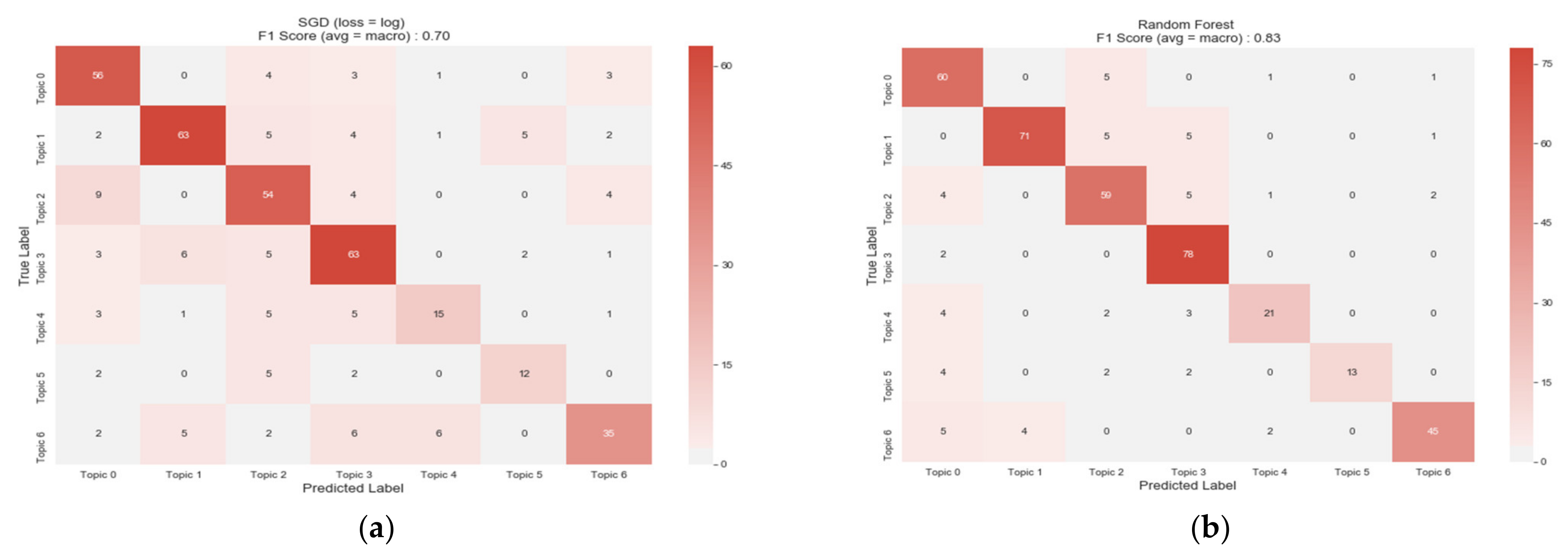
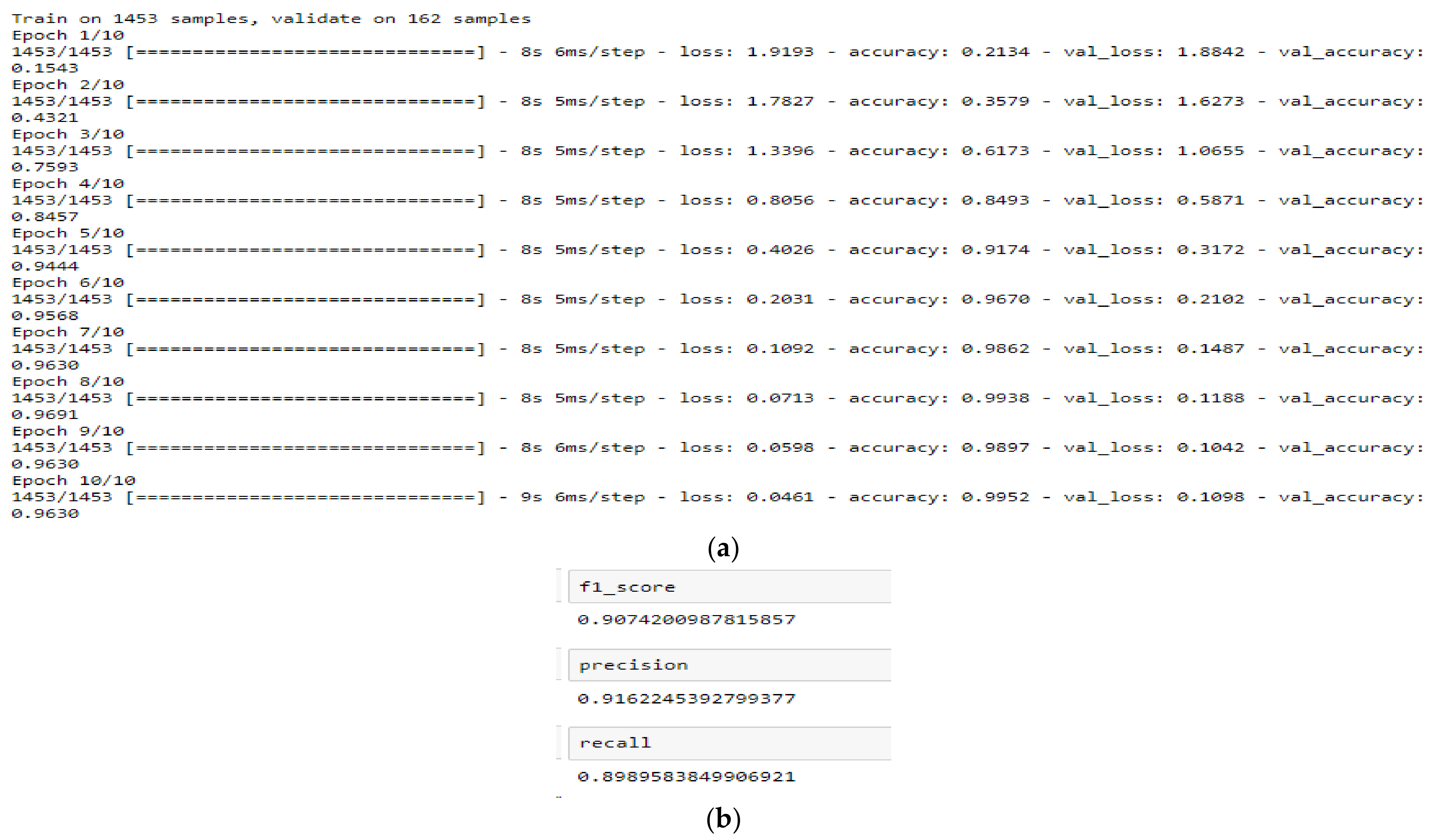
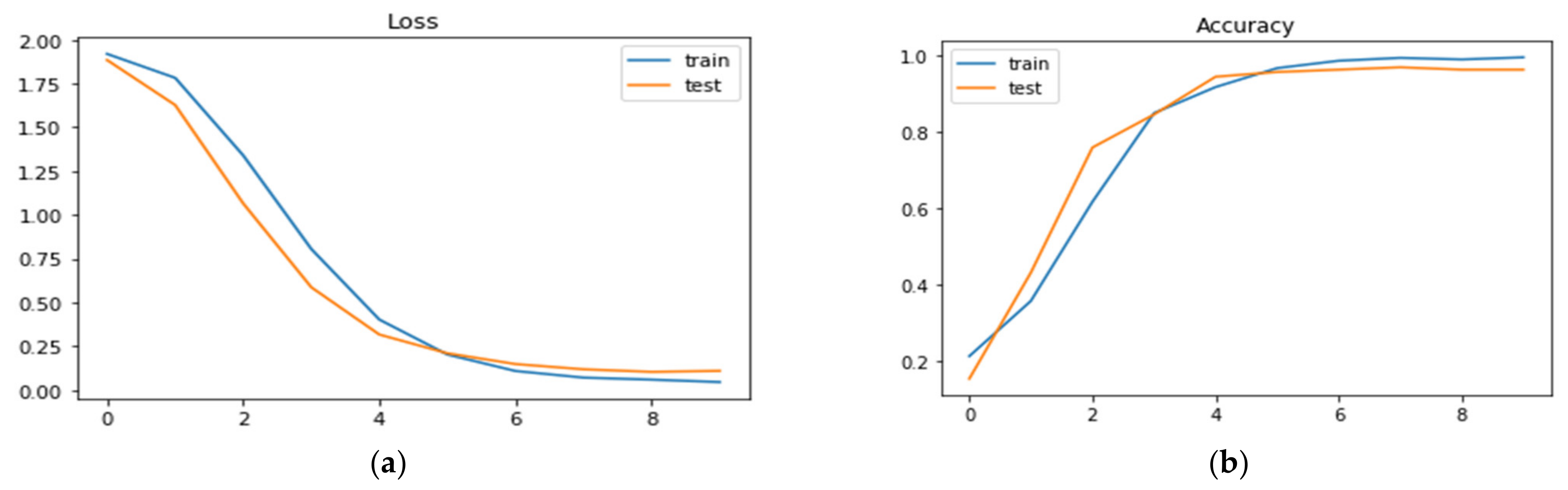
Section 6 and shows their sentence accuracy label which is both cases (>98%). We achieved 96% and 99% accuracy in test and training datasets by using LSTM on a short corpus in the DL method. Moreover, the ML method using hyper-parameter in the dataset, a random forest algorithm increases data accuracy in the F1 score which is 2% (81–83%).
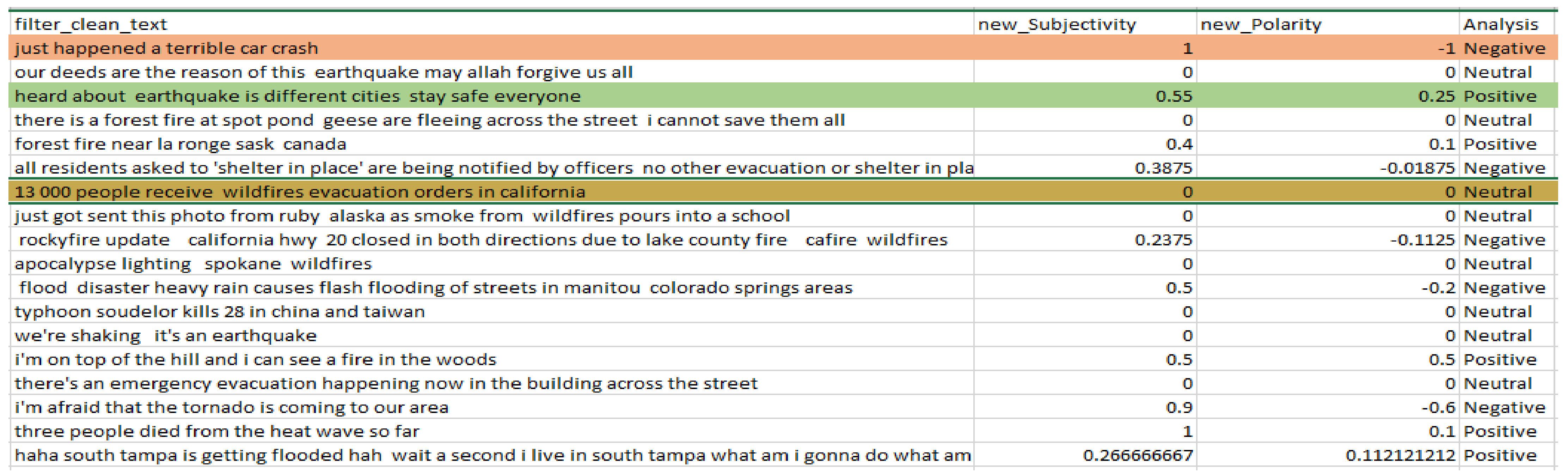
We used a completely different dataset for model verification, which is the Disaster corpus. The previous corpus contained 1635 sentences, whereas this corpus contains 10,875 sentences. Surprisingly, the data behavior that is employed in decision-making appears to be comparable in both circumstances. Furthermore, the deep learning LSTM model has an accuracy of over 98% in both Disaster and Covid scenarios.
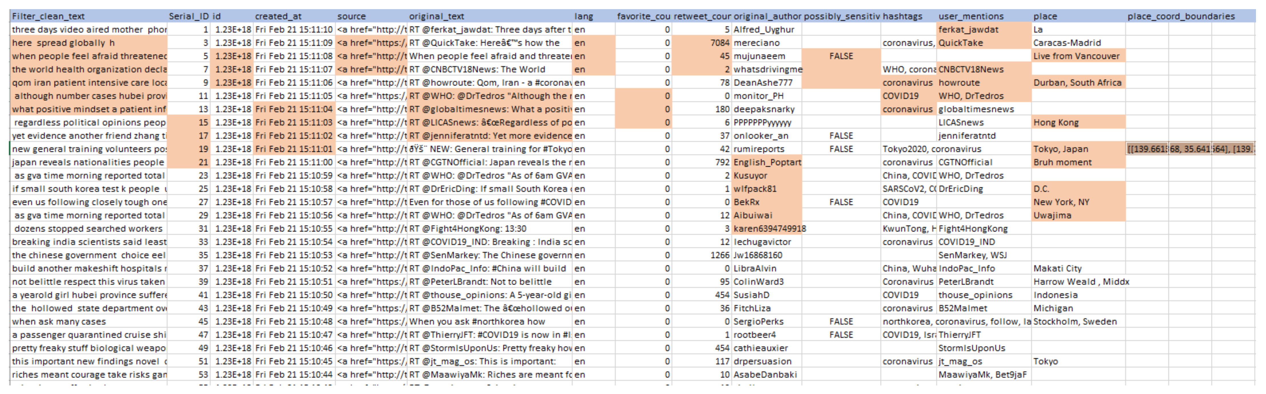
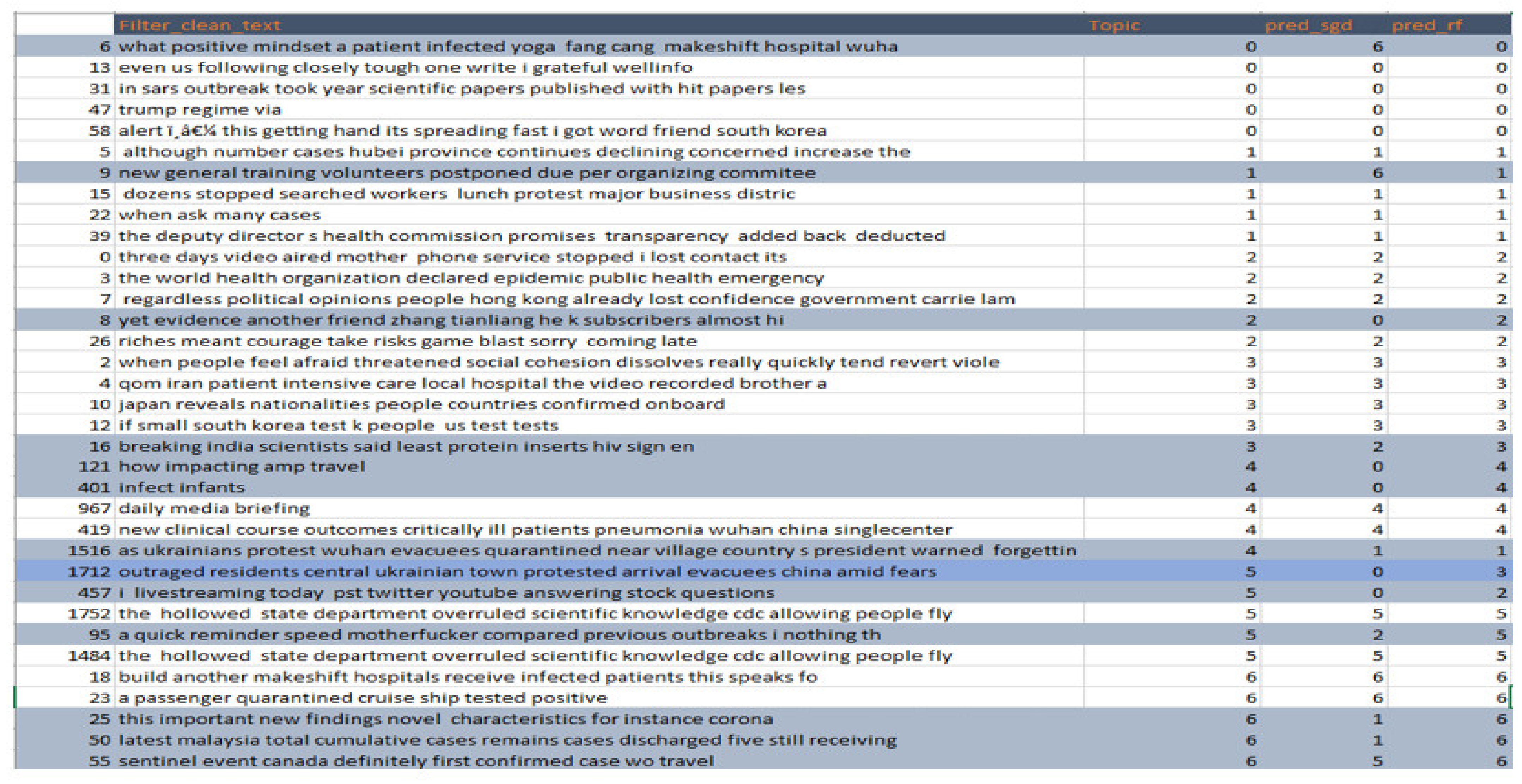
In our system, we scraped Twitter SMN data where several data fields construct our model and visualize data in a user’s intended way. Keeping up information quality is a troublesome yet fundamental undertaking. To accomplish predictable and dependable information, the model should continually oversee information quality so they build authenticity and enable quicker which produce more proficient decisions. We applied semantic, syntactic, consistency, completeness, and uniqueness to maintaining data quality. After removing repetition and contradictory data, it decreases the original length of size and provides freshness, timeliness, and actuality. The measurement is the interaction that actualizes the metric to acquire the value on the dimension factor. In a similar example of our dataset which is Covid data, the dimension exactness, the accuracy factor, the distinction in data field metric can be assessed by an evaluator utilizing a data cleaning function. For dimensionality reduction and increasing model accuracy, our total dataset reducing 3590 rows to 1795 rows with seven topic labeling. We have applied the same methodology in the Disaster dataset for our model verification. The scraping classifier in Section 4.1 has a Covid data field dimension which is based on the Twitter user’s statement.
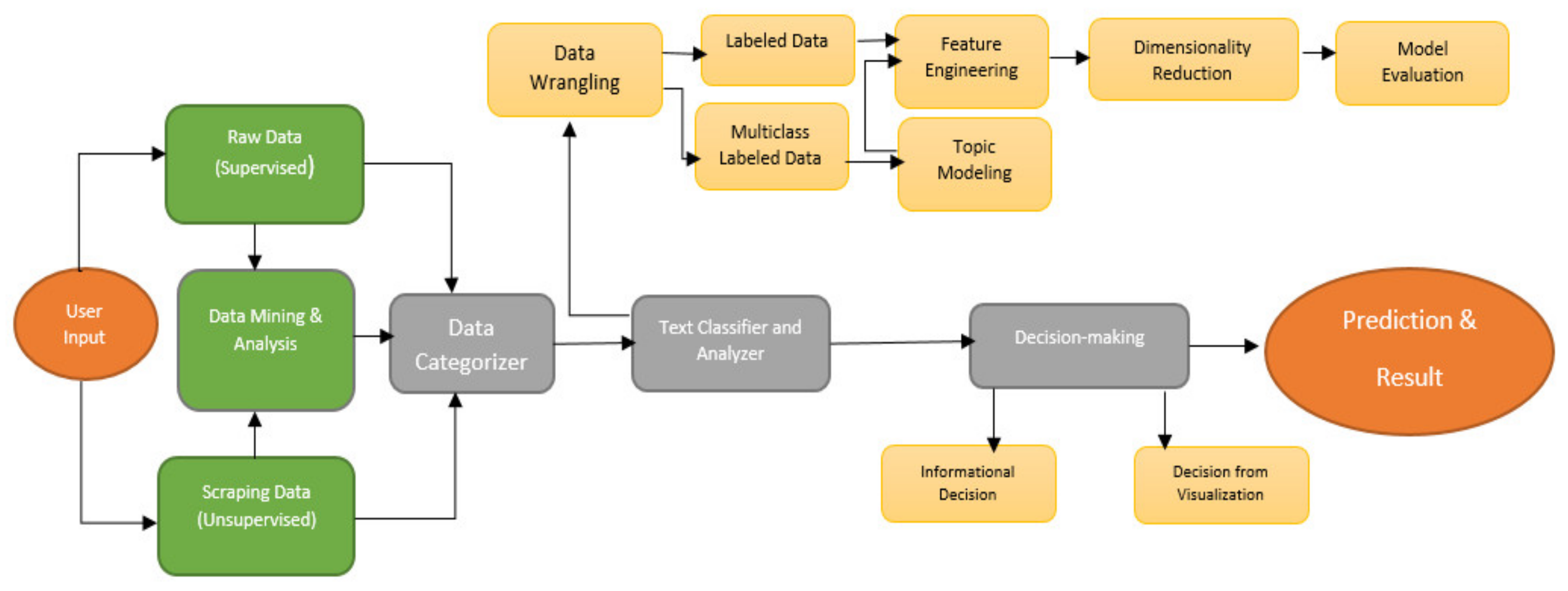
In supervised learning, there is a point at which we need to initially prepare the model with a previously existing, named dataset, much the same as showing a child how to differentiate between a seat and a table. We need to uncover disparities and similitudes. In contrast, unsupervised learning is tied to learning and predicting without a pre-named dataset. In the proposed RAIDSS model, there are two kinds of information input strategies: one is using labeled data, and the other is data mining. Users can input both types of information. Therefore, text classification is one of the most significant cycles for characterizing the user’s given info, choosing to order the data for unsupervised or supervised learning. If the data contain labeled information, then the text classifier and pre-processor execute data-wrangling extraction. After finishing a model assessment, the application takes the data for service and prediction. In contrast, if the information originates from Web scraping of various sources, numerous things (like data mining and analysis) need to be handled. The classifier’s objective should be to record clean information from the user and return the desired output. In discovering clean information segments, we need to conduct sentiment analysis to measure information execution and visualization. Topic modeling through Latent Dirichlet Allocation (LDA) and raw data conversion turn this unsupervised learning into a labeled dataset after information assembling, which provides structural performance and results.
We propose a real-time AI-based informational decision support system (RAIDSS) model for informational and DMSS systems in text classifications that include the following terminologies:
  • A filter cleaning text (FCT) methodology to scrape data cleaning and groupings;
  • A word generative probabilistic (WGP) method for highest word-frequency label selection;
  • A context-based chatbot application based on scraped datasets.
For the decision-making support system, the RAIDSS model visualizes data mining for the analysis of the topics (e.g., the current novel Covid and Disaster corpus); using Twitter data (namely tweets) for sentiment analysis; applying topic labeling for unsupervised and supervised learning (multi-class text classification); hyper-tuning data to provide robust application efficiency; visualizing data in various graphs, and comparing text classification methods. Finally, the chatbot provides an informational decision from among the supervised and unsupervised processes.
The remainder of this paper is organized as follows: Section 2 presents related work from the literature. Section 3 outlines the methodology of the working procedure in a system model. Data extraction and analysis determine if the corpus is supervised or unsupervised, which is discussed in Section 4. In Section 5, the text classifier assesses the model evaluation of both labeled and unlabeled data. Therefore, the chatbot takes the result of the assessment and gives an informational decision, as discussed in Section 6. Finally, evaluations of the prediction and development of the decision-making results are in Section 7.

2. Related Work

De Oliveira et al. [4] cited an architecture designed to monitor and perform anonymous real-time searches in tweets to generate information allowing sentiment analysis. These results show, data extraction from SMN gives information in real-time and they measure sentiment analysis at a low cost of implementation. It assists to make smart decisions in several environments. This work pretty much similar to our work but they only focus on sentiment analysis whereas the RAIDSS model provides not only scraping and sentiment analysis but also gives chatbot informational decision, known and unknown sentence prediction, Topic data groupings, valid or invalid group data accuracy, and finally DMSS.
Damaschk et al. [6] discussed methods of multiclass text classification on unstructured data which is one of our approaches to doing topic labeling for data grouping. Bevaola et al. [14] mentioned how to use Twitter data to send warnings and identify crucial needs and responses in disaster communication. Milusheva et al. [15] described how to transform an openly available dataset into resources for urban planning and development.
In text mining, Imran et al. [16] proposed artificial intelligence for disaster response (AIDR), a platform to perform automatic text classification of crisis-related communications. AIDR classifies messages that people post during disasters into a set of user-defined categories of information. Above all, the whole process must ingest, process, and produce only credible information, in real-time or with low latency [17]. In our RAIDSS model, data can be extracted from various sources, and pre-processing gives the exact user intention via the visualization and informational chatbot application.
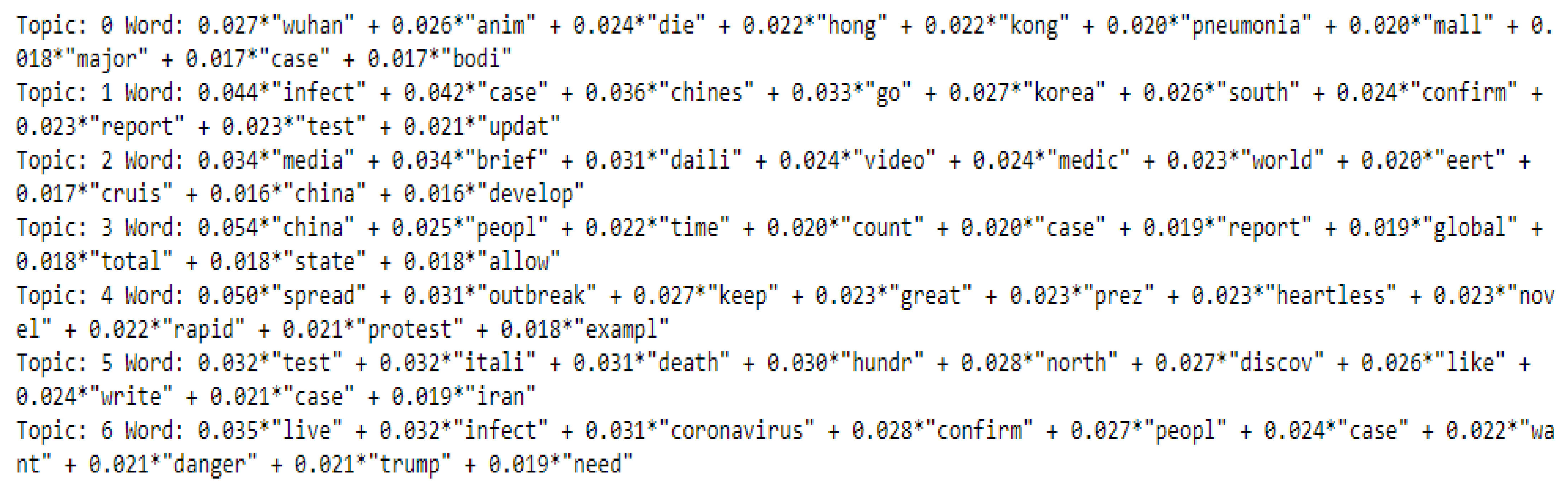
Topic models have numerous applications in natural language processing. Numerous articles have been published on topic modeling approaches to different subjects, for example, social networks, software engineering, and linguistic sciences [18]. Daud et al. [19] presented a review of topic models with delicate bunching capacities in text corpora, exploring essential ideas and existing models that sequenced different classifications with boundary estimations (i.e., Gibbs sampling) and performance evaluation measures. Likewise, Daud et al. introduced a few uses of topic models for displaying text corpora and discussed a few open issues with future directions. In our case, topic modeling uses multiclass text classification that labels a significant corpus as a category.
Dang et al. [
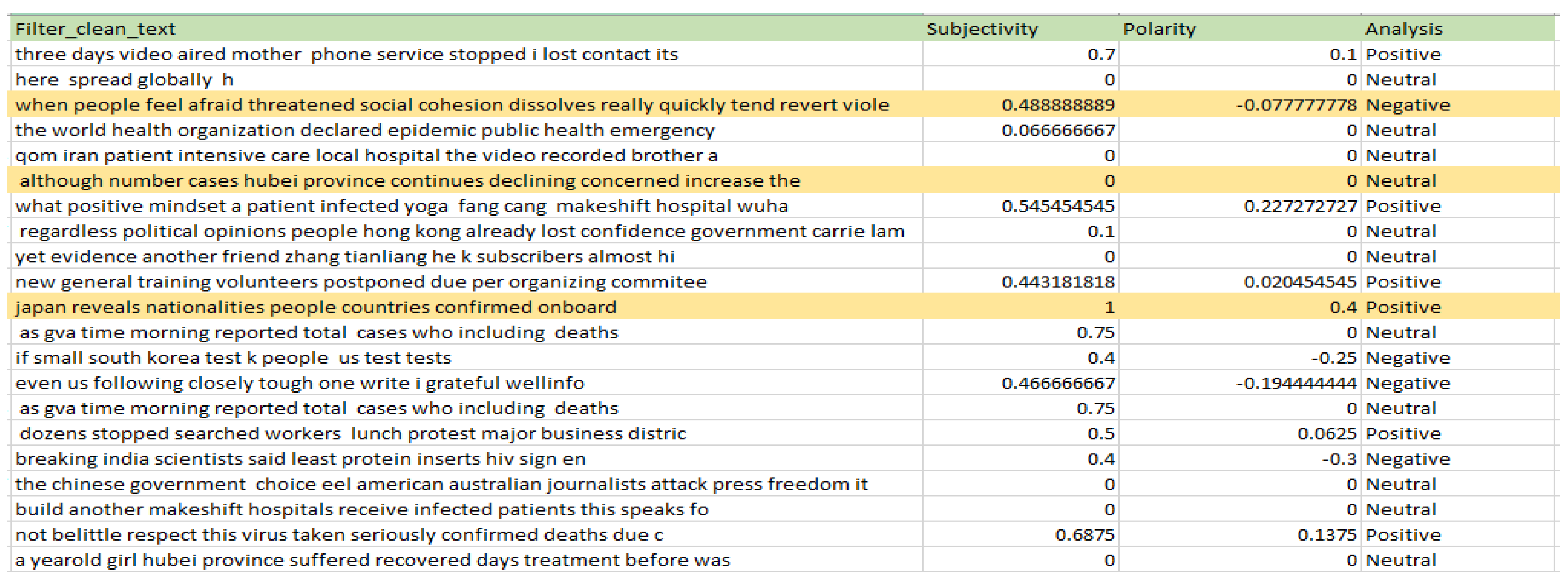
20] reviewed the latest studies that employed deep learning (DL) to solve sentiment analysis problems, such as sentiment polarity. Models used term frequency-inverse document frequency (TF-IDF) and word embedding procedures on a series of datasets. Sentiment analysis comprises language preparation, text examination, and computational phonetics to recognize abstract sentiments [21]. For the most part, new data entry samples have a similar category [
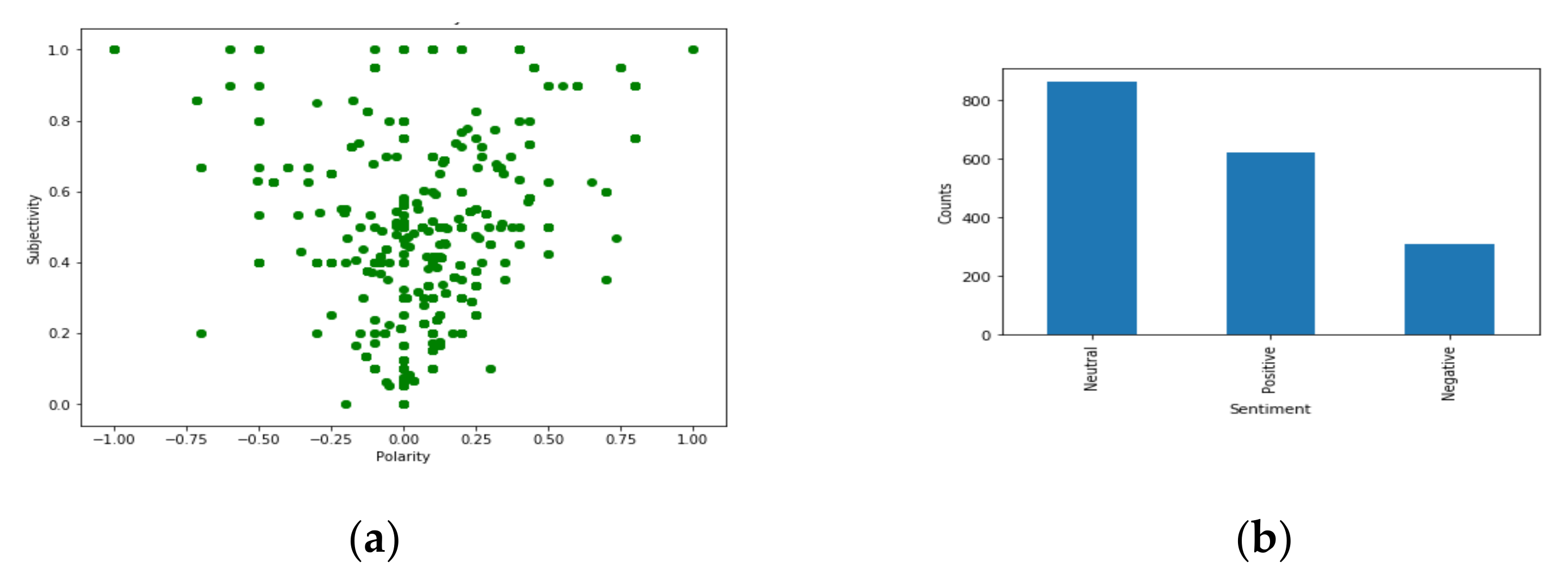
21]. Our model has an automated process for analyzing text data and sorting them into positive, negative, or neutral sentiments.
The semantic text-mining approach is significant for text classification. Škrlj et al. [22] presented a practical semantic content–mining approach, which changes semantic data identified from a given set of documents into many novel highlights used for learning. Their proposed semantics-aware recurrent neural architecture (SRNA) empowers the system to obtain semantic vectors and raw text documents at the same time. This examination shows that the proposed approach beats a methodology without semantic information, with the highest exactness gained (up to 10% higher) from short reports. Our methodology also shows useful semantic content from a model of an application where unstructured data make up useful content.
Most text classification and document categorization frameworks can be deconstructed into four stages: feature extraction, dimension reduction, classifier choice, and assessment. Kowsari et al. [23] talked about their survey and the structure and specialized usage of text classification frameworks. The initial input comprised a raw text dataset. Furthermore, Aggarwal et al. [24] mentioned text informational indexes contained groupings of text from records that alluded to a data point (i.e., a document, or a portion of text) with several sentences to such an extent that each sentence incorporated word and letters that include a class value from a set of diverse discrete word lists. The RAIDSS model proposed by us also takes this action in a particular manner to improve the outcome from information extraction.

3. Methodology

The RAIDSS classifier model is seen in Figure 1, where the user gives a specific keyword or topic to extract information from the Web or to specifically label the dataset to get results. After Web scraping or mining, the data need to be categorized for the classifier. The categorization process identifies which information is the user’s given and mining data. A text classifier formats these data for further analysis such as data preparation, model evaluation, builds an application and evaluates performance prediction and the results.
The objective of a text classifier is to send information to either supervised or unsupervised learning, where a given sample of data gets the desired output. It shows the relationships between input and output as visual information. After mining information that contains raw data, classifiers receive information as a named given dataset or as mined data. Therefore, the RAIDSS model does the assessment and provides the prediction or output. The most significant undertakings inside unsupervised learning are clustering, portrayal learning, and density estimation [25]. However, the dataset is prepared by topic modeling with multiclass text classifications, where the data-wrangling classifier first applies labeling and then goes into model evaluation. If the user input contains a labeling corpus, then the classifier sends it for supervised processing. Models have earlier information on what the output determines our samples ought to be. Thus, it is learning conceivable text and needs to apply binary or multiclass text classifications. Classification’s goal is to infer the natural structure or hierarchical structures that present data points [19]. After model evaluation, users get their desired answers through several decision-making graph visualizations and informational output by the chatbot application.

4. Data Mining and Analysis

Data mining programs separate patterns and associations in the information, depending on what data clients ask for or give. This process is used by companies to turn raw data into useful information. The data mining process breaks down into several steps [26]. First, organizations collect data and load them into their data warehouses [26]. Next, they store and manage the data, either on in-house servers or in the cloud. Business analysts, management teams, and information technology professionals access the data and determine how they want to organize them [26]. Then, application software sorts the data based on the users’ desired results; and finally, the end-user presents the data in an easy-to-share format, such as a graph or table [26]. Our model does the same thing, but the process is different. In our system, the classifier extracts data based on the users’ keywords. Therefore, a decision-making classifier creates a clean dataset, where information is measured by subjectivity and polarity (positive, negative, or neutral). Finally, Filter Cleaning Text sets up clean data where the information is organized.

4.1. Scraping Classifier

In the RAIDSS model assessment shown in Figure 2, the scraping classifier shows Twitter data extraction corpus by the users. Twitter’s API allows complex queries, like pulling every tweet about a specific keyword, or a user-mentioned keyword, within the last 20 min, the last few months or years, or by pulling a particular user’s non-retweeted tweets [27]. In our Web scraping application, tweets are analyzed for received information from the general user tweets, and classifiers collect the tweets that mention a specific topic. In the dataset, we extracted COVID-19 data from users, where the data fields include columns for ID, time created, the source, the original text, and hashtags, as well as fields labeled favorite_count, retweet_count, original_author, and user_mentions. We then run a sentiment analysis algorithm over them. We also target users who live in a specific location, known as spatial data. Another application could be to map the areas on the globe where topics have been mentioned the most. Twitter data can be a gateway to the general user’s insights and to how they receive information on a topic, which (combined with the openness and the generous rate-limiting of Twitter’s API) can produce powerful results [27].

4.2. FCT for Sentiment Analysis and Decision-Making

From the web scraping classifier, we extract text that is noisy data. So one specific column we need the most for our analysis is clean data. In RAIDSS classifiers, FCT is our developed function, which cleans data for handles, emoticons, emojis, and many regular expressions and stop words. Sentiment analysis is an automated process of identifying and extracting information that underlies a text [21]. It can be an opinion, a judgment, or a feeling about a particular topic or subject. The most common sentiment analysis type is called polarity detection, which involves classifying a statement as positive, negative, or neutral. It has two functions: one is to find the tweets, called subjectivity (how subjective or opinionated the text is—a score of 0 indicates a fact, and a score of +1 is very much an opinion); the other is to rate the tweets, called polarity (how positive or negative the text is—a score of −1 is the most negative, and a score of +1 is the most positive; 0 indicates a neutral statement). We used the TextBlob python library which helps to build our FCT method for analyzing the data. FCT gives a structured column, as seen in Figure 3, which is further used in model evaluation and results. Users can utilize sentiment analysis to assess any type of real-time informative decisions. In Figure 4, we tested the FCT approach in a disaster dataset and found that it produces relatable sentence-based decisions even though it was a huge corpus.
An excellent way to accomplish this task is by understanding the common words from plotting word clouds. A word cloud (also known as a text cloud or a tag cloud) is a type of visualization; the more a specific word appears in the text, the bigger and bolder it appears in the word cloud [28]. From this type of visualization, the RAIDSS model can determine a word from the corpus that occurs most often. Figure 5 and Figure 6 shows that the most prevalent words from Covid and Disaster corpus, which indicates that the model extracted the information impeccably.
In Table 1, we show the value counts from the data for how many positive, negative, and neutral items we have in our Covid classifier.
From the data, we visualize polarity and subjectivity as a scatter plot and a bar graph in Figure 7. It looks like most of the data are neutral, because many of the points are in the middle, at or near a value of 0.00. Total distributions of sentiment analyzers have value counts based on the analysis.

5. Text Classifier and Pre-Processor

Artificial intelligence (AI), machine learning (ML), and deep learning (DL) give data to machines for statistical pattern recognition [29]. Without a learning-model algorithm, a machine cannot analyze the performance and evaluate the process. In the literature, our text classification uses both ML and DL approaches and creates an application with an evaluation of its results. In our approach, we extract information from sources that generate unlabeled data. The extractor works most of the time to make unlabeled corpus data into labeled data without any pre-recorded information. It classifies raw data to determine the dataset’s intent. At the beginning of data extraction, algorithms learn from labeled data [30]. After understanding the intent, the algorithm finds a way to associate new data with patterns. For this reason, there are a few terminologies that are used to create clean data for the dataset. In the data wrangling process, NLP has several kinds of applications for processing, like word and sentence tokenization, removing stop words and capitalization, removing noise, correcting spelling, stemming and lemmatization, and many more.

5.1. Multiclass Labeled Data

Topic modeling efficiently analyzes large volumes of text by clustering documents into topics. With a large volume of unstructured data where the corpus has unlabeled meanings, we will not be able to apply our labeling approaches to create ML or DL models for these datasets. If we have unlabeled data, then we need to discover labels. In the case of text data, a cluster of documents is grouped by topic. LDA, an unsupervised generative probabilistic method for modeling a corpus, is the most commonly used topic modeling method [31]. It assumes that each document can be represented as a probabilistic distribution over latent topics, and assumes that topic distributions in all documents share a common Latent Dirichlet prior. Each latent topic in the LDA model is also represented as a probabilistic distribution of words, and the word distributions of the topics share this prior.
Given corpus D consisting of L documents, with document d having N d words ( d   1 , , L ), LDA models D according to the following generative process [31]:
  • Multinomial distribution φ t for topic t   t   1 , , T from a Dirichlet distribution with parameter β ,
  • Multinomial distribution θ d for document d   d   1 , , L from a Dirichlet distribution with parameter α , and
  • For a word, w n n 1 , , N d , in document d .
In the above generative process, words in documents are only observed variables, while others are latent variables ( φ and θ ) and hyper-parameters ( α and β ) [31]. To infer the latent variables and hyper-parameters, the probability of observed data D is computed and maximized as follows [31]:
p D | α , β = d = 1 L p ( θ d | α ) ( n = 1 N d Z d n p Z d n | θ d p ( w d n | Z d n , β ) ) d θ d
We divided the COVID-19 dataset into seven topic classes based on document similarity from the unstructured raw data. In Figure 8, Topic 5 has the most sentences from the whole corpus in the documents’ sentence distribution graph. In contrast, Topic 6 has the fewest from among the classes.

5.2. WGP Method for Topic Labeling in Covid Case

LDA expects documents to be from a mixture of topics [32,33]. Those topics, at that point, produce words dependent on the likeliest dissemination. Given a dataset of documents, LDA backtracks and attempts to make sense of the topics that would define those documents in the first place. This is a matrix factorization strategy [33]. In the vector space, any corpus (collection of documents) can be presented as a document–term matrix. The following matrix shows that corpus O reports D1, D2, D3...,Dn documents and a vocabulary size of F words W1, W2, W3,...,Wn. The estimation of the i , j cell gives the frequency count of word W j in document D i . LDA changes this document–term matrix into two lower-dimensional matrices: F1 and F2. F1 is a document–topics matrix, and F2 is a topic–terms matrix with dimensions (O, G) and (G, F) respectively, where O is the number of documents, G is the number of topics, and F is the vocabulary size, as seen in Table 2 [33].
LDA makes use of sampling techniques to improve topic word and document topic distributions which is the main aim of LDA. LDA iterates through each word, w, for each record, d, and attempts to replace the current topic–word task with a new task. Another topic, G, is appointed to word w with likelihood P, which is a result of two probabilities: p1 and p2. For every topic, probabilities p1 and p2 are calculated [33] as follows:
  • p1—p (t/d) = the proportion of words in documents d that are now appointed to point t.
  • p2—p (w/t) = the proportion of assignments to topic t over all the documents with word w.
Now, the current topic-word assignment is updated with the new topic and the model assumes that all the existing word-topic except the current word are correct. It is necessary the probability that topic t generated word w adjust the current word topics with new probability. The convergence point of LDA, after the number of iterations document topic and topic term distributions, is now impartially good.
Figure 9 shows that LDA can classify the text into topics, we chose randomly 7 categories for our dataset where the highest word frequency can choose the label name.
Now, we achieve a higher frequency of words by using LDA terminologies which is creating a word generative probabilistic method (WGP) in Table 3. It shows the highest frequency of words as a label name, which is more convenient for selecting data as a prediction.
The scraped dataset has 1735 sentences. We labeled this dataset with a topic number as well as a topic name (Place, Case, Media, China, Spread, Test, Live). In Figure 10, the filter_clean_text column shows which sentence belongs to which label.

5.3. Model Evaluations

At this stage, text and documents are now unstructured data sets. However, these unlabeled progressions must be converted into a structured feature space when using mathematical modeling as part of a classifier. First, the data need to exclude unnecessary characters and words. After processing, formal feature strategies are applied. The frequently used techniques for feature extraction are TF-IDF and Word2Vec [34].
For dimensionality reduction, we remove stop words and apply thresholds to the TF-IDF vectorizer, but it still leaves us with many unique words, many of which we probably do not need, and some are redundant. Let us also execute latent semantic analysis (LSA), a dimensionality reduction technique [35]. LSA uses singular value decomposition (SVD), and in particular, truncated SVD, to reduce the number of dimensions and selected the best.
For a model determination in ML, we selected various algorithms and contrasted them against the default parameters [36]. The enormous admonition here is that an algorithm may not perform well right out of the box, but it will with the correct hyper-parameters. This progression will give us a decent prime comprehension as to which sorts of algorithms (random forest, AdaBoost, stochastic gradient descent (SGD), KNN, Gaussian naive Bayes, decision trees) will naturally work better [36]. We chose six separate calculations to try out alongside the sklearn (Python library) dummy algorithm, which is merely an arbitrary possibility as a gauge. As for the measurements to assess the various algorithms, we are looking at accuracy, precision, recall, and F1 score.
At present, we have to explore different avenues regarding how our dataset functions in a deep learning approach. Our data source is a smaller dataset; that is the reason we are going to a recurrent neural network (RNN) utilizing LSTM engineering [37]. For large datasets, there are many approaches, like TextCNN and the bidirectional RNN (LSTM/GRU). LSTM was designed to overcome the issues of a primary RNN by permitting the system to store information in memory so it can access it sometime in the not-too-distant future. It is a particular sort of RNN that can learn long-haul designs. The way to use LSTM is with the cell express (a horizontal line going through the head of the outline) [38]. The cell state has been refreshed twice with barely any calculations that subsequently balance out the gradients. It likewise has a concealed express with demonstrations like short-term memory.

6. Informational Decision from Chatbot

For our model’s application, a chatbot provides a viable arrangement of the dataset. After concentrating the data by keyword, the user wants an informed decision based on the topic. There are two extensive variations of the chatbot: rule-based and self-learning. In a rule-based methodology, the bot responds to address dependence on certain principles that it is preparing. The principles characterized can be easy or complex. The bot can deal with fundamental questions, yet neglect complex ones. Self-learning bots are the ones that utilize some machine learning–based methodologies, and they are certainly more effective than rule-based bots [39]. These bots have categorization that is either retrieval-based or generative. For our RAIDSS model, a retrieval-based chatbot is congenial and depends on respect for the question and answer based on knowledge from the model [39]. We used a context-based chatbot that depends on respect for the user question and intense detection from the model.
The context-based chatbot is based on hyper-tuning dataset conditions, which structure the setting for an event, explanation, or thought and is (fundamentally, as far as it may be wholly comprehended) memory of all data about the users [40]. Memory that has earlier data about the users is gradually updated as the conversation advances. So (for gaining context), states and transitions are assumed to be a vital job here. Considering intent, to play out actions, users utilize the chatbot, which recognizes these activities by intent classification. According to the intent of the user, we place our chatbot in a particular state [41]. Transitions change the intent of the chatbot modes. There is an exchange mode starting with one state, then moving on to the next, which characterizes the discussions, and designs the chatbot. At the transition point, the chatbot requires a lot of data that belong to the same state. Due to the lack of data, it is harder to train the model. Neural networks work superbly at this stage, which is learning the context from the injected states.
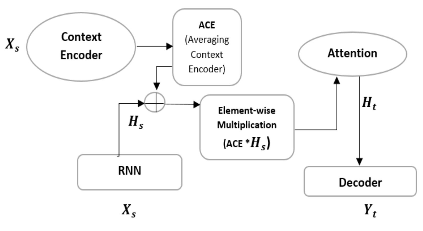
The RAIDSS functional chatbot model in Figure 11 describes context working on encoding input X s and aggregating output Y t through the averaging context encoder ( ACE ). Therefore, the training input layer, H s , from the RNN and ACE do element-wise multiplications right before feeding into the attention layer, H t . Finally, it decodes output layer Y t . The finite state machine uses this intent model input for text generation, which is a specific generative model. Each model will be generated based on the intended text, and will keep looping until the conversation stops.
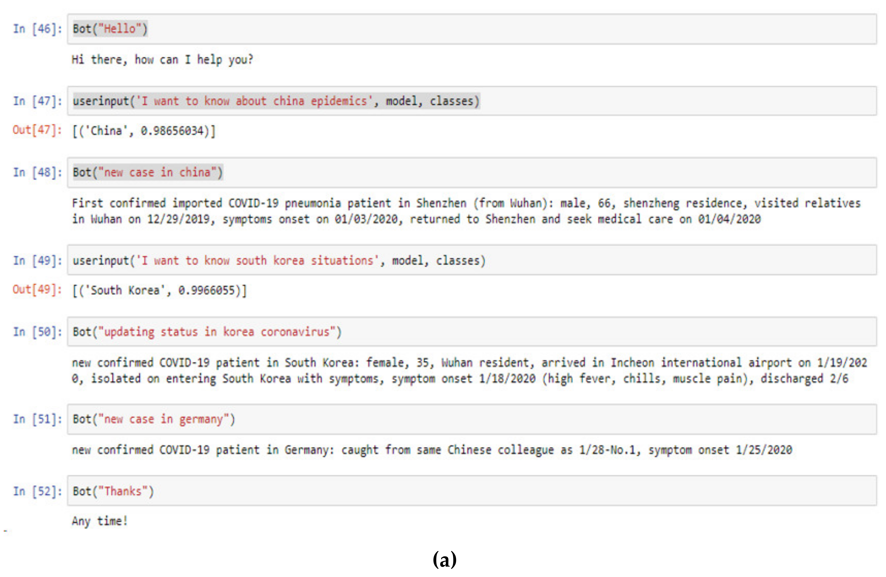
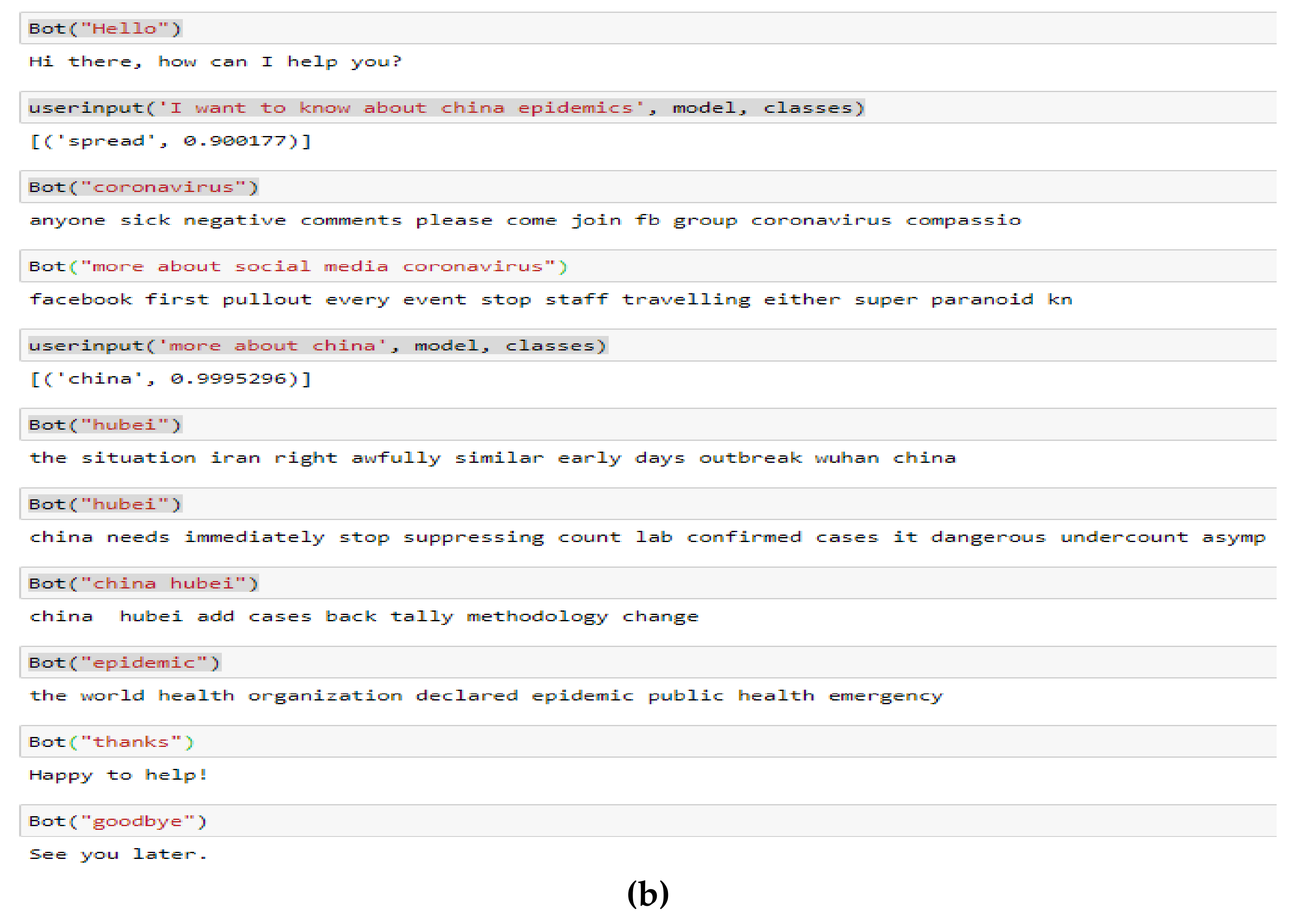
In Figure 12, we experiment with COVID-19 scraped data in part (a) COVID-19 labeled data, and part (b) our scraping data, where both give an informed decision. Labeled data show more meaningful information than scraped data because of the data length and the given information. In contrast to both datasets, the unlabeled chatbot decision in Figure 12b still gives an informative decision, though it has a noisy and small tweeter sentence.
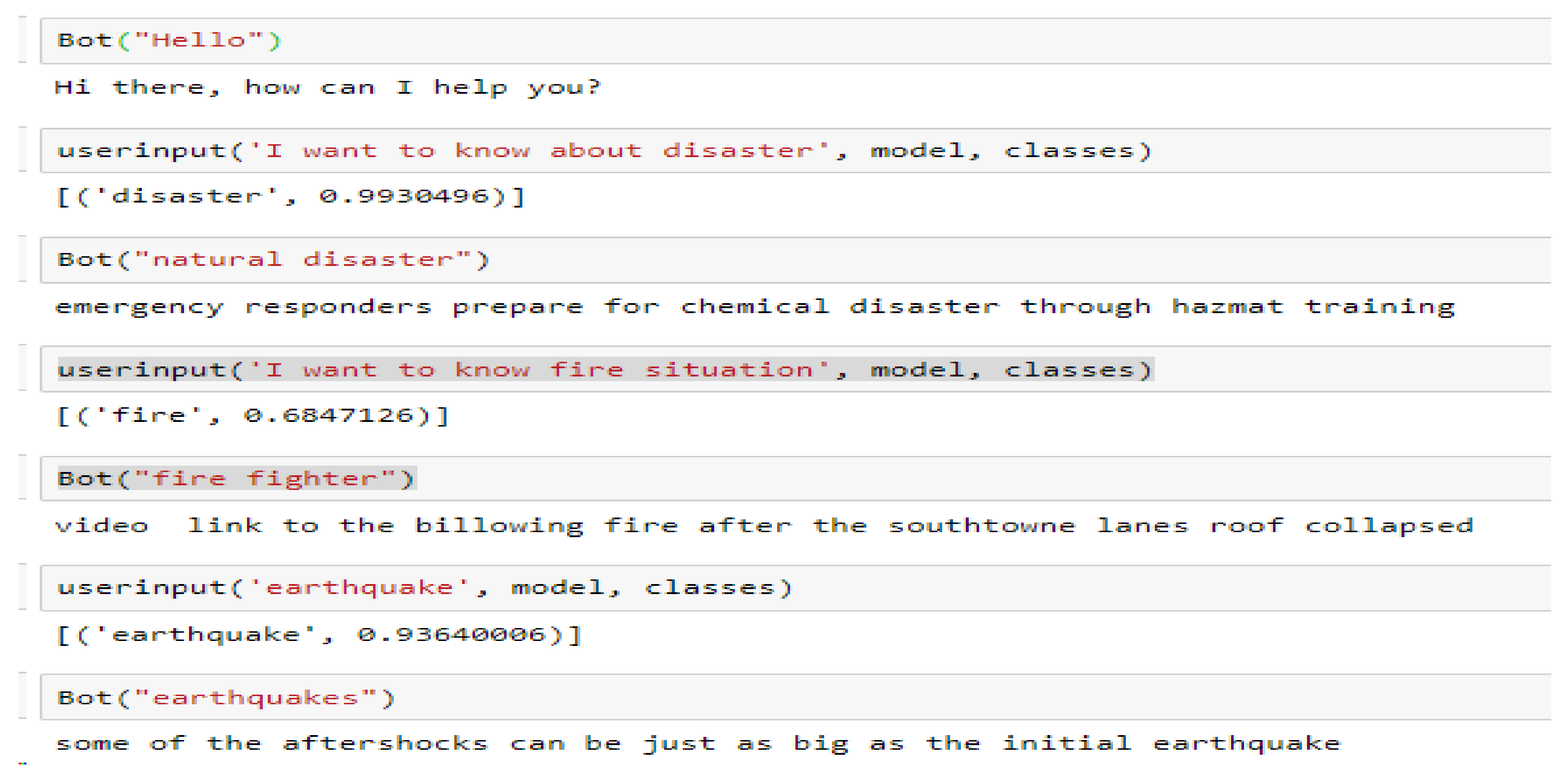
Our chatbot goal was to show data behaviors in unsupervised learning. For verification of our model, we offer a disaster dataset chatbot in Figure 13 which is in a large corpus. From the figure we can see that there has a piece of much relatable information along with disaster contents.

7. Evaluations of Decision-Making Support System

7.1. Machine-Learning Results in DMSS

For the decision-making support system in ML, we explored datasets where topic classes are already labeled [42]. We selected the average of these measurements as they were calculated per class. A macro averages the most helpful equations, which use F1 scores for each topic, and returns normal scores. A genuine test is for the way our information performs on inconspicuous articles. Table 4 for the coronavirus dataset performance where Random Forest had the highest F1 score (0.81), followed by the decision tree (0.79), and SGD (0.66). We experimented with two classifiers: RF and SGD. Here, in the simulation, we selected SGD because the decision tree and RF had nearly similar exactness, yet we show less precise results.
Hyper-parameter tuning returns the best outcome from the algorithms and our context-based chatbot application. It merely utilizes the default boundaries in our underlying evaluation, so they are not returned as well as can be expected. Using hyper-parameter tuning, the model needs to look through a good representation of the qualities to see which one works best [43]. For this situation, the Python library’s sklearn grid search with k-fold cross-validation is utilized. In k-fold cross-validation, the data are part of the k folds (five topics in the data we already separated). One out of the five parts from the data is used for testing, and the other four are used for preparation. Now, it happens k times, and each time an alternate overlay is used as the test set. The outcomes are from the median value. A matrix search experiences every single imaginable mix for all combinations for each hyper-parameter, and we return the best one, depending on the score.
For multiclass classification performance, AUC and ROC show better visualization of the datasets. This is one of the essential assessment measurements for checking any classification model’s presentation. An AUC close to 1 implies it has a decent proportion of detachability. A low model has an AUC close to zero, which implies it has the most exceedingly terrible detachability proportion, which implies responding to the outcome. Also, when AUC is 0.5, the model has no class detachment limit at all.
From our model, we now have the best parameters. Figure 14 has the ROC bend for (a) SGD and (b) RF, with micro and macro averages along with each class. We see in Figure 14a that SGD, class 0 (green), with the label Places is doing well among the classes, but class 5 (Test) and class 6 (Live) are battling the most. RF in Figure 14b has the best precision, and the F1 scores for our model in class 0 (Place) and class 3 (China) are closer to 1; class 5 (Test) is battling the most.
For model verifications, in the disaster corpus, there are five best topics model chooses which are 0, 1, 2, 3, and 6. Topics 4 and 5, on the other hand, do not provide any useful information regarding the contents. As a result, users may make an informed decision based on these topics among all the scraped content. In Figure 15, the Roc curve shows the RF method for micro and macro averages along with each class.
A confusion matrix is a precise method of visualizing the presentation of the prediction model. Every entry in a confusion matrix signifies the number of predictions made by the model and where it classified them effectively or incorrectly. Now, we have to look for where the point or class is mixing up the categories.
Figure 16a is the SGD diagram, which shows that the best F1 score expanded from 0.66 to 0.70 in the wake of tuning. It is a proper increment. In the SGD chart, Topic 5 (Test) and Topic 6 (Live) conflict the most with the other classes, and Topic 0 (Place) did great among the classes. In contrast, Figure 16b shows that the F1 score after tuning increased from 0.81 to 0.83, which is not awful. For RF, Topic 3 (China) and Topic 0 (Place) did well. However, Topic 4 (spread) conflicts a little with the different classes, particularly Place.
In machine learning prediction, the model assesses the selected and tuned information never before observed to see how it performs. The following are a few articles from each class we held out toward the start, alongside the prediction models prepared on the full dataset with the right class. We selected two algorithms (RF and SGD) that have great accuracy (RF) and center accuracy (SGD) for the predictions. From Figure 17, we can see that RF has a more exact prediction, instead of SGD. However, in most cases, RF and SGD anticipate a decent measure of information in the model.

7.2. Deep Learning Results in DMSS

In this task, we already classified our datasets into seven topics, and the model endeavors to anticipate which data belong to each class. In the deep learning experiment, we used LSTM modeling after applying multi-class text classification and data-wrangling classifiers to our datasets. In addition, we vectorized the COVID data, transforming all content into either a succession of whole numbers or into a vector. We limited the dataset to the top 50,000 words and set the maximum number of words in every objection to 250. Therefore, tokenization discovered just 2260 unique tokens. Machine learning works well with numbers. Subsequently, we created a method called text_to_sequences, which transforms all text into a sequence of integers, then takes each word from the documents and replaces each with its corresponding integer value from the dictionary tokenizer. If the word is not in the dictionary, it will insert a value of 1. For example, if we give the text “Paper writer has a pen on his table,” we will get the sequence: {2, 3, 4, 5, 6, 7, 1, 1}. The last two {1, 1} are for the term “his table,” which is not in the dictionary. We truncate and pad the information, grouping it, with the goal being to make them all a similar length. Table 5 shows a tokenization, labeling, training and testing data labeling chart for LSTM. A tensor can be started from the input information or the aftereffect of a computation. Here our identical data or shape of data is 1795 and the maximum number of words in every objection to 250 which makes the shape of data tensor (1795, 250) from Table 5. Therefore, we divide our dataset into seven topics which is the shape of the label tensor (1795, 7). In addition, we separate training data into identical data (1615, 250) and labeling (1615, 7). For the testing data split, the model chose (180, 250) and (180, 7). We give our model assessment via information split. In the short corpus, LSTM provides 99% accuracy. On the other hand, we conducted a test on a bigger corpus of Disaster datasets, and the accuracy was astonishingly high at 98%.
The model starts with an embedding layer that transforms the information’s whole-number lists into word vectors. Word embedding is an approach that expresses a word as a vector. It permits estimation of the vector’s component to prepare it. After preparing them, words with comparative implications frequently have similar vectors. Next, SpatialDropout1D performs a variation dropout in NLP models. The following layer is LSTM with 100 memory units, and the output layer must make seven types of output, one for every class. The activation function is softmax for multi-class classification because it is a multi-class grouping issue where categorical cross-entropy uses a loss function. In Figure 18, after 10 epochs, we obtained good accuracy from the training and testing datasets. We plotted in Figure 19 the history for accuracy and loss function to see if there was overfitting or not.
Next, we have to check how exact our data prediction is alongside known datasets and the new data. We predicted every sentence with seven topic labels. In both cases, it gave accurate predictions from among the labels, which are listed in Table 6.
In addition, we presented the same unknown sentence from disaster and Covid corpus prediction in Table 7, together with their labels and topic names. From the corpus, it has extracted relevant labels and names.

7.3. Decision-Making Support System from Text “Visulaization”

The decision support system involves several issues, such as foundation, functionality, interface, implementation, impact, and evaluation systems. We demonstrated our model which makes informed decisions using disaster and Covid datasets. The RAIDSS model creates DMSS foundations and functionality after processing text classifications in Table 8. By using the RAIDSS model, we get a diverse decision from an unlabeled dataset where we examined Twitter users’ tweets, reactions, and statements. A model aims to send information either supervised and unsupervised where a given corpus sample of data gets the desired outputs. For decision-making support system results, our dataset appertains to the Covid and Disaster case which is scraping from Twitter SMN where proposed terminology gives some specific decision. Mostly, FCT can give decisions from sentiment analysis and the WGP method gives corpus topic decision based on sentence categorization. Moreover, data accuracy from the ROC curve can say the advantageous decisions from the choosing best grouping label. Furthermore, Informational detailed decision from the Chatbot application and unknown sentence gives prediction based on training datasets.

8. Conclusions

We have developed an approach, from data mining to decision-making results, that measures through an informed decision how well data are created under unsupervised and supervised learning, and which data answer the users’ questions. The RAIDSS model scraped a small dataset also a large dataset for verifications and processed the data input into a decision result. One of the goals of our research paper was to see how a small dataset behaved in our model when compared to a larger dataset. For this reason, we used the larger corpus, which included disaster-related data, to test our hypothesis. We can see that the accuracy of both datasets is nearly identical, and the behavior of the data in the chatbot is unaffected. However, its procedures give the overall output from a noisy dataset. As we tested both machine learning and deep learning models, exactness and forecasts were acceptable. Additionally, our application was applied to extract specific information from keywords, which showed amazing predictions and results. The DMSS from the RAIDSS model aims to identify, analyze, and synthesize various supervised and unsupervised data. We tested the COVID case and Disaster corpus from Twitter scrapes of public statement, which give adequate visualization in sentiment analysis, the topic labeling decisions, the chatbot decisions, and finally, known and unknown sentence predictions. We’ll use this model in the future to work on speech and image classifications, as well as how to construct decision-making results.

Author Contributions

Supervision and investigation K.C.; A.I. are contributed equally in this paper for methodology and writing original draft preparation; writing-review and editing K.C., A.I., All authors have read and agreed to the published version of the manuscript.

Funding

This work was supported by Inha University Research Grant.

Institutional Review Board Statement

Not applicable.

Informed Consent Statement

Not applicable.

Conflicts of Interest

The authors declare no conflict of interest.

Abbreviations

The following abbreviations are used in the manuscript:
DTDocument Term
LDALatent Dirichlet Allocation
LSALatent Semantic Analysis
LSTMLong Short-term Memory
NLPNatural Language Processing
RFRandom Forest
RAIDSSReal-time AI-based Informational Decision Support System
SGDStochastic Gradient Decent
SMNSocial Media Network
SVDSingular Value Decomposition

References

  1. Thorstan, J. Text categorization with Support Vector Machines: Learning with many relevant features. In Machine Learning: ECML-98; Nédellec, C., Rouveirol, C., Eds.; Springer: Berlin/Heidelberg, Germany, 2005. [Google Scholar] [CrossRef] [Green Version]
  2. Franko, S.; Parlak, I.B. A comparative approach for multiclass text analysis. In Proceedings of the 2018 6th International Symposium on Digital Forensic and Security (ISDFS), Antalya, Turkey, 22–25 March 2018; pp. 1–6. [Google Scholar] [CrossRef]
  3. Devin, P. Social media Data Mining-How it Works and Who’s Using it. Available online: https://learn.g2.com/social-media-data-mining (accessed on 14 September 2020).
  4. De Oliveira Júnior, G.A.; de Oliveira Albuquerque, R.; Borges de Andrade, C.A.; de Sousa, R.T., Jr.; Sandoval Orozco, A.L.; García Villalba, L.J. Anonymous Real-Time Analytics Monitoring Solution for Decision Making Supported by Sentiment Analysis. Sensors 2020, 20, 4557. [Google Scholar] [CrossRef] [PubMed]
  5. Gajjala, A. Multi-Faceted Text Classification Using Supervised Machine Learning Models. Master’s Thesis, San José State University, San Jose, CA, USA, 2016; p. 482. [Google Scholar] [CrossRef]
  6. Damaschk, M.; Donicke, T.; Lux, F. Multiclass Text Classification on Unbalanced, Sparse and Noisy Data; Linköping University Electronic Press: Turku, Finland, 2019; pp. 58–65. [Google Scholar]
  7. Wang, J.; Xu, W.; Gong, Y. Real-time driving danger-level prediction. Eng. Appl. Artif. Intell. 2010, 23, 1247–1254. [Google Scholar] [CrossRef]
  8. Pinson, S.; Balbo, F. Using intelligent agents for Transportation Regulation Support System design. Transp. Res. Part C Emerg. Technol. 2010, 18, 140–156. [Google Scholar] [CrossRef]
  9. Tzima, F.A.; Mitkas, P.A. Strength-based learning classifier systems revisited: Effective rule evolution in supervised classification tasks. Eng. Appl. Artif. Intell. 2013, 26, 818–832. [Google Scholar] [CrossRef]
  10. Álvaro, H.; Emilio, C.; Alfredo, J. Unsupervised neural models for country and political risk analysis. Expert Syst. Appl. 2011, 38, 13641–13661. [Google Scholar] [CrossRef] [Green Version]
  11. Yu, B.; Lam, W.H.K.; Tam, M.L. Bus arrival time prediction at bus stop with multiple routes. Transp. Res. Part C Emerg. Technol. 2011, 19, 1157–1170. [Google Scholar] [CrossRef]
  12. Zarei, H.R.; Uromeihy, A.; Sharifzadeh, M. A new tunnel inflow classification (TIC) system through sedimentary rock masses. Tunn. Undergr. Space Technol. 2013, 34, 1–12. [Google Scholar] [CrossRef]
  13. Shadi, A.; Mehdi, G. Supervised and unsupervised learning DSS for incident management in intelligent tunnel: A case study in Tehran Niayesh tunnel. Tunn. Undergr. Space Technol. 2014, 42, 293–306. [Google Scholar] [CrossRef]
  14. Kusumasari, B.; Prabowo, N.P.A. Scraping social media data for disaster communication: How the pattern of Twitter users affects disasters in Asia and the Pacific. Nat Hazards 2020, 103, 3415–3435. [Google Scholar] [CrossRef]
  15. Milusheva, S.; Marty, R.; Bedoya, G.; Williams, S.; Resor, E.; Legovini, A. Applying machine learning and geolocation techniques to social media data (Twitter) to develop a resource for urban planning. PLoS ONE 2021, 16, e0244317. [Google Scholar] [CrossRef]
  16. Imran, M.; Castillo, C.; Lucas, J.; Meier, P.; Vieweg, S. AIDR: Artificial intelligence for disaster response. In Proceedings of the 23rd International Conference on World Wide Web (WWW ’14 Companion), Seoul, Korea, 7–11 April 2014; Association for Computing Machinery: New York, NY, USA, 2014; pp. 159–162. [Google Scholar] [CrossRef]
  17. Imran, M.; Lykourentzou, I.; Castillo, C. Engineering crowdsourced stream processing systems. arXiv 2013, arXiv:1310.5463. [Google Scholar]
  18. Jelodar, H.; Wang, Y.; Yuan, C. Latent Dirichlet allocation (LDA) and topic modeling: Models, applications, a survey. Multimed. Tools Appl. 2019, 78, 15169–15211. [Google Scholar] [CrossRef] [Green Version]
  19. Daud, A.; Li, J.; Zhou, L. Knowledge discovery through directed probabilistic topic models: A survey. Front. Comput. Sci. China 2010, 4, 280–301. [Google Scholar] [CrossRef]
  20. Dang, N.C.; Moreno-García, M.N.; De la Prieta, F. Sentiment Analysis Based on Deep Learning: A Comparative Study. Electronics 2020, 9, 483. [Google Scholar] [CrossRef] [Green Version]
  21. Pascual, F. Twitter Sentiment Analysis with Machine Learning. Available online: https://monkeylearn.com/blog/sentiment-analysis-of-twitter/ (accessed on 3 December 2020).
  22. Škrlj, B.; Kralj, J.; Lavrač, N.; Pollak, S. Towards Robust Text Classification with Semantics-Aware Recurrent Neural Architecture. Mach. Learn. Knowl. Extr. 2019, 1, 575–589. [Google Scholar] [CrossRef] [Green Version]
  23. Kowsari, K.; Meimandi, J.K.; Heidarysafa, M.; Mendu, S.; Barnes, L.; Brown, D. Text Classification Algorithms: A Survey. Information, Switzerland. Information 2019, 10, 150. [Google Scholar] [CrossRef] [Green Version]
  24. Aggarwal, C.C.; Zhai, C. A Survey of Text Classification Algorithms. In Mining Text Data; Aggarwal, C., Zhai, C., Eds.; Springer: Boston, MA, USA, 2012. [Google Scholar] [CrossRef] [Green Version]
  25. Jason, B. Supervised and Unsupervised Machine Learning Algorithms. Available online: https://machinelearningmastery.com/supervised-and-unsupervised-machine-learning-algorithms/ (accessed on 8 December 2020).
  26. Gupta, M.K.; Chandra, P. A comprehensive survey of data mining. Int. J. Inf. Tecnol. 2020, 12, 1243–1257. [Google Scholar] [CrossRef]
  27. Cuesta, Á.; Barrero, D.F.; R-Moreno, M.D. A Framework for Massive Twitter Data Extraction and Analysis. Malays. J. Comput. Sci. 2014, 27, 50–67. [Google Scholar]
  28. Heimerl, F.; Lohmann, S.; Lange, S.; Ertl, T. Word Cloud Explorer: Text Analytics Based on Word Clouds. In Proceedings of the 47th Hawaii International Conference on System Sciences, Waikoloa, HI, USA, 6–9 January 2014; pp. 1833–1842. [Google Scholar] [CrossRef]
  29. Wayne, T.; Li, H.; Alison, B. Artificial Intelligence, Machine Learning, Deep Learning and Beyond. Available online: https://www.sas.com/en_us/insights/articles/big-data/artificial-intelligence-machine-learning-deep-learning-and-beyond.html (accessed on 22 April 2021).
  30. Shang, W.; Dong, H.Z.; Wang, Y. A novel feature weight algorithm for text categorization. In Proceedings of the 2008 International Conference on Natural Language Processing and Knowledge Engineering, Beijing, China, 19–22 October 2008; pp. 1–7. [Google Scholar] [CrossRef]
  31. Blei, D.; Ng, A.; Jordan, M. Latent Dirichlet Allocation. J. Mach. Learn. Res. 2001, 3, 601–608. [Google Scholar]
  32. Arun, R.; Suresh, V.; Veni Madhavan, C.E.; Narasimha Murthy, M.N. On Finding the Natural Number of Topics with Latent Dirichlet Allocation: Some Observations. In Advances in Knowledge Discovery and Data Mining; Zaki, M.J., Yu, J.X., Ravindran, B., Eds.; Springer: Berlin/Heidelberg, Germany, 2010; Volume 6118. [Google Scholar] [CrossRef]
  33. Shivam, B. Beginners Guide to Topic Modeling in Python. Available online: https://www.analyticsvidhya.com/blog/2016/08/beginners-guide-to-topic-modeling-in-python/ (accessed on 6 December 2020).
  34. Liu, Q.; Wang, J.; Zhang, D.; Yang, Y.; Wang, N. Text Features Extraction based on TF-IDF Associating Semantic. In Proceedings of the 2018 IEEE 4th International Conference on Computer and Communications (ICCC), Chengdu, China, 7–10 December 2018; pp. 2338–2343. [Google Scholar] [CrossRef]
  35. Christopher, D.M.; Prabhakar, R.; Hinrich, S. Matrix decompositions & latent semantic indexing. In Introduction to Information Retrieval; Cambridge University Press: Cambridge, UK, 2012; pp. 403–417. [Google Scholar] [CrossRef]
  36. Bhumika; Sukhjit, S.; Nayyar, A. A Review Paper on Algorithms Used for Text Classifications. Available online: https://ijaiem.org/Volume2Issue3/IJAIEM-2013-03-13-025.pdf (accessed on 2 July 2021).
  37. Staudemeyer, R.C.; Morris, E.R. Understanding LSTM—A tutorial into Long Short-Term Memory Recurrent Neural Networks. arXiv 2019, arXiv:1909.09586. [Google Scholar]
  38. Jason, B. Sequence Classification with LSTM Recurrent Neural Networks in Python with Keras. Available online: https://machinelearningmastery.com/sequence-classification-lstm-recurrent-neural-networks-python-keras/ (accessed on 12 March 2021).
  39. Thosani, P.; Sinkar, M.; Vaghasiya, J.; Shankarmani, R. A Self Learning Chat-Bot from User Interactions and Preferences. In Proceedings of the 2020 4th International Conference on Intelligent Computing and Control Systems (ICICCS), Madurai, India, 13–15 May 2020; pp. 224–229. [Google Scholar] [CrossRef]
  40. Atiyah, A.; Jusoh, S.; Almajali, S. An Efficient Search for Context-Based Chatbots. In Proceedings of the 2018 8th International Conference on Computer Science and Information Technology (CSIT), Amman, Jordan, 11–12 July 2018; pp. 125–130. [Google Scholar] [CrossRef]
  41. Richard, C. Deep Learning Based Chatbot Models. arXiv 2019, arXiv:1908.08835v1. [Google Scholar]
  42. Kumari, S.; Saquib, Z.; Pawar, S. Machine Learning Approach for Text Classification in Cybercrime. In Proceedings of the 2018 Fourth International Conference on Computing Communication Control and Automation (ICCUBEA), Pune, India, 16–18 August 2018; pp. 1–6. [Google Scholar] [CrossRef]
  43. Derrick, M. How to Apply Hyper-Parameter Tuning to any AI Project. Available online: https://cnvrg.io/hyperparameter-tuning/ (accessed on 5 January 2021).
Figure 1. The RAIDSS text classifier model.
Applsci 11 06237 g001
Figure 2. Data extracted into specific columns based on user keywords.
Applsci 11 06237 g002
Figure 3. Covid clean dataset column where information for analysis is measured by subjectivity and polarity.
Applsci 11 06237 g003
Figure 4. Disaster clean dataset column where information for analysis is measured by subjectivity and polarity.
Applsci 11 06237 g004
Figure 5. Covid data visualization of words using a word cloud.
Applsci 11 06237 g005
Figure 6. Disaster data visualization of words using a word cloud.
Applsci 11 06237 g006
Figure 7. Sentiment analysis data in a scatter graph and a bar graph. (a) Polarity and subjectivity are shown in a scatter plot; (b) Sentiment analysis presents value counts in a bar graph.
Applsci 11 06237 g007
Figure 8. Documents’ sentence distribution graph.
Applsci 11 06237 g008
Figure 9. LDA word frequency per document sentence.
Applsci 11 06237 g009
Figure 10. Similarity check between text class and label.
Applsci 11 06237 g010
Figure 11. The neural network function-based context encoder with a Seq2Seq model for the chatbot application.
Applsci 11 06237 g011
Figure 12. Informational decision from the chatbot application: (a) contextual-based chatbot (supervised learning); (b) contextual-based chatbot (unsupervised learning).
Applsci 11 06237 g012aApplsci 11 06237 g012b
Figure 13. Informational decision from the disaster corpus chatbot application.
Applsci 11 06237 g013
Figure 14. Scraped coronavirus dataset where the ROC curves for SGD and RF have micro and macro averages along with each of the classes: (a) SGD ROC curve, and (b) RF ROC curve.
Applsci 11 06237 g014
Figure 15. Disaster scraped coronavirus dataset where the ROC curve chooses best classes.
Applsci 11 06237 g015
Figure 16. The scraped dataset’s confusion matrix to see where the classifier is mixing up categories: (a) the SGD confusion matrix, and (b) the RF confusion matrix.
Applsci 11 06237 g016
Figure 17. Prediction from a scraped dataset showing the performance of SGD and RF machine learning algorithms.
Applsci 11 06237 g017
Figure 18. Deep learning LSTM: (a) Training dataset accuracy is 0.99 and loss 0.04 and Testing dataset accuracy 0.96 and loss is 0.10 (b) Interpretations of F1, Precision and Recall performance is 0.90, 0.91 and 0.89.
Applsci 11 06237 g018
Figure 19. Loss and accuracy performance: (a) training and testing dataset loss vs. epochs, and (b) training and testing dataset accuracy vs. epochs.
Applsci 11 06237 g019
Table 1. An overall scraped data analyzer identifies neutral, positive, and negative data.
AnalysisCounts
Neutral865
Positive620
Negative310
Table 2. Matrix factorization figure that contains documents, topics, and vocabulary size.
W 1 W 2 W 3 W n G 1 G 2 G 3 G G 1 G 2 G 3 G
D 1 0213 D 1 1001 D 1 1001
D 2 1400 D 2 1100 D 2 1100
D 3 0231 D 3 1001 D 3 1001
D n 1130 D n 1010 D n 1010
Table 3. This is a table of labeled documents from the TF-IDF approach.
Classification LabelLabel NameWord Frequency Per Document
Topic 0Place0.027*“wuhan” 0.022*“hong” 0.022*“kong”
Topic 1Case0.044*“infect” + 0.042*“case”
Topic 2Media0.034*“media”
Topic 3China0.054*“China”
Topic 4Spread0.050*“spread”
Topic 5Test0.032*“test”
Topic 6Live0.035*“live”
Table 4. Algorithm performance on a coronavirus dataset processed with unsupervised learning.
Model NameAccuracyPrecisionRecallF1 Score
Random Forest0.840.850.790.81
Decision Tree0.830.790.790.79
Stochastic Gradient Descent0.670.840.610.66
K Nearest Neighbor0.640.710.580.61
Gaussian Naïve Bayes0.570.610.560.55
AdaBoost0.390.390.390.38
Dummy0.160.130.130.13
Table 5. Tokenization, labeling, and training in shaping the testing Covid data for the LSTM model.
Data Labeling ChartNumber
Shape of data tensor(1795, 250)
Shape of label tensor(1795, 7)
Train/test split(1615, 250) (1615, 7)
(180, 250) (180, 7)
Table 6. DL model prediction table for a known dataset vs. unknown text–data prediction.
Known Sentence Predictions
SentenceOriginal ClassClass NamePrediction
Chinese government chose American Australian journalists attack press freedom. 3 China 3
GVA time morning reported total cases including deaths.5Test5
Unknown Sentence Predictions
Government does not allow any reporter to enter an affected place. Unknown Place0
Table 7. DL model prediction table for both cases which gives unknown text–data prediction.
Natural Disaster Unknown Sentence PredictionsLabelTopic NameCoronavirus Unknown Sentence PredictionLabelTopic Name
“Korean government declare its pandemic situation in his country”0“News” “Korean government declare its pandemic situation in his country”4“Spread”
Table 8. Decision-making Support System (DMSS) table from the text.
Test TypeSource TypeDMSS Results
COVID “CASE”
DISASTER “CASE”
Coronavirus Twitter Scraped Data
Sentiment analysis (sentence polarity and subjectivity decision)
Decision-making support system (DMSS) analyzes the text and, based on sentences, measures sentiments. For example, “the world health organization declared epidemics in public health emergency” is a neutral sentence in polarity detection.
Topic labeling decision (the class or topic most of the sentence belongs to)
Most of the public review comments about the COVID “Test” class.
Most of the public review comments about the disaster “earthquake-1” class.
ROC curve decision (which topic/class is an accurate value or statement)
The “Place-0” class has the most accurate data among all the topics.
“earthquake-1” and “wildfir-6” class has the most accurate data among all the disaster topics.
Chatbot decision (informational detailed decision from data sources)
After the chatbot searches for “epidemics”, it returns an informational decision: “the world health organization declared epidemics in public health emergency”
After searching “natural disaster”, it returns an informational decision: “emergency responders prepare for chemical disaster through HAZMAT training”
Cloud visualization decision (keyword and data, how relatable to each other)
Most of the words in our sentence are related to Covid. For example, China, Outbreak, People, Place.
Most of the words in our sentence are related to disaster. For example, news, fire, earthquake, emergency, death, etc.
Deep learning model predicts known and unknown sentences, which gives decision results (any random sentence belonging to a class or topic).
From the unknown sentence prediction: “Korean government declares its pandemic situation in his country” it says our created class in Covid “Spread-4” and disaster corpus “news-0”.
Publisher’s Note: MDPI stays neutral with regard to jurisdictional claims in published maps and institutional affiliations.

