
Heuristic and Numerical Geometrical Methods for Estimating the Elevation and Slope at Points Using Level Curves. Application for Embankments


Abstract
:1. Introduction
2. Materials and Methods
| Algorithm 1 Solving IPS (denoted AIPS) |
| AIPS: Input: the points of the closest two level curves to Q Output: the shortest line segment [P1P2] that connects the given two level curves finished = false; While not finished do C = ϕ (empty set); Build the sets of line segments S1 and S2 (see Equation (2)); For each segment s1 from S1 do For each segment s2 from S2 do Calculate the shortest length segment P1P2 that connects s1 and s2 and passes through Q; If P1 ∈ s1 and P2 ∈ s2 then Add [P1P2] to C; End if; End for; End for; If C not is empty then finished = true; else k = k+1; End if; End while; |
2.1. Heuristic (Approximate) Method for SSTPC2L
| Algorithm 2 Solving the problem SSTPC2L |
| A1SSTPC2L: Input: Q and the points of the closest two level curves to Q Output: The slope at point Q Apply AIPS to find A11, A12, A21, A22; Calculate the point Pi by solving system of Equations (3) and (6) (i = 1, 2). Calculate the slope at point Q using Equation (1). |
2.2. The Exact (Mathematical) Method for SSTPC2L
- Translation with (−xI, −yI) (I is moved into origin O)
- Rotation with sin(−u) = −sin(u) and cos(−u) = cos(u), where:
- 3.
- Rotation with sin(v) and cos(v), where:
- 4.
- Translation with (−xQ, −yQ) (Q is moved into origin O)
- Translation with (−xQ, −yQ)
- Rotation with sin(u) and cos(u) (were calculated in (8))
- Rotation with sin(-v) = sin(v) and cos(-v) = cos(v) (calculated in (9))
- Translation with (xI, yI).
| Algorithm 3 Solving SSTPC2L |
| A2SSTPC2L: Input: Q and the points of the closest two level curves to Q Output: The slope at point Q Apply AIPS to find A11, A12, A21, A22; Transform the points A11, A12, A21, A22 and Q so that the bisector of the angle between the lines d1 and d2 is parallel to Oy axis and the point Q is in the origin O; Find the solution amin of the equation using bisection method on the interval (see Equations (19) and (20)); Calculate the coordinates of the points Pi (i = 1,2) using (13) and (14), where a = amin; Apply the inverse initial transformations in reverse order to the points P1 and P2; Calculate the slope at point Q using (1). |
3. Results
3.1. Elevation Estimation at a Point
3.2. The Slope between Two Points
3.3. Optimum Excavation/Filling
| Algorithm 4 Optimum Excavation/Filling (AOEF) |
| Input: the points Pi (i = 1, 2, ..., n) of the contour; for each point Pi do Find the closed discrete point P’i; end for; for i = 1 to n − 1 do Find the set of points Ci using Bresenham’s algorithm from point Pi to point Pi+1; end for; Using Bresenham’s algorithm from point Pn to point P1, find the set of points Cn; Find the points Qi (i = 1, 2, …, m) inside the contour given by C1 ∪ C1 ∪ … ∪ Cn; for each point Qi do Apply A2SSTPC2L to find the elevation zi of Qi; end for; |
| Algorithm 5 Height of Excavation/Filling Plane (AHEFP) |
| Input: vector of elevations z = (zi)i = 1, 2, …, m; Sort ascending the vector z; S = 0; for i = 2 to n do S = S + zi − z1; end for; S1 = 0; S2 = S; for i = 2 to n − 1 do S1 = S1 + (i − 1) ⋅ (zi − zi-1); S2 = S2 − (n − i + 1) ⋅ (zi − zi-1); if S2 ≤ S1 then opt = i; break; end if; end for; |
| Algorithm 6 Divide and conquer for optimum excavation/filling plane (ADCOEFP) |
| a = zopt-1; b = zopt; Sa,1 = S1 − (opt − 1) ⋅ (zopt − zopt-1); Sa,2 = S2 + (n – opt + 1) ⋅ (zopt − zopt-1); Sb,1 = S1; Sb,2 = S2; while b − a ≥ ε do c = (a+b)/2; Sc,1 = Sa,1 + (opt − 1) ⋅ (c − a); Sc,2 = Sa,2 − (n − opt + 1) ⋅ (c − a); if |Sc,2 − Sa,1| < |Sb,2 − Sc,1| then a = c; Sa,1 = Sc,1; else b = c; Sb,2 = Sc,2; end if; end while; S1 = Sa,1; S2 = Sa,2; |
3.4. Numerical Example
4. Discussion
- Avoid high erosion hazard sites, particularly where mass failure is a possibility.
- Utilize natural terrain features such as stable benches, ridgetops, and low gradient slopes to minimize the area of road disturbance.
- If necessary, include short road segments with steeper gradients to avoid problem areas or to utilize natural terrain features.
- Avoid midslope locations on long, steep, or unstable slopes.
- Locate roads on well-drained soils and rock formations which dip into slopes rather than areas characterized by seeps, highly plastic clays, concave slopes hummocky topography, cracked soil and rock strata dipping parallel to the slope.
- For logging road, utilize natural log landing areas (flatter, benched, well-drained land) to reduce soil disturbance associated with log landings and skid roads.
- Avoid undercutting unstable, moist toe slopes when locating roads in or near a valley bottom.
- Roll or vary road grades where possible to dissipate flow in road drainage ditches and culverts and to reduce surface erosion.
- Select drainage crossings to minimize channel disturbance during construction and to minimize approach cuts and fills.
- Locate roads far enough above streams to provide an adequate buffer, or provide structure or objects to intercept sediment moving down slope below the road.
- If an unstable area such as a headwall must be crossed, consider end hauling excavated material rather than using sidecast methods. Avoid deep fills and compact all fills to accepted engineering standards. Design for close culvert and cross drain spacing to effectively remove water from ditches and provide for adequate energy dissipators below culvert outlets. Horizontal drains or interceptor drains may be necessary to drain excess groundwater [13].
5. Conclusions
Author Contributions
Funding
Institutional Review Board Statement
Informed Consent Statement
Data Availability Statement
Conflicts of Interest
References
- Levin, A.H. Hillside Building: Design and Construction, US 2nd ed.; Builder’s Book Ink: Los Angeles, CA, USA, 1999. [Google Scholar]
- Tarbatt, J.; Tarbatt, C.S. The Urban Block—A Guide for Urban Designers, Architects and Town Planners; RIBA Publishing: London, UK, 2020; ISBN 9781859468746. [Google Scholar]
- Kicklighter, C.E.; Thomas, W.S. Architecture: Residential Drafting and Design; G-W Publisher: Tinley Park, IL, USA, 2018. [Google Scholar]
- Pyrgidis, C.N. Railway Transportation Systems: Design, Construction and Operation; CRC Press: Boca Raton, FL, USA, 2019; ISBN 9780367027971. [Google Scholar]
- Ellis, P. Guide to Road Design Part 1: Introduction to Road Design; Austroads Ltd.: Sydney, Australia, 2015. [Google Scholar]
- Fannin, R.J.; Lorbach, J. Guide to Forest Road Engineering in Mountainous Terrain; Rome (Italy) FAO: Rome, Italy, 2007. [Google Scholar]
- Deaconu, O.; Deaconu, A. Numerical methods to find the slope at a point on map using level curves. In IOP Conf. Series: Materials Science and Engineering, Proceedings of the Application in Road Designing, International Conference CIBv2019 Civil Engineering and Building Services, Brașov, Romania, 1–2 November 2019; IOP Publishing: Philadelphia, PA, USA, 2020; p. 789. [Google Scholar]
- Aruga, K.; Sessions, J.; Akay, A.E.; Ching, W. Forest Road Deisign and Construction in Mountain Terrain. In Proceedings of the Conference of IUFRO, Vancouver, BC, Canada, 13–16 June 2004. [Google Scholar]
- Sutton, R. An Introduction to Topography; Larsen and Keller Education: New York, NY, USA, 2017; ISBN 13 978-1635492774. [Google Scholar]
- Suresh, N.; Akhilesh, K.M.; Avijit, M.; Prasanta, S.; Praveen, E. Review of Alignment design consistency in Mountainous/Hilly Roads. In Proceedings of the 3rd Conference of Transportation Research Group of India, Kolkata, India, 17–20 December 2015. [Google Scholar]
- Jin, X.; Wei, L.; Yiming, S. New design method for horizontal alignment of complex mountain highways based on “trajectory–speed” collaborative decision. Adv. Mech. Eng. 2017, 9, 1–18. [Google Scholar]
- Siviero, L. Roads and Verticality Strategy and Design in Mountain Landscape. Ph.D. Thesis, Faculty of Engineering, University of Trento, Trento, Italy, 2012. [Google Scholar]
- Sheng, T.C. Watershed Management Field Manual, Food and Agriculture Organization of the United Nations; Rome (Italy) FAO: Rome, Italy, 1998. [Google Scholar]
- Quarteroni, A.; Sacco, R.; Saleri, F. Numerical Mathematics; Springer: Berlin/Heidelberg, Germany, 2007. [Google Scholar]
- Burden, R.L.; Faires, J.D. 2.1 The Bisection Algorithm, Numerical Analysis, 3rd ed.; PWS Publishers: Boston, MA, USA, 1985; ISBN 0-87150-857-5. [Google Scholar]
- Smith, A.R. Tint Fill. In SIGGRAPH ‘79: Proceedings of the 6th Annual Conference on Computer Graphics and Interactive Techniques; Association for Computing Machinery: New York, NY, USA, 1979; pp. 276–283. ISBN 978-0-89791-004-0. [Google Scholar]
- Bresenham, J.E. Algorithm for computer control of a digital plotter. IBM Syst. J. 1965, 4, 25–30. [Google Scholar] [CrossRef]
- Jadid, R.; Montoya, B.M.; Gabr, M.A. Strain-based Approach for Stability Analysis of Earthen Embankments. In Proceedings of the Dam Safety Conference, Online, Palm Springs, CA, USA, 21 September 2020–31 December 2020. [Google Scholar]
- Jiang, S.; Liu, X.; Huang, J. Non-intrusive reliability analysis of unsaturated embankment slopes accounting for spatial variabilities of soil hydraulic and shear strength parameters. Eng. Comput. 2020, 333, 1–14. [Google Scholar] [CrossRef]
- Rossi, N.; Bačić, M.; Kovačević, M.S.; Librić, L. Development of Fragility Curves for Piping and Slope Stability of River Levees. Water 2021, 13, 738. [Google Scholar] [CrossRef]


| Points | E (m) | N (m) |
|---|---|---|
| Q1 | 552,749.248 | 456,578.380 |
| Q2 | 552,754.270 | 456,571.835 |
| Q3 | 552,766.210 | 456,580.997 |
| Q4 | 552,760.244 | 456,588.772 |
| Q5 | 552,754.733 | 456,584.542 |
| Q6 | 552,753.385 | 456,581.554 |
| Points | E (m) | N (m) | Z(m) | Calculated Z(m) |
|---|---|---|---|---|
| Q1 | 552,749.2478 | 456,578.3797 | 707.8851 | |
| 552,749.7024 | 456,578.7371 | 707.6000 | ||
| 552,749.4725 | 456,578.9520 | 707.6000 | ||
| 552,748.8265 | 456,578.0230 | 708.0000 | ||
| 552,749.2769 | 456,577.9832 | 708.0000 | ||
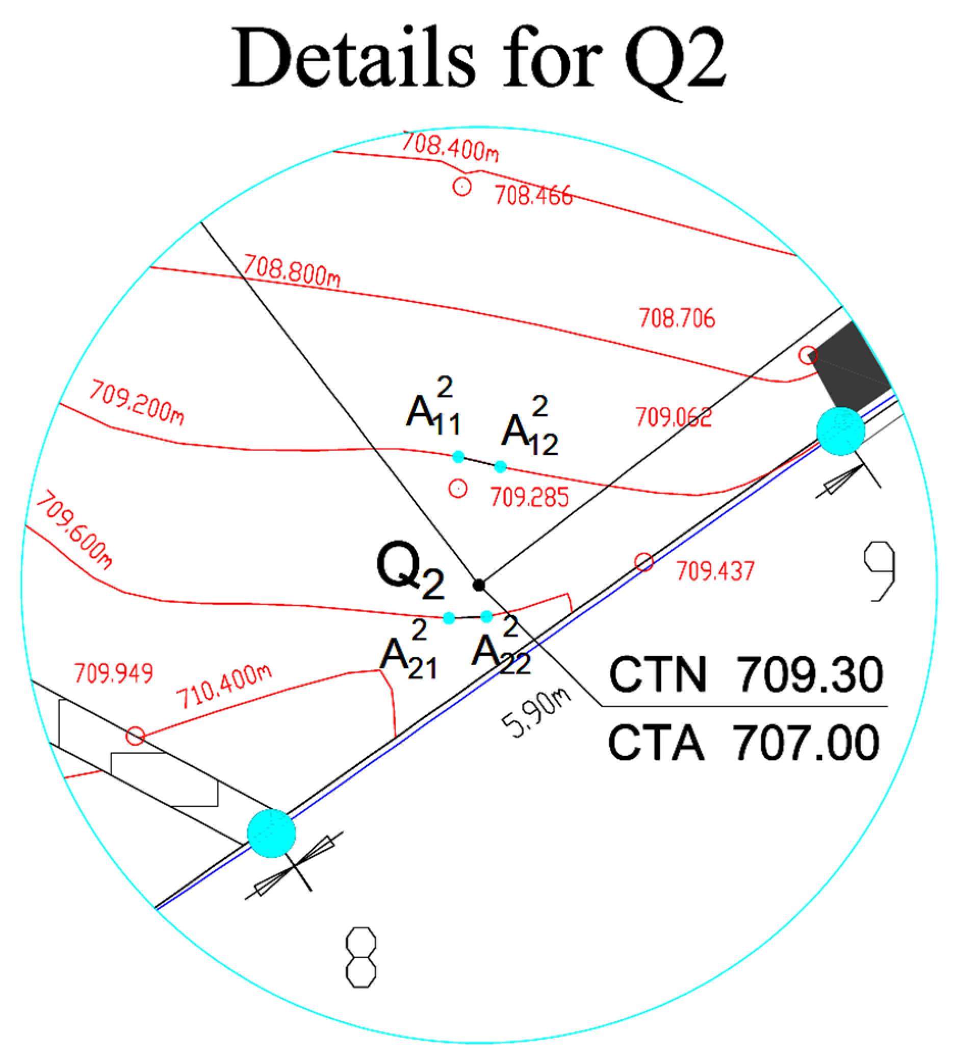
| Q2 | 552,754.2700 | 456.,571.8350 | 709.3279 | |
| 552,754.0980 | 456,572.9276 | 709.2000 | ||
| 552,754.4526 | 456,572.8445 | 709.2000 | ||
| 552,754.0176 | 456,571.5626 | 709.6000 | ||
| 552,754.3366 | 456,571.5767 | 709.6000 | ||
| Q3 | 552,766.2100 | 456,580.9970 | 704.2017 | |
| 552,768.2179 | 456,583.3340 | 704.0000 | ||
| 552,768.7357 | 456,582.6679 | 704.0000 | ||
| 552,760.8755 | 456,578.3463 | 704.4000 | ||
| 552,760.9848 | 456,577.8984 | 704.4000 | ||
| Q4 | 552,760.2440 | 456,588.7720 | 704.2330 | |
| 552,762.5489 | 456,590.7208 | 704.0000 | ||
| 552,762.9178 | 456,590.3418 | 704.0000 | ||
| 552,755.2345 | 456,585.1132 | 704.4000 | ||
| 552,754.9360 | 456,585.3872 | 704.4000 | ||
| Q5 | 552,754.7330 | 456,584.5420 | 704.7360 | |
| 552,755.2345 | 456,585.1132 | 704.4000 | ||
| 552,755.1438 | 456,584.4878 | 704.4000 | ||
| 552,752.7819 | 456,582.6377 | 704.8000 | ||
| 552,752.3362 | 456,582.9349 | 704.8000 | ||
| Q6 | 552,753.3850 | 456,581.5540 | 705.0855 | |
| 552,753.3671 | 456,581.7908 | 704.8000 | ||
| 552,753.7000 | 456,581.5900 | 704.8000 | ||
| 552,753.2125 | 456,581.6078 | 705.2000 | ||
| 552,753.5536 | 456,581.3981 | 705.2000 |
| Points | Estimated Z (m) | Measured Z (m) |
|---|---|---|
| Q1 | 707.8921 | 707.8990 |
| Q2 | 709.3279 | 709.3260 |
| Q3 | 704.2017 | 704.2140 |
| Q4 | 704.2330 | 704.2210 |
| Q5 | 704.7360 | 704.7500 |
| Q6 | 705.0855 | 705.0970 |
| Errors (First Method against Second Method) | |
|---|---|
| Lowest error | 0% |
| Average error | 0.61% |
| Highest error | 1.17% |
Publisher’s Note: MDPI stays neutral with regard to jurisdictional claims in published maps and institutional affiliations. |
© 2021 by the authors. Licensee MDPI, Basel, Switzerland. This article is an open access article distributed under the terms and conditions of the Creative Commons Attribution (CC BY) license (https://creativecommons.org/licenses/by/4.0/).
Share and Cite
Deaconu, A.M.; Deaconu, O. Heuristic and Numerical Geometrical Methods for Estimating the Elevation and Slope at Points Using Level Curves. Application for Embankments. Appl. Sci. 2021, 11, 6176. https://doi.org/10.3390/app11136176
Deaconu AM, Deaconu O. Heuristic and Numerical Geometrical Methods for Estimating the Elevation and Slope at Points Using Level Curves. Application for Embankments. Applied Sciences. 2021; 11(13):6176. https://doi.org/10.3390/app11136176
Chicago/Turabian StyleDeaconu, Adrian Marius, and Ovidiu Deaconu. 2021. "Heuristic and Numerical Geometrical Methods for Estimating the Elevation and Slope at Points Using Level Curves. Application for Embankments" Applied Sciences 11, no. 13: 6176. https://doi.org/10.3390/app11136176
APA StyleDeaconu, A. M., & Deaconu, O. (2021). Heuristic and Numerical Geometrical Methods for Estimating the Elevation and Slope at Points Using Level Curves. Application for Embankments. Applied Sciences, 11(13), 6176. https://doi.org/10.3390/app11136176