Ble Based Indoor Positioning System and Minimal Zone Searching Algorithm (MZS) Applied to Visitor Trajectories within a Museum

Featured Application

This paper introduces a new algorithm to retrieve the position of a user from BLE data, shaped as a zone. This algorithm has not sought to compete in terms of accuracy with already in place indoor positioning algorithm, but rather show a simple and new way to work with such data. This article also describes a typical indoor positioning experiment inside a museum that can be easily reproduced and that doesn’t need a lot of material.

Abstract

Museums are perfect experimentation grounds for indoor positioning technologies. Indeed, museum managers are always pleased to hold these kinds of events where it offers the opportunity to the public to be a part of such experimentation and allowing us at the same time to popularize our research with them. In this paper, we describe an experiment that held within the museum of natural history of La Rochelle with a class of high school volunteers. We will explain our systems that has been built to work in this specific case, and among other things formalize our algorithm for indoor localization that has not had an equivalent in the state of the art. The minimal zone searching algorithm (MZS) can compute in real time the position of a visitor, shaped as a zone with an average surface of 3 m${}^2$ when resources are limited and when the placement of nodes must respect the constraints imposed by the room’s layout. This method offered good results with data collected during the experimentation, such as a meaningful representation of the position of a visitor and most importantly a stable execution during the whole experience even when the subject was in tight spaces.

1. Introduction

The field of indoor positioning seeks the location of an individual, as we can have with GPS, but in a building [1]. As signals from satellites can’t go through walls in those places, a typical indoor positioning system is composed of a set of emitter sending a periodic signal (many types of signals are used such as radio frequency [2,3], ultrasound and infrared) [4,5,6] and a set of receivers. Based on the strength of the signal measured between an emitter and a receiver (called RSSI for Received Signal Strength Indication), the goal is to determine the position of the user within a room. Among all the signal used in such systems, the BLE (For Bluetooth Low Energy) became more and more popular since 2013, with the iBeacon technology designed specifically for indoor localization, with many applications such as [7].

In recent years, a certain number of indoor positioning studies are aiming to bring tracking technologies to museums [8,9,10]. Besides allowing museum managers to have a better overview of their places and thus having a better feedback on visits (which pieces of art are popular, and which ones are left), this also makes it possible to study behavior of visitors in such environments [11,12]. Moreover, museums are perfect experimentation grounds for indoor positioning technologies. Indeed, museum managers are always pleased to hold these kinds of events where it offers the opportunity to the public to be a part of such experimentation and allowing us at the same time to popularize our research with them. On top of that, visitors stay a long time within the same room and walk slowly, which allow us to better capture their path.

But museums also bring with them constrains that indoor localization researchers have to deal with. First, some studies apply machine learning algorithm for indoor localization systems as explain in [13], offering incredible accuracy values and great results overall. It’s very difficult to use such methods in museums, as it will take a lot of resources and time to collect data in order to train those models that will only work on one museum (As the architecture and room layout is not the same between museums). Second, we are limited in the number and placements of nodes for our indoor positioning systems. Indeed, our nodes should not disturb visitors during their tours (so we can’t place them in the middle of the way) and we have to work around artwork and room layout that were not always designed to accommodate an indoor positioning system.

In this paper, we will describe our indoor positioning experimentation and the system we used to get the position of a visitor, that can be used in real-time. Beside the data process architecture, we will propose a new algorithm which at our knowledge has not had an equivalent in the state of the art and that we named the minimal zone searching algorithm (MSZ). We will then show that this algorithm allows use to get the position of a visitor as a zone with an average surface of 3 m${}^2$ even when the placement of the nodes is not optimal.

2. Materials and Methods

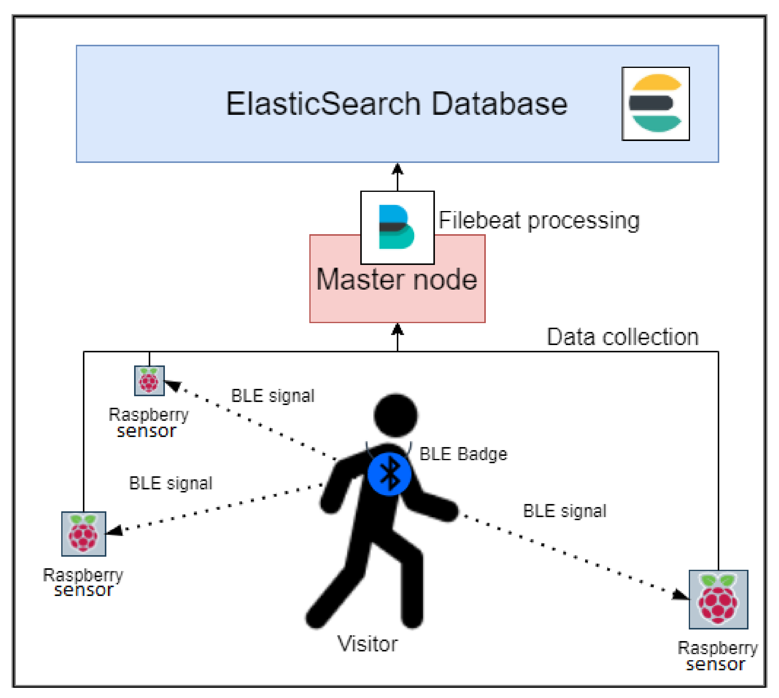
2.1. Our Indoor Positioning System

Our indoor positioning system is composed of a set of Raspberry Pi (Study like [14] used a similar system) playing the role of sensor and badges to wear around the neck sending a BLE signal. Most indoor localization approaches tend to use smartphone applications, but as we wanted to be as simple as possible, a basic necklace doesn’t require too much investment from visitor and is less intrusive. Also, it avoids technical problems such as storage, type of phone or its version etc.

In Figure 1 we can see a representation of our system of indoor positioning.

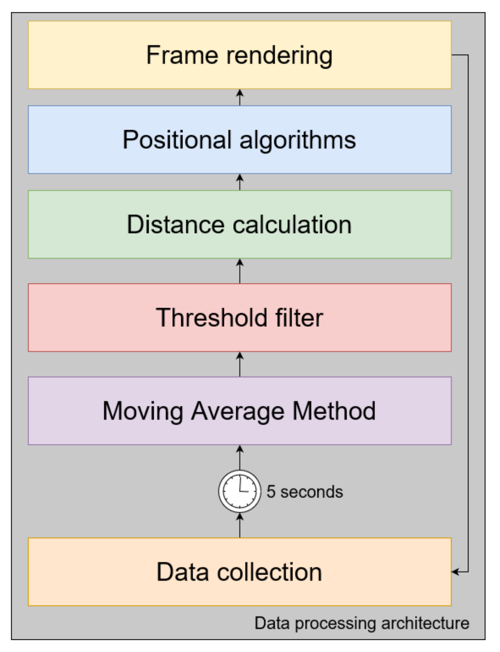
2.2. Data Processing

Figure 2 explain our data processing architecture in real time. The data collection step follows Figure 1 directly. The position of the user is monitored during n seconds, when n is the value of the time parameter, in this paper, we used a time window of 5 s. The transmission frequency of our BLE emitter is 1 Hz. We collect data during 5 s and then we apply the following steps of the data preprocessing. Using only BLE signal in an indoor positioning system expose us to use data subject to imprecision and outliers. We then need to collect a certain amount of data to overcome them.

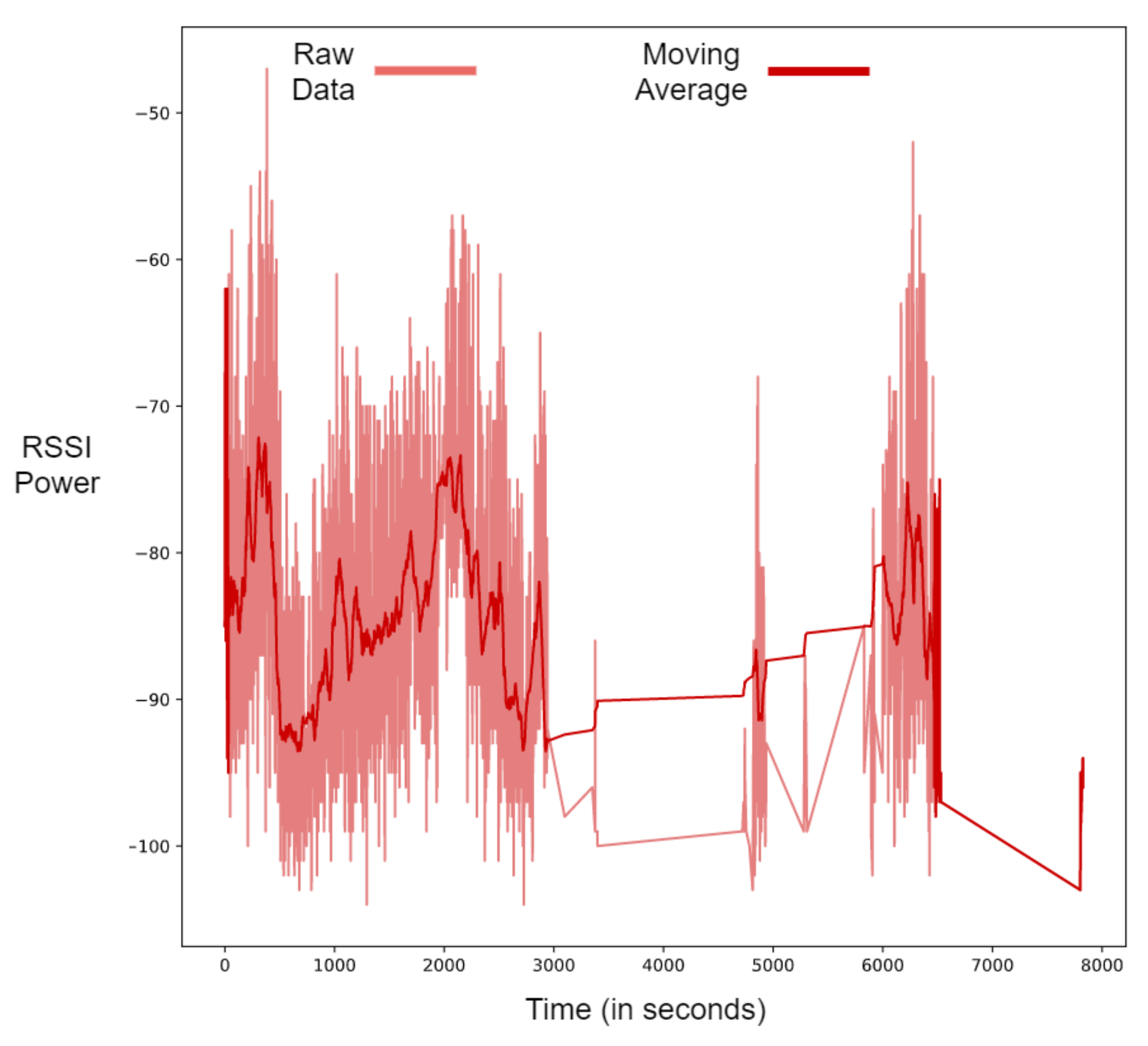
2.2.1. Moving Average Method

The moving average method is frequently used in indoor positioning systems [15,16,17] as it reduces the value of outliers and smooths the signal making it easier to process.

Figure 3 shows the impact of the moving average method on raw data collected by one sensor, smoothing the signal and making it easier to process by removing the drastic variation in our values.

2.2.2. Threshold Filter

The threshold filter step consists to compute the mean value of all RSSI data after the moving average output, and then decide if the sensor is relevant or not. Indeed, in our case the museum has several floors and sometime the BLE signal sent by the visitor’s badge passes through the ceiling. In this paper, we won’t take into account an RSSI value lower than −90 dB. Meaning that we consider that the visitor is not in the studied room if the value is less that the threshold value. The output of this step is a list of sensors and their associated average RSSI value during the last 5 s.

2.2.3. Distance Calculation

The RSSI distance measurement uses the logarithmic distance path-loss model, used in several studies using BLE signals such as [17,18]:

$$L_s=(-10n)lo{g}_{10}\left(RSS{I}_s\right)+L_0$$

where $L_s$ is the distance in meter based on the RSSI value of sensor s, n is the broadcasting power value (2 in our case) and $L_0$ is the measured RSSI power at 1 m. In our case, $L_0$ is equal on average to −62 dB, but it is mandatory to keep in mind that this value can drastically change depending on the environment (such as the size of the room studied) and thus this constant must be measured in all new environments.

2.2.4. Positional Algorithms

In this step we apply the positional algorithms requested. Three algorithms have been used during this experimentation.

(1) Triangulation:

The triangulation algorithm such as explain in [19] have been used as it was suitable to our problem. The only minor adjustment we made is that we take into account the zone between all intersection points as a potential position of the visitor. As we are working with data coming from a window of 5 s, a zone is more representative in this context.

(2) Trilateration:

The trilateration algorithm explained in [20] and often used in BLE based indoor positioning works such as [21,22,23] returned poor results in our case. It may come from the non-optimal placement of our sensors within the room (Such as the “grid” placement), the exclusive use of BLE signal and the 5 s window of data collection which is not suitable for accurate and precise localization in a single point (x, y) of the visitor. In the majority of cases, the trilateration did not return any position.

(3) Minimal zone searching algorithm (MZS):

We also used our proposed algorithm, the MZS algorithm, which will be described in the next section. Considering all sensors within the room, it iterates until getting the minimal zone, representing the movement of a visitor.

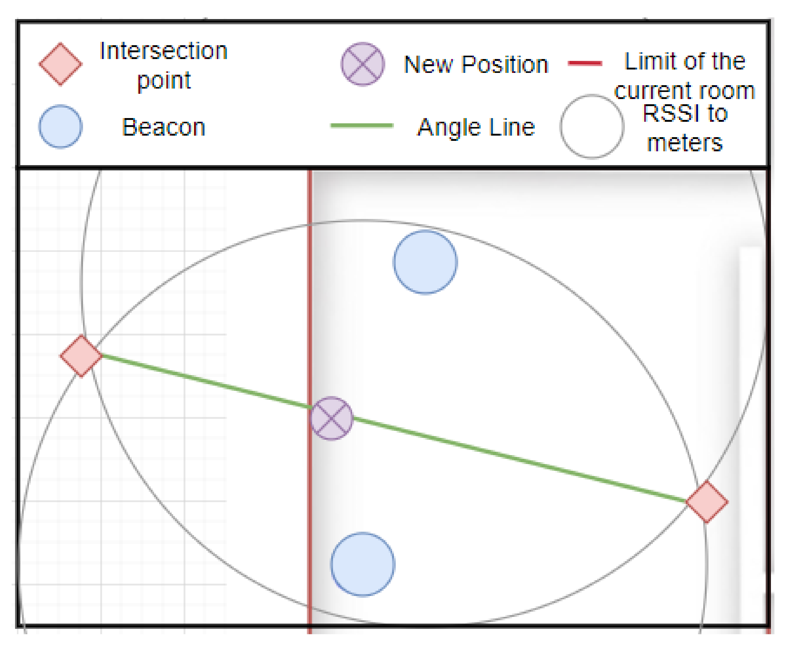
(4) Recalibration:

We used a common method for all positional algorithms. When a calculated point such that circle intersection with the triangulation or a ${\Gamma }_s$ point (The key part of the MZS that we will explain in the next section) is located outside the studied room, we put it down at the limit of this one as described in Figure 4.

The angle line in Figure 4 connects a reference point with the point outside the room in order to determine the angle of the intersection with the limit of the room. This reference point is the second intersection point in the triangulation algorithm, and the corresponding ${\Gamma }_s$ point for sensor s in the proposed algorithm. This simple method has offered significant results in our case.

2.2.5. Frame Rendering

The final step of the data processing architecture is the frame rendering. As our system seeks to render in real time a positioning suggestion, the system will display the current position of the visitor in the room each 5 s. The frame rendering is made in python using the library matplotlib.

3. Minimal Zone Searching (MZS), a New Positional Algorithm

The goal of the proposed algorithm is to find the smallest possible zone where the visitor is likely to be at a certain point in time. As we saw in the previous section, we are working with data coming from sensors based on a time window of 5 s.

Most approaches in indoor positioning systems, such that trilateration or triangulation only takes three to four sensors who recorded the maximum value of RSSI. With this approach we are taking into account all sensors in the room. The algorithm considers the set S of sensors as input, each sensor $s\in S$ is given by its coordinates ($x_s$, $y_s$) and its RSSI value $L_s$, and computes a minimal zone as the representation of possible positions of the individual. The algorithm iterates until a the optimal zone is reached. At each iteration i, a new zone $zon{e}_i$ is computed from the centroid of the zone issued from the previous iteration and the RSSI values of each sensor s. The treatment is initialized with the first zone $zon{e}_0$ defined as the convex hull of sensors within the room (Equation (1)):

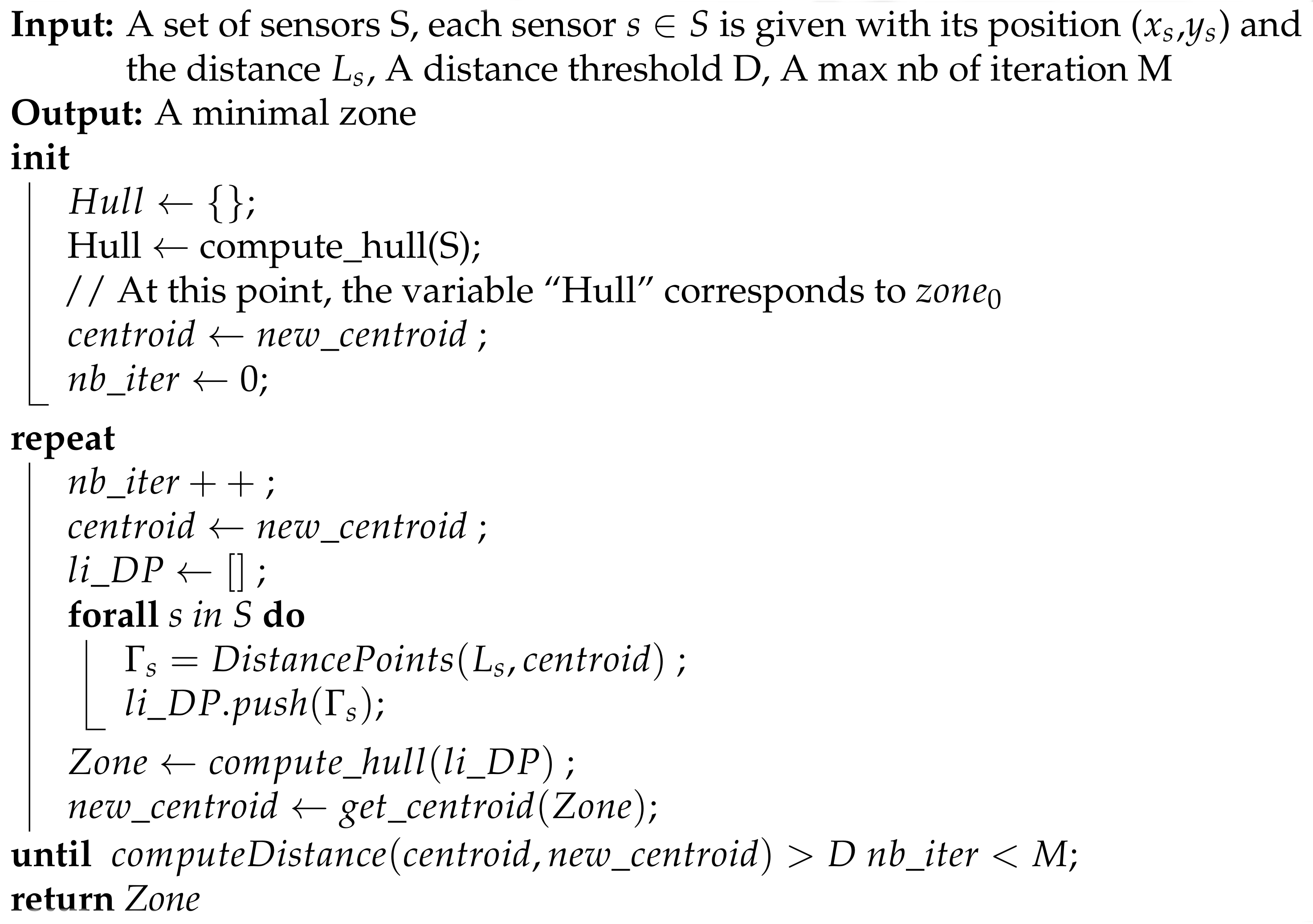
The MZS algorithm (Algorithm 1) starts by computing the convex hull of sensors within the room, as explained in Equation (1), $zon{e}_0$ represents the initialization step.

$$zon{e}_0=Hull\left(x_s,y_s:sensors\right)$$

(1)

The zone is then refined as the convex hull of a set of distance points, each distance points ${\Gamma }_s$ is computed from a sensor s and the value of $L_s$ according to the centroïd c of the previous convex hull: (Equations (2) and (3)).

$${\Gamma }_s=\left[\begin{array}{c}{x}_c\\ y_c\end{array}\right]+L_s\left[\begin{array}{c}cos\left({\alpha }_s\right)\\ sin\left({\alpha }_s\right)\end{array}\right]$$

(2)

where we consider a set of sensors noted b described by their coordinate $b:(x_s,y_s)$, and $L_s$ is a distance in meter computed based on the RSSI value returned by a sensor s at a time t. The centroid $C_0(x_c,y_c)$, ${\alpha }_s$ the angle in radiant between the centroid C and sensor s. The next execution (n=1), consider the convex hull of all ${\Gamma }_s$ point and the new centroid $C_1$. The iteration of the zone calculation is based on the following equation:

$$zon{e}_i=Hull\left(\{DistancePoints(L_s,C_{zon{e}_{i-1}}):sensors\}\right)$$

(3)

where $C_{zon{e}_{i-1}}$ is the centroid of the $zon{e}_{i-1}$ and DistancePoints() is a direct reference to Equation (2).

Algorithm 1: Minimal Zone Searching.

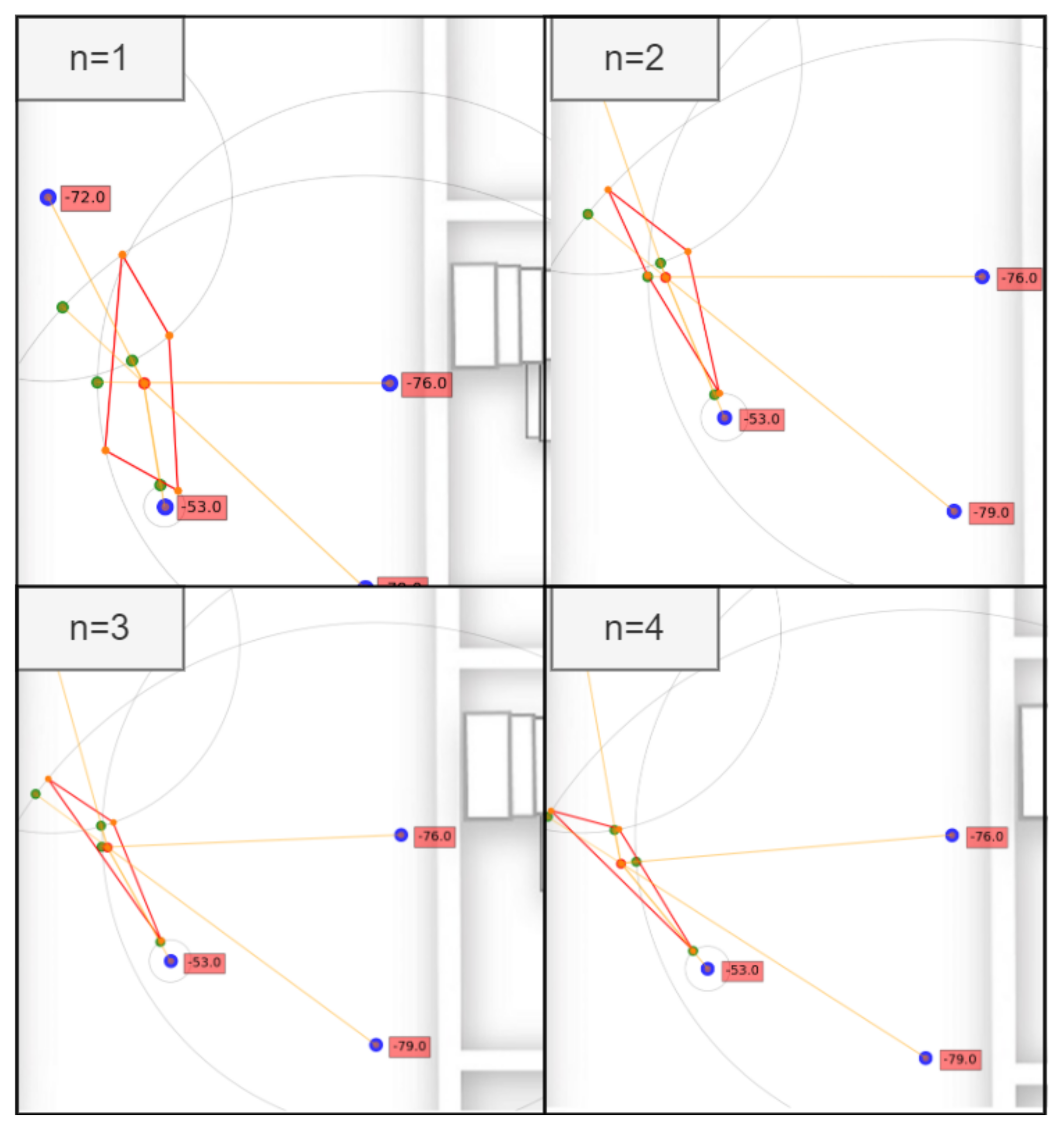
The algorithm will stop when the size and position of $zon{e}_{i-1}$ and $zon{e}_i$ are comparable and where only minor changes occur, or if we reach the maximum number of executions, i.e., when we obtain a small distance between two consecutive centroids. The threshold value used in this paper is 0.1 m. Using the dataset from our experimentation, we observed that the algorithm needs on average 6 iterations and 0.2 s of computation time to find a “stable” zone, which is suitable for a real time execution.

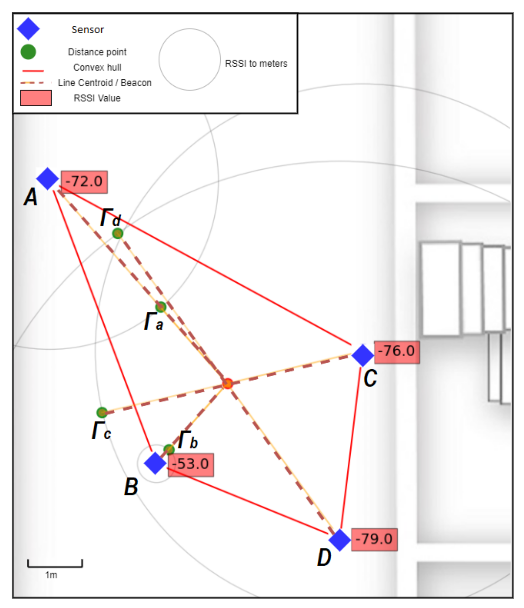
Figure 5 show a visual representation of an execution step, where ${\Gamma }_a$, ${\Gamma }_b$, ${\Gamma }_c$ and ${\Gamma }_d$ are respectively the distance points from sensor A, B, C and D. The figure shows the step between execution n = 0 and n = 1 found in Figure 6.

4. Results

4.1. Datasets Used

In this section, two datasets have been used. On each of those datasets, we used the same data processing architecture as explained in Section 2.

DS1: The first dataset is an open access dataset made by Mehdi Mohammadi et al., 2017 [24]. This dataset is composed of BLE RSSI values emitted by 13 iBeacons and the actual position of the user. As this dataset has a ground truth, it allows us to compute the accuracy value of our method. DS1 has a “grid” placement.

Table 1. Description of DS1.

Number of Sensors	Number of Instances	Placement	Duration	Frames
13	1420	Grid	8m33	33

is a description of the dataset. The number of instances is the number of RSSI values for all sensors.

The limited number of instances from this dataset forces us to use a time window size of 15 s. Indeed, to validate our approach we need at least 3 sensors returning an RSSI value between the interval of time. This leaves us with 8 min and 33 s of data to process which is limited but, the ground truth is a precious data, especially from an open access dataset.

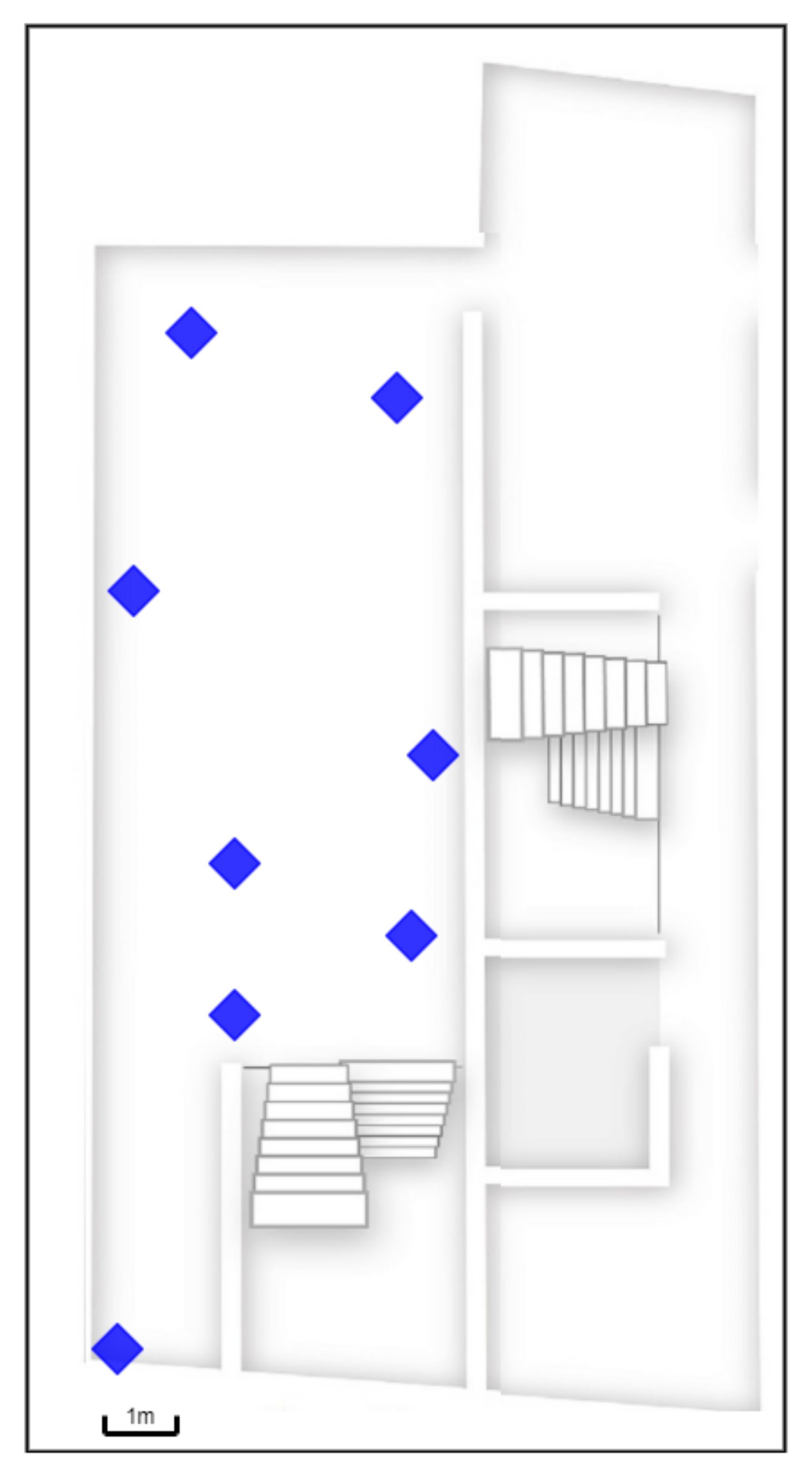
DS2: The second dataset is made of data collected during the museum experimentation. This experimentation of indoor positioning held within the museum of natural history of La Rochelle. As museums are usually closed due to the pandemic, the experimentation took place during a visit by students from a local high school.

Figure 7 describe sensor placement within the museum. We equipped the largest room in the building, and we get positional data when visitors were within this room. The experiment began at ten in the morning and ended at noon. During those two hours, subjects of the experimentation visited the museum freely. We do not have ground truth, as this is not a dataset made and controlled by our team in our office, but “on the field”, and following visitors could have changed their behavior. Finally, the three trajectories of visitors where build based on 82,630 Bluetooth total footprints collected and process with the methodology explains earlier, except we only consider intervals of time with a mean RSSI value of at least −90 dB as explained in Section 2.

Table 2. Description of DS2.

Number of Sensors	Total Number of Instances	Placement	Number of Subjects
8	82,630	Disorganized	3

show the number of sensors used, the total number of instances, the type of placements and the number of subjects.

Table 3. Description of subjects for DS2.

Tag Number	Number of Instances	Duration in Studied Room
5	26,701	16 min
8	31,403	22 min
3	24,414	3 min

show a description of three subjects from our experimentation. We should note that the number of instances is not an indicator for the time spent in the studied rooms as show tag number 3, where from 24,414 instances, we only got 3 min of exploitable data (3 sensors sending an RSSI value greater than −90 in the same time window).

4.2. Experimentation on DS1

4.2.1. Visual Representation of MZS and the Ground Truth

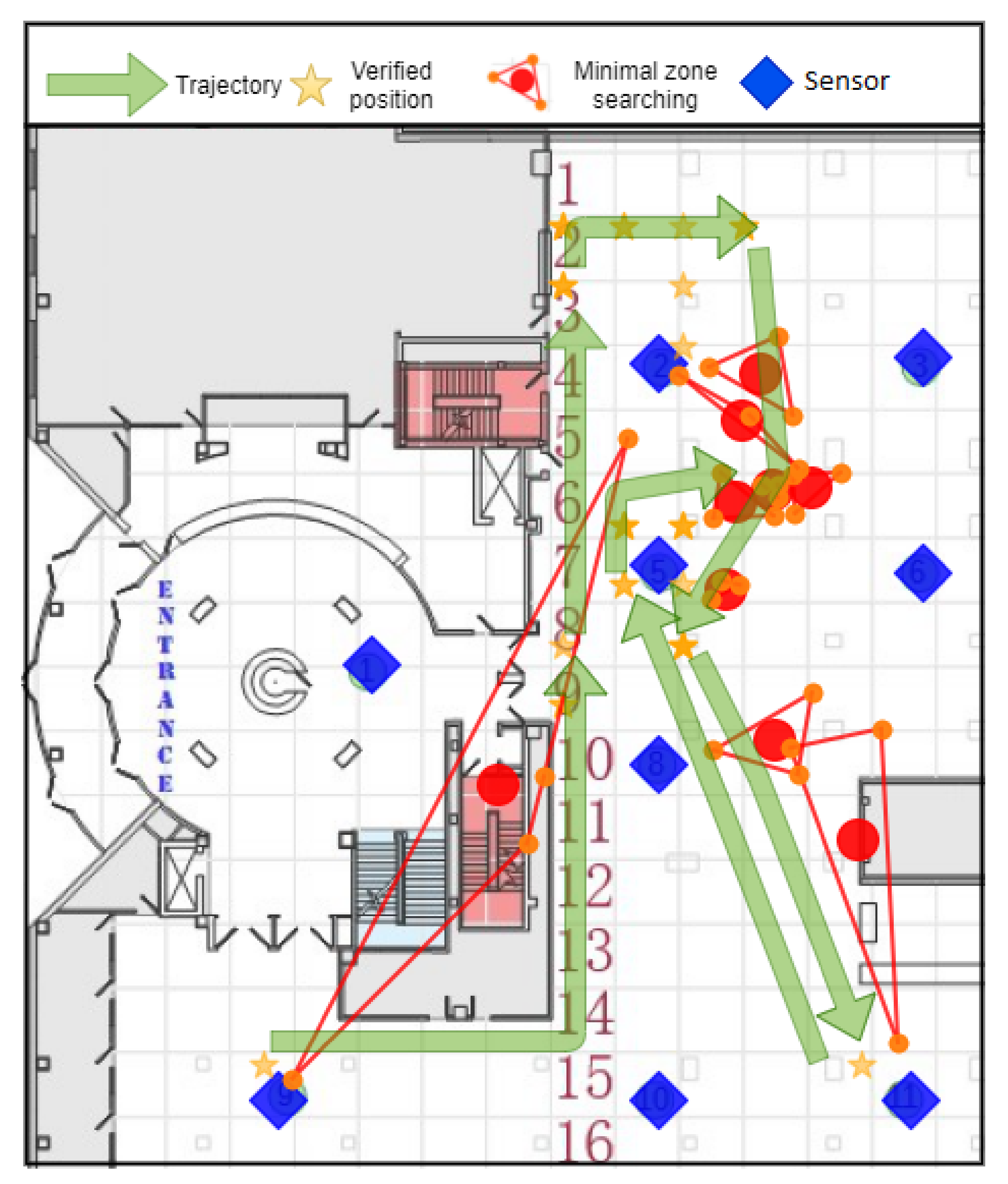
Figure 8 show a visual representation of the MZS algorithm on a “small portion” of DS1. This “small portion” is composed of 15 frames fused together (4 min), in order to better see the results returned by the MZS algorithm. The trajectory is deduced from the reference point given by the author

4.2.2. Comparison between MZS and Triangulation

The ground truth from DS1 allows us to compute an accuracy indicator. The accuracy parameter is computed by calculating the Euclidean distance from the returned zone to all verified position points each 15 s, as we can have several points of this type per interval of time. If the zone includes the point, the precision is set to 0.

Table 4. Accuracy values for MZS algorithm and triangulation applied to DS1.

Method	Accuracy	Average for Zone Size	Standard Deviation for Zone Size	Frames Computed
MSZ	0.74 m	0.49 m${}^2$	0.85	25
Triangulation	0.53 m	1.21 m${}^2$	0.95	19

shows the accuracy parameter computed for triangulation and MZS, the average and the standard deviation of size of calculated areas. The “frames computed” column of Table 4 refers to the number of position estimation that could be computed.

We can deduce that a typical “grid positional” arrangement of sensors is more suitable for the triangulation as the accuracy is better than MZS.

But we will see later that this method is vulnerable when the position of the sensors are not ideal. This validation process shows that our algorithm still gives a pretty good idea of the position of the user, even with an open access dataset.

4.3. Experimentation on DS2

Importance of the Sensor Positions

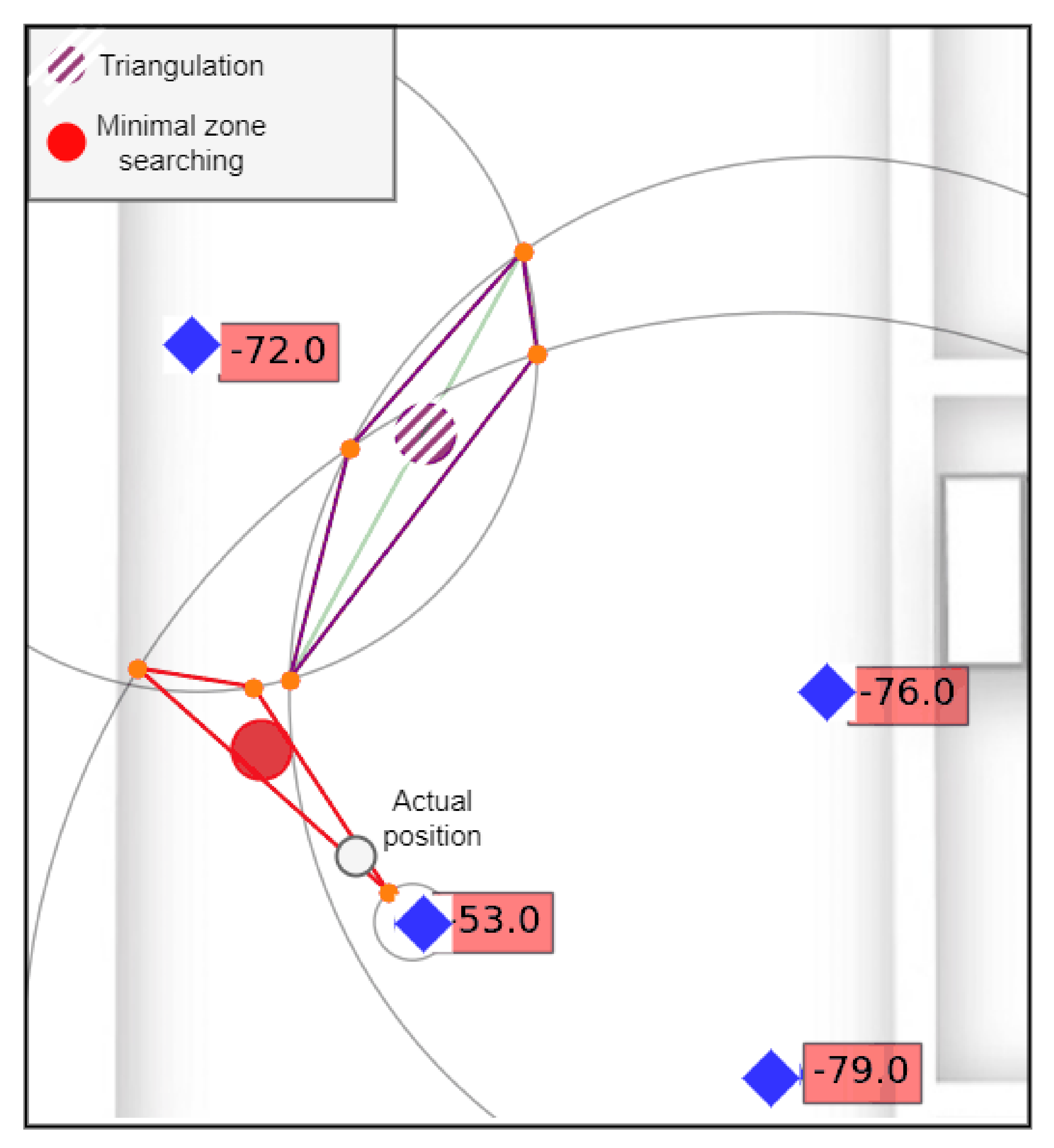
The MZS have, as it does not seek intersections between circles, a better accuracy in often case when sensor placement is not optimal. Figure 9 show a situation when the triangulation method doesn’t give the best result. The RSSI value is displayed next to the sensor and the circle around them represent the value in meter of the RSSI value collected by each sensor. It is a good example of how the sensor with the greatest value of RSSI, (and thus indicate that a person is nearby) won’t intersect with any circle making the triangulation method difficult.

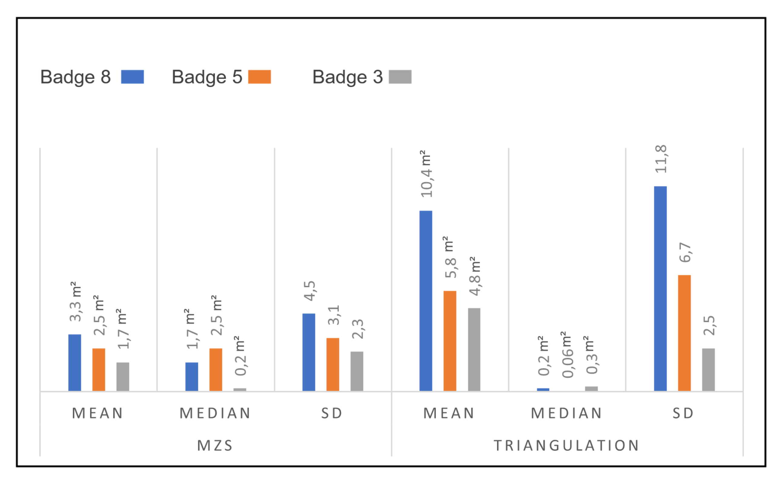
Figure 10 show the property of areas computed by both methods. This figure is a result of the museum experimentation and is built based on three visitors wearings tags 5, 8 and 3. In this figure, we are looking at the size of areas with three metrics, the mean size of the zone computed, the median and the standard variation (SD).

Table 5. Number of frames processed by MZS and the triangulation.

Badge	MZS	Triangulation	Total Number of Frames
5	181	135	194
8	254	200	263
3	24	5	31

show on how many frames both methods could have been computed. A frame is an interval of time of 5 s, where at least 2 sensors are returning an RSSI value and thus that a person is in the equipped room.

In Table 5, we see that with tag number 5, 194 frames satisfy those conditions (Meaning that this visitor spend approximately at least 16 min within the room). Tag number 8 get 263 exploitable frames (22 min) and tag number 3 get 31 meaning that the visitor probably quickly passes this room.

5. Discussion

With this information in mind, Table 5 shows that the MZS algorithm is able to return a positional area in most of the frames observed, more than the triangulation technique. Also, the MZS gives a more stable result, with a lower value of standard variation. However, The triangulation technique returns a smaller zone in comparison when we take the median. The triangulation technique certainly targets a more accurate position of the user when the target is stationary and unable to work properly when the subject is moving during the five seconds intervals. Also, the position of sensors within the room is not optimized for the triangulation algorithm and may play a big part in those results as situations describe in Figure 9 lead to poor performances.

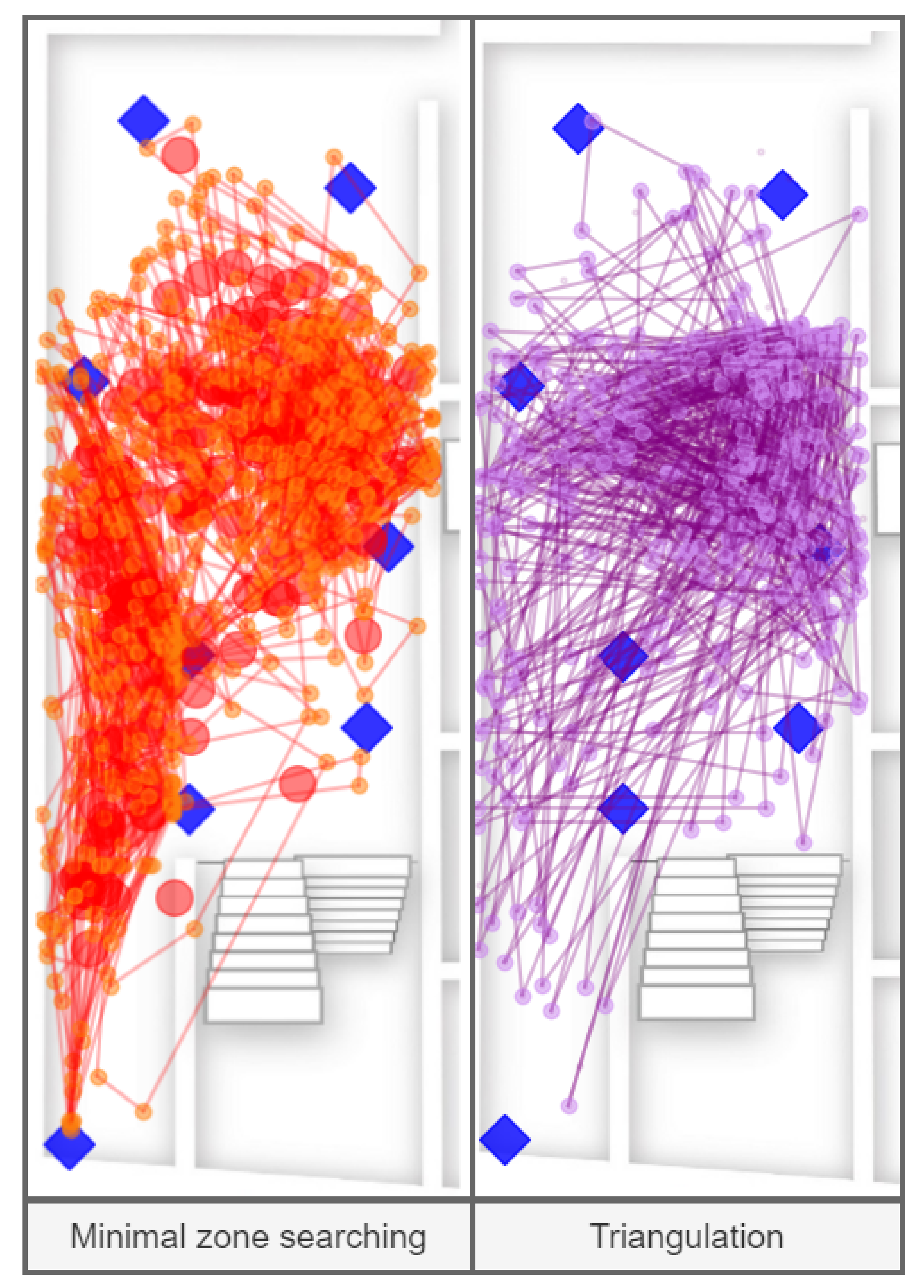
In Figure 11 we show a visual representation of areas computed by both methods and held as an illustration of data from Table 5 and more precisely the tag number 8. All areas computed by those two algorithms are printed together on the same picture.

The MZS algorithm shows his strength on this figure: The localisation of the visitor in the center of the room show comparable result between the two methods, but the difference stand in the center to bottom left of the room. We see that the triangulation method show poor result in tight spaces, where only few sensors are reachable. And thus, results returned by the MZS algorithm are more exploitable and give a more meaningful view on the visit of the subject.

6. Conclusions

Indoor positioning services apply to museums offer new and promising ways to study visitor behaviors. It can help the management of such facilities, in order to monitor visitor paths and see what are the pieces they admire the most and what are the ones they miss. Indeed, managers of museums are always looking for new ways to improve the visiting experience, and are often worried that we will miss something during the tour.

But those kind of place also bring architectural constrains in sensor placement, and as we saw, sometime making algorithms such as the triangulation less effective. The MZS algorithm in other hand, as promising results as the position of sensors seems to have less impact, making it specifically useful in tight spaces. This kind of indoor positioning technique is still in an early stage of development, and improvement can still be made. An area for improvement can be the use of additional technique, such as trilateration, to reduce the tracking error. As the MZS algorithm seeks to get a zone and thus can be taken into account with another method, but if used alone, only return a zone, making accurate positional representation difficult. Sensor placement can indeed have a huge impact on accuracy and performances on various techniques, and it’s something that should be considered more carefully as studies shown [25,26].

BLE remains a reference signal in the field of indoor positioning and make experimentation as the one described in this paper easier and do not need a lot of materials to be efficient and can alone give a rough idea of the position of a visitor, even in real time.

Finally, we can also add that indoor positioning systems in most cases do not need a complex algorithm, often too heavy to be processed by a smartphone or too difficult to implement. Studies such as [27,28,29], shows in different ways the use of the architecture and room’s layout of a building. Thus, the search for maximum accuracy become less relevant, when we know where the user can and cannot be, and what path could he follow. Therefore, the robustness of a method should be more valuable than its accuracy.

References

- Zafari, F.; Gkelias, A.; Leung, K.K. A Survey of Indoor Localization Systems and Technologies. IEEE Commun. Surv. Tutor. 2019, 21, 2568–2599. [Google Scholar] [CrossRef] [Green Version]
- Piccinni, G.; Avitabile, G.; Coviello, G. An improved technique based on Zadoff-Chu sequences for distance measurements. In Proceedings of the 2016 IEEE Radio and Antenna Days of the Indian Ocean (RADIO), Reunion, France, 10–13 October 2016; pp. 1–2. [Google Scholar] [CrossRef]
- Piccinni, G.; Avitabile, G.; Coviello, G.; Talarico, C. Real-Time Distance Evaluation System for Wireless Localization. IEEE Trans. Circuits Syst. I Regul. Pap. 2020, 67, 3320–3330. [Google Scholar] [CrossRef]
- Luo, R.C.; Hsiao, T.J. Dynamic Wireless Indoor Localization Incorporating With an Autonomous Mobile Robot Based on an Adaptive Signal Model Fingerprinting Approach. IEEE Trans. Ind. Electron. 2019, 66, 1940–1951. [Google Scholar] [CrossRef]
- Farid, Z.; Nordin, R.; Ismail, M. Recent Advances in Wireless Indoor Localization Techniques and System. J. Comput. Netw. Commun. 2013, 2013, 185138. [Google Scholar] [CrossRef]
- Liu, H.; Darabi, H.; Banerjee, P.; Liu, J. Survey of Wireless Indoor Positioning Techniques and Systems. IEEE Trans. Syst. Man Cybern. Part C (Appl. Rev.) 2007, 37, 1067–1080. [Google Scholar] [CrossRef]
- Conte, G.; de Marchi, M.; Nacci, A.A.; Rana, V.; Sciuto, D. BlueSentinel: A first approach using iBeacon for an energy efficient occupancy detection system. In Proceedings of the 1st ACM Conference on Embedded Systems for Energy-Efficient Buildings (BuildSys’14), Memphis, TN, USA, 3–6 November 2014; Association for Computing Machinery: New York, NY, USA, 2014; pp. 11–19. [Google Scholar] [CrossRef]
- Yoshimura, Y.; Sobolevsky, S.; Ratti, C.; Girardin, F.; Carrascal, J.P.; Blat, J.; Sinatra, R. An Analysis of Visitors’ Behavior in the Louvre Museum: A Study Using Bluetooth Data. Environ. Plan. B Plan. Des. 2014, 41, 1113–1131. [Google Scholar] [CrossRef] [Green Version]
- Spachos, P.; Plataniotis, K.N. BLE Beacons for Indoor Positioning at an Interactive IoT-Based Smart Museum. IEEE Syst. J. 2020, 14, 3483–3493. [Google Scholar] [CrossRef] [Green Version]
- Giuliano, R.; Cardarilli, G.C.; Cesarini, C.; di Nunzio, L.; Fallucchi, F.; Fazzolari, R.; Mazzenga, F.; Re, M.; Vizzarri, A. Indoor Localization System Based on Bluetooth Low Energy for Museum Applications. Electronics 2020, 9, 1055. [Google Scholar] [CrossRef]
- Juniarta, N.; Couceiro, M.; Napoli, A.; Raïssi, C. Sequential Pattern Mining using FCA and Pattern Structures for Analyzing Visitor Trajectories in a Museum. In Proceedings of the CLA 2018—The 14th International Conference on Concept Lattices and Their Applications, Olomouc, Czech Republic, 12–14 June 2018. [Google Scholar]
- Kontarinis, A.; Marinica, C.; Vodislav, D.; Zeitouni, K.; Krebs, A.; Kotzinos, D. Towards a Better Understanding of Museum Visitors’ Behavior through Indoor Trajectory Analysis. In Proceedings of the Seventh International Conference on Digital Presentation and Preservation of Cultural and Scientific Heritage (DiPP2017), Burgas, Bulgaria, 7–9 September 2017; pp. 19–30. [Google Scholar]
- Belmonte-Hernández, A.; Hernández-Peñaloza, G.; Gutiérrez, D.M.; Álvarez, F. SWiBluX: Multi-Sensor Deep Learning Fingerprint for Precise Real-Time Indoor Tracking. IEEE Sens. J. 2019, 19, 3473–3486. [Google Scholar] [CrossRef]
- Wenger, M.; Carrera, J.; Zhao, Z. Indoor positioning using Raspberry Pi with UWB. Bachelor’s Thesis, Universität Bern, Bern, Switzerland, 2019. [Google Scholar]
- Choi, M.; Beakcheol, J. An accurate fingerprinting based indoor positioning algorithm. Int. J. Appl. Eng. Res. 2017, 12, 86–90. [Google Scholar]
- Subedi, S.; Kwon, G.; Shin, S.; Hwang, S.; Pyun, J.Y. Beacon based indoor positioning system using weighted centroid localization approach. In Proceedings of the 2016 Eighth International Conference on Ubiquitous and Future Networks (ICUFN), Vienna, Austria, 5–8 July 2016; pp. 1016–1019. [Google Scholar] [CrossRef]
- Dong, Q.; Dargie, W. Evaluation of the reliability of RSSI for indoor localization. In Proceedings of the 2012 International Conference on Wireless Communications in Underground and Confined Areas, Clermont-Ferrand, France, 28–30 August 2012; pp. 1–6. [Google Scholar] [CrossRef] [Green Version]
- Li, G.; Geng, E.; Ye, Z.; Xu, Y.; Lin, J.; Pang, Y. Indoor Positioning Algorithm Based on the Improved RSSI Distance Model. Sensors 2018, 18, 2820. [Google Scholar] [CrossRef] [PubMed] [Green Version]
- Wang, Y.; Yang, X.; Zhao, Y.; Liu, Y.; Cuthbert, L. Bluetooth positioning using RSSI and triangulation methods. In Proceedings of the 2013 IEEE 10th Consumer Communications and Networking Conference (CCNC), Las Vegas, NV, USA, 11–14 January 2013; pp. 837–842. [Google Scholar] [CrossRef]
- Pradhan, S.; Bae, Y.; Pyun, J.Y.; Ko, N.Y.; Hwang, S. Hybrid TOA Trilateration Algorithm Based on Line Intersection and Comparison Approach of Intersection Distances. Energies 2019, 12, 1668. [Google Scholar] [CrossRef] [Green Version]
- Cantón Paterna, V.; Calveras Augé, A.; Paradells Aspas, J.; Pérez Bullones, M.A. A Bluetooth Low Energy Indoor Positioning System with Channel Diversity, Weighted Trilateration and Kalman Filtering. Sensors 2017, 17, 2927. [Google Scholar] [CrossRef] [PubMed] [Green Version]
- He, S.; Hu, T.; Chan, S.-H.G. Contour-based Trilateration for Indoor Fingerprinting Localization. In Proceedings of the 13th ACM Conference on Embedded Networked Sensor Systems (SenSys’15), Delft, The Netherlands, 6–8 November 2015; Association for Computing Machinery: New York, NY, USA, 2015; pp. 225–238. [Google Scholar] [CrossRef]
- Dinh, T.-M.T.; Duong, N.-S.; Sandrasegaran, K. Smartphone-Based Indoor Positioning Using BLE iBeacon and Reliable Lightweight Fingerprint Map. IEEE Sens. J. 2020, 20, 10283–10294. [Google Scholar] [CrossRef]
- Mohammadi, M.; Al-Fuqaha, A.; Guizani, M.; Oh, J. Semi-supervised Deep Reinforcement Learning in Support of IoT and Smart City Services. IEEE Internet Things J. 2017, 5, 624–635. [Google Scholar] [CrossRef] [Green Version]
- Rezazadeh, J.; Subramanian, R.; Sandrasegaran, K.; Kong, X.; Moradi, M.; Khodamoradi, F. Novel iBeacon Placement for Indoor Positioning in IoT. IEEE Sens. J. 2018, 18, 10240–10247. [Google Scholar] [CrossRef]
- Sharma, R.; Badarla, V. Geometrical Optimization of A Novel Beacon Placement Strategy for 3D Indoor Localization. In Proceedings of the 2018 IEEE International Conference on Advanced Networks and Telecommunications Systems (ANTS), Indore, India, 16–19 December 2018; pp. 1–6. [Google Scholar] [CrossRef]
- Ramadhan, H.; Yustiawan, Y.; Kwon, J. Applying Movement Constraints to BLE RSSI-Based Indoor Positioning for Extracting Valid Semantic Trajectories. Sensors 2020, 20, 527. [Google Scholar] [CrossRef] [PubMed] [Green Version]
- Abdelnasser, H.; Mohamed, R.; Elgohary, A.; Alzantot, M.F.; Wang, H.; Sen, S.; Choudhury, R.R.; Youssef, M. SemanticSLAM: Using Environment Landmarks for Unsupervised Indoor Localization. IEEE Trans. Mob. Comput. 2016, 15, 1770–1782. [Google Scholar] [CrossRef]
- Kontarinis, A.; Zeitouni, K.; Marinica, C.; Vodislav, D.; Kotzinos, D. Towards a semantic indoor trajectory model: Application to museum visits. Geoinformatica 2021, 25, 311–352. [Google Scholar] [CrossRef] [PubMed]