Abstract
A technique employed by recommendation systems is collaborative filtering, which predicts the item ratings and recommends the items that may be interesting to the user. Naturally, users have diverse opinions, and only trusting user ratings of products may produce inaccurate recommendations. Therefore, it is essential to offer a new similarity measure that enhances recommendation accuracy, even for customers who only leave a few ratings. Thus, this article proposes an algorithm for user similarity measures that exploit item genre information to make more accurate recommendations. This algorithm measures the relationship between users using item genre information, discovers the active user’s nearest neighbors in each genre, and finds the final nearest neighbors list who can share with them the same preference in a genre. Finally, it predicts the active-user rating of items using a definite prediction procedure. To measure the accuracy, we propose new evaluation criteria: the rating level and reliability among users, according to rating level. We implement the proposed method on real datasets. The empirical results clarify that the proposed algorithm produces a predicted rating accuracy, rating level, and reliability between users, which are better than many existing collaborative filtering algorithms.
1. Introduction
Due to the growth of websites and e-commerce sites, online users and items have increased substantially. As a competitive operation, e-commerce requires obtaining solutions that may help to improve sales, competitive advantages, and customer satisfaction. Recommendation systems (RS) aid these marketplaces by providing customers with recommendations based on their prior preferences. As a result, recommendation algorithms are commonly coupled with various domains of knowledge [1].
Based on earlier studies, RSs can be classified into the following types [2]: collaborative filtering (CF), content-based filtering (CB), demographic filtering (DF), knowledge-based filtering (KB), and hybrid. The most common methods for recommending items to users are based on CF [3]. Typically, CF algorithms are categorized into user-based and item-based models [4]. In the user-based CF algorithm, recommender systems collect similar users into groups and recommend highly-rated items to similar users [5]. On the other hand, in the item-based CF system, the similarity between objects is determined based on the items’ ratings. Then, groups of similar items can be created. Finally, if a user rated a specific item highly, similar items might be recommended [6].
Despite numerous studies and analyses on the user–user and item-item CF similarity measures, these measures do not infer sufficient similarity in some cases. Traditional CF algorithms offer recommendations only user ratings for items, regardless of the effects that many features on user similarity [7] and item similarity [8]. Therefore, it is essential to find a similarity measure based on the actual preferences of users rather than user rating values. Therefore, researchers are considering the effect of item characteristics on the recommendation accuracy of RSs [9,10,11]. A model that mixes item-based CF information content was introduced in [12]. The authors created a clustering method based on mixed information. The k-mean clustering model and weighted deviations were used to determine the closest neighbors, and then the rating prediction for unrated items was calculated. In [13], the authors formed a special RS by analyzing the item genre relationship and user-preferred genres. The Pearson correlation coefficient (PCC) and clustering approaches were used to calculate genre similarity. Then, the model can suggest a recommended genre to an active user.
However, CF algorithms suffer from several drawbacks, and the common ones are data sparsity and user cold-start. Data sparsity intimates an insufficient number of ratings for items from users; sparseness in the <user x item> matrix, limiting the CF algorithm’s ability to pick a suitable set of similar users [14,15,16]. In parallel, the cold-start problem is a significant issue in recommender systems; this problem is divided into cold users and cold items. The problem with cold users occurs due to a lack of information about the user’s preferences [15,17]. Depending on the CF, a user cannot receive any recommendations from the system [18,19]. An increased number of new users and multiple less-active users joining e-commerce sites in all applications cause real problems for the existing recommendation algorithms [20]. At the same time, the problem with cold items occurs from the lack of ratings for a new item [15,17]. Acceptable recommendation quality cannot be obtained when little or no information is available [21].
Recent literature indicates that many RS problems have been approached through various hybrid methods, including side information to determine user interests and purchasing habits [22]. A previous study [23] presented a method based on exploiting collaborative tagging as supporting information to extract users’ tastes for items. Their research overcame the user cold-start and sparsity problems.
Regardless of the many solutions proposed to solve the user cold-start and sparsity problems, such as those in [16,24,25,26,27], most of these solutions rely only on user ratings rather than actual user preferences for items. Therefore, there is indeed a deficiency in features upon which user similarity is determined. Similarity metrics should not be limited to user ratings of specific items or matching their primary demographic data. There is a pressing need to examine additional and diverse features that adequately describe individuals across several domains.
In this paper, the fundamental objective is to create a new similarity measure by finding the similarity between users based on preferred-item genres. It, furthermore, enhances the prediction accuracy of RSs, even for customers who leave few ratings.
1.1. Problem Definition
According to research [24], user preferences are not fixed and indicate constant fluctuations in their preferences for items. Hence, it is not easy to find a similarity method that matches all user behaviors. The user similarity measure based on the item genre is not widely explored in RSs. Furthermore, traditional similarity measures do not make accurate recommendations for new users or items, and they are less effective with sparse datasets [16,25]. Initially, a precise similarity measure can be configured between users depending on a user’s preferences for an item’s genre. Basing on movie lens [26] and Yahoo Music datasets, our research experiments looked at user preference for movie/music genres. Some movies have multiple genres (see Figure 1); two users, u1 and u2, are highly similar in terms of their choices and ratings of action, fantasy, adventure, and horror. At the same time, they are different in their choices in terms of comedy and drama movie genres. This is, consequently, related to their personalities.
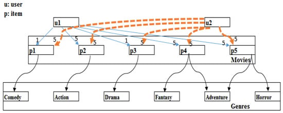
Figure 1.
Example of user preferences for movie genres.
Traditional similarity algorithms hold all u1 and u2 ratings collectively. Calculating their similarity shows that their relationship is medium because of their remarkable similarity for action, fantasy, adventure, horror movie genres, and the weak similarity between comedy and drama. Hence, the results fail to show that their preferences for many movie genres are notably significant and are reasonably soft for the other genres. Thus, the traditional similarity algorithms are incapable of representing the different choices of multiple-interest users. Furthermore, a similar rating might not mean similarity in terms of actual preferences. Therefore, relying solely on user ratings may produce incorrect similarity between users or items. A user can frequently imagine the story and spirit of a movie according to that movie’s genre(s); thus, a movie’s genre helps to attract a user’s attention to decide whether or not to see that movie [9]. Accordingly, extracting critical choices and contextual information from user profiles is essential to establish vital similarity metrics among users. Therefore, we aimed to solve this problem.
1.2. Novelty
Many datasets; like movie lens data set; are sparse [27,28], efficient solutions should avoid this problem and not rely entirely on user ratings. Therefore, to increase the recommendation accuracy and overcome the data sparsity problem, a user-based similarity model according to user preference for an item’s genre has been suggested. The novelty of the proposed similarity measure is represented by measuring a user’s average preference for a specific genre. Firstly, we calculated the average of the active user ratings for items in their preferred genres; secondly, user similarity was computed by comparing average user preferences across genres. Then, by specifying a target user’s initial neighbors in each genre, based on a certain similarity threshold with other users, we can create the target user’s initial neighbors list. Finally, users who shared the target user’s tastes across all preferred genres were extracted and the target user’s final neighbors list was made.
1.3. Paper Contribution
This research aims to find users’ similarity measures based on their preferences for item genres, even for users who only leave a few ratings. The essential contributions of this article are:
- Suggesting user similarity measures according to their general preferences for item genres;
- Proposing new evaluation criteria: the level of predicted ratings and users’ reliability;
- Preparing a detailed analysis to verify our presumption that the suggested model exceeds the current CF algorithms in prediction accuracy.
The remainder of the article is structured as follows. Section 2 reviews studies related to our method. The background of our suggestions is described in Section 3. Section 4 briefly explains the proposed model, while Section 5 presents the conducted experiment. Finally, in Section 6, we provide the conclusions of the study and ideas for future work.
2. Related Work
RSs use filtering methods to acquire information on entities (i.e., users or items). Therefore, the researchers provided many similarity measures for CF–RSs to establish a recommendation’s accuracy at the necessary level. Utilizing entity-side information is a frequently used technique for resolving RS issues and obtaining appropriate recommendations [22]. In the following, we summarize some of the studies that used entities’ side information to enhance RS accuracy.
In [25], the authors used location information in recommendation algorithms to create a mobile learning application focused on presenting users with favorable recommendations. At the same time, the authors of [29] planned differently to increase the accuracy of RSs. They suggest approach that based on the addition of contextual information to establish relationships between users or products. As a result, they suggested many mathematical methods for information filtering and modeling, which demonstrated through experimental results that contextual information is critical for receiving correct recommendations.
Following this, item genres were incorporated into an RS to increase the RS’s accuracy. Several studies have concentrated on utilizing the movie genre feature to collect user input and enhance suggestions, particularly for massive datasets [30,31]. Others improved an RS called “Taste Weights” [32]; analyzing a user’s Facebook profile identified their preferred music genre. Then, the semantic web resource “DB pedia” was utilized to discover new artists performing music in the same genre as the active user’s favorite. Such music was recommended to other users. The authors of [33] presented a music recommendation system that uses users’ behavioral features in the model and exploits a user’s overall mood and sentiment to produce recommendations. In addition, they blended CB recommendations with user personality qualities on social networking sites, behavior, interests, and requirements and examined several methods for inferring user personality qualities. In [28], a genre-based algorithm was developed using the notion of item genres rather than the items themselves. The algorithm picked neighbors based on their genre preference, comparable to those of others in the community. This research used user data to determine item similarity, and CF sparsity was alleviated. In [34], a clustering method using an item’s genre information was presented. This model focuses on establishing a hybrid approach, combining the CB clustering method and CF, instituted by the item genre’s investment. The model improved the rating prediction operation with a less time-consuming model. Differently, in [35], the authors introduced a user similarity model based on genre preferences to present a weighted link prediction model according to complex network modeling and a detected user community.
Researchers have continued to exploit item genres to create a recommender system; in [36], novel user-based similarity measures based on a vector to hold user similarity using item genres was presented. The model finds the global, local, and meta similarities between users to create a similarity vector and reveals and estimates user associations under different scenarios. They emphasized that user similarities might be defined differently depending on the various item genres.
The work in [37] focused on employing item genres to raise predicted rating accuracies and overcome the sparsity problem. The algorithm involves creating a matrix containing the user’s item weight by combining two vectors. The first vector is the user’s taste vector, extracted from the user’s ratings for items. The second vector contains the degree of items belonging to a specific type, which results from the exploitation of the collective ratings of a particular item. Finally, the resulting matrix was used to get the prediction of the desired item.
Researchers used trust information to improve prediction accuracy and overcome cold-start and sparsity problems. In [38], two approaches were presented for calculating user trust in items according to their ratings. Although it is challenging to obtain trust information between users and objects, the proposed method performed better than tested methods in addressing the specific problems.
The accuracy and quality of recommender systems diminish when entity information is insufficient [21]. Therefore, various solutions have been proposed to solve the sparsity and cold-start problems. The study in [39] introduced a hybrid approach for solving sparse data by determining user interests. The movie feature was used to create a vector of movie attributes and was merged with the user rating vector to generate a user interest vector to calculate user similarity. As a result, this method outperformed specific existing recommendation algorithms in terms of accuracy. The authors of [40] enhanced prediction accuracy by using auxiliary data on a user’s demography and item characteristics. The model incorporates supervised label terms to make feasible recommendations for new entities using a matrix factorization framework. In [41], a method for resolving the cold-start status using a clustering approach was proposed. This approach was constructed using a user’s preferred item ratings and genres to determine similarity. The results demonstrated that the suggested model could significantly improve the cold-start solution and outperform comparable approaches in standard recommendations and cold-start situations. However, new users may abandon the system due to flaws in the suggestions during the initial phases when users lack the necessary ratings to needed by the CF in RS to calculate their user similarity. To address this issue, the authors of [42] proposed implementing a neural learning-based user similarity measure that would deliver favorable recommendations to users with few ratings (2 to 20 ratings). The experimental results demonstrated that this system was more precise, recallable, and accurate than its predecessors.
Unlike algorithms that only rely on user ratings, we seek to develop a similarity measure that incorporates user interest and identifies user-suitable neighbors, even when they leave very few ratings. Since specialists in the relevant item fields handle item genre information, the genre is regarded as reliable information that can be used to identify user similarities. The proposed technique computes users’ average preferences for each item genre. Then, it identifies nearest neighbors in each genre, based on a similarity threshold value. Finally, by intersecting user preferences per genre, it determines neighbors who share the same tastes across all genres and considers them the ultimate neighbors for the current user. We applied our method to real datasets and performed different experiments to verify the suggested method’s accuracy and efficacy in picking correct neighbors. Our novel approach consistently generated superior results, even for users with a few ratings compared to past baseline procedures.
3. Background
3.1. Memory-Based Algorithm
As illustrated in Figure 2, current recommendation algorithms can be classified into four types: CB, CF, KB, and hybrid [43], CF is the most common technique amongst them and is either memory-based or model-based [3]. We analyzed the memory-based approach based on early user ratings for an item arranged in a rating matrix. The neighbor-based algorithm is the most well-known algorithm of the memory-based process. It predicts ratings based on users’ ratings that are similar to the active user. There are two neighbor-based algorithms: users-based CF [43] and item-based CF [8]. In this paper, we analyzed the user-based CF class. Ordinarily, the two essential steps in CF algorithms are: selecting proper neighbors according to a similarity measure and predicting the rating to generate recommendations for an active user [44]. There are various similarity measures, such as PCC [8] and mean-squared difference [45]. As an output, the similarity method produces a user similarity matrix, determining the similarity or correlation between user pairs. Thus, building a similarity between users forms the necessary neighborhood. Then, a rating of unrated items is predicted using various procedures [46,47]. The technique used in this paper is explained in Section 3.2.
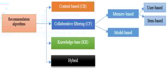
Figure 2.
Current recommendation algorithms and categories.
3.2. Rating Prediction
Rating prediction calculation is a standard significant action in CF-based algorithms [8]. After identifying an active user’s neighbors, the ratings of an active user a of item p can be expected based on the ratings of his neighbors. Researchers have proposed several prediction methods that have been widely used in recommendation systems [46,47]. In our research, we relied on the prediction method suggested in [48]. This prediction method was based on the first available rating from the active user’s closest neighbor (K-NN). Assuming that I = {p1, p2…m} is a set of common items, the user-based model prediction formula is explained in the following Equation (1):
where:
- : Is the predicted rating value for unrated item pi.
- : is u′s rating value for pi.
- : represents the K nearest neighbor set of and RRepresents items rated by u. Then, after giving a detailed summary of the background and rendering the broad forms of collaborative filtering, we present our offered similarity measure in the next section.
4. Proposed Model
A user-based relationship analysis model has been offered based on item genres. However, current CF-based approaches cannot suggest items for users with acceptable accuracy when dataset sparsity is high. Therefore, they offer undesirable recommendations, in particular, for users with a few ratings. To rectify this issue, we aimed to define the relationship between users by exploiting item genre information, which appears confident in terms of robust relationship measurements with reasonable error values in the sparse dataset.
As explained before, examining only user ratings to find similarities between users does not consistently deliver accurate recommendations. Two users might rate the same movie with the same rating for multiple reasons, which differ from each other, for example due to liking the movie genre or because they prefer the movie’s actor, or other reasons. Therefore, the similarity method must expose actual user preferences.
4.1. User-Based Similarity Measure Using Item Genre Information
This section includes a user-based similarity measure model, defined from user preferences for item genres. In this model, the classifications of users were prepared according to their preferences for item genres. Then, the similarity between users was determined according to the average user rating for the item genres, thus it was named the user–genre similarity model (UGSM), and is shown in Figure 3.
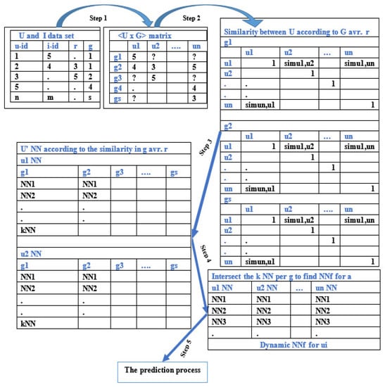
Figure 3.
Proposed model flowchart.
As a result of classifying users according to their favorite item genres, we constructed Table 1, showing a representative sample of five users and their preferred genres. Assuming that U = {u1, u2…un} represents the set of users, and G = {g1, g2…gs} represents the collection of genres, and I = {p1, p2… pm} is a set of common items, the item genres in Table 1 refer to the movie genres identified in the movie lens dataset [26], and the values represent the average user ratings for their preferred genres.

Table 1.
Users (u) and their mean rating on preferred item genres (g).
From Table 1, it is clear that an item may be related to multiple genres and that user preferences differ from one genre to another. Selecting an active user (a) of a particular genre means the user prefers that genre. Therefore, there are remarkable opportunities for two users to be highly similar when they like the same genre. The essence of memory-based CF algorithms is calculating the actual similarity between entities to select proper neighbors. Thus, in addition to the rating prediction phase, the proposed similarity measure involves four significant steps:
- Step 1: Building a genre rating <u × g> matrix from the master dataset, including (u-id, i-id, r, i-g) by calculating the user preference average per item genre (g).
- Step 2: Finding the similarity between the users’ preferences per genre using Equation (2). A slight difference indicates a significant similarity.
- User’ similarity is calculated as the absolute difference between user rating average for the same genre.
- Step 3: Finding the nearest neighbors (K-NN) for each user per genre by arranging the difference values in the preferences rate in ascending order.
- Step 4: Finding the final nearest neighbors (NNf) for the active user by intersecting the groups of K-NN in the previous step to get the neighbors who share all their preferences with the active user, according to Equation (3).
As shown in Table 1, if two users are similar to each other in terms of their preferences for a genre, they may differ for different genres. Therefore, the similarity model must carefully choose a similar neighbor to in terms of their preferences for genres. Accordingly, the UGSM includes an intersection process among the first K-NN in all genres to find ′s closest neighbors, similar to in all preferences.
Each will have several neighbors, which differ from other s. The reason for this is that the intersection process will keep users who are similar to in all genres. Thus, the results of the intersection process for users vary from one to another. For example, the first might get 40 NNf, while the second might get only 35. If the similarity values among and many neighbors are equal, to form the these neighbors are arranged in descending order according to the number of common genres shared with . To maintain the most significant number of neighbors sharing one or more genre with the active user, the proposed model includes the following process:
- Step 5: The active user rating prediction process.
To recommend the correct item to the active user, the final step in the proposed model is active user rating prediction. The proposed model relies on the prediction model proposed in [48], which is based on the first available rating from the closest neighbors, as illustrated in Section 3.2. Then, the final neighbors’ average aggregate rating differences are ordered in descending order to establish the proper neighborhood’s ranking.
4.2. An Illustrative Example of the Proposed Algorithm
For elucidation, the following example explains the UGSM similarity measure model. Assuming that there are five users (u1, u2, u3, u4, and u5) and five genres (g1, g2, g3, g4, and g5), based on Table 1 and Equation (2), the differences in the values between the five users are shown in Table 2. We denoted the values of the differences between two users on an uncommon genre with the symbol “-”. Then, we determined the first 3-NN for u1, as shown in Table 3.
Table 2.
Differences between 5 users according to 5 preferred genres.
Table 3.
First 3-NN and NNf for u1.
Accordingly, from Table 3, for u1, the first 3-NNs in g1 are u2, u4, and u5. In g2 they are u4, u5, and u2, and so on. Therefore, based on Equation (3), the final list for u1 NN (u1 NNf) contains only u4 and u5. In the prediction process, the predicted rating will be based on u4 first because the average difference between u1 and u4 was 0.625 and with u5 it was 0.87. However, if there is an unrated item in the u4 profile, the prediction operation will be based on the u5 ratings.
4.3. Proposed Evaluation Metrics
4.3.1. Predicted Rating Level (P.L.)
Since we endeavored to improve the accuracy of RSs, we suggested a new evaluation measure, named predicted rating level determination, which divides the ratings into:
- The positive level (POS): is represented when the rating is r > (max/2); where “max” means the maximum score rating in the dataset.
- The average level (AVG): when is r = (max/2); and
- The negative level (NEG), when is r < (max/2).
We supposed that, if the predicted and original ratings were both at the same level, the proposed model’s outputs were accurate, and the model was capable of selecting an appropriate neighborhood.
4.3.2. Communities Reliability Level (Rel. L.)
We strived to quantify community reliability. As a result, we presented a new measure of reliability based on the ratio of common ratings with a similar rating level between the active user and their neighbor. For the new measure, a high value indicates high reliability. The reliability can be obtained from Equation (4):
where . The number of common item, , between and their neighbors,, which are at the same rating level,; i = 1,..., K-NN. is the rating level of and .
5. Experiments
The experiments were performed on two datasets to examine the accuracy of the outcomes when employing the suggested UGSM. The experiments included evaluating the accuracy, the level of the predicted rating, and reliability between users, in addition to the comparison of UGSM to current CF algorithms.
5.1. Datasets
To measure the effectiveness of the proposed similarity measure, we relied on an offline analysis approach based on previously collected data from websites [49]. We used two offline datasets: Movie lens (ML-20M) (https://grouplens.org/datasets/movielens/20m (2 February 2021)) [26] and R2-yahoo! Music user ratings of songs with song attributes, version 1.0 datasets (https://webscope.sandbox.yahoo.com/catalog.php?datatype=r&did=2 (15 May 2021)). The ML-20M dataset was collected by the Group Lens Research Team at the University of Minnesota. Each user had at least 20 ratings, and it included two separate files: the first file consisted of (User id, Movie id, rating) and the second file consisted of (Movie id, Movie title, Movie genre). In this dataset, 7120 users participated to rate 27,278 movies and the number of ratings was 1,048,575. Movies were classified into 20 genres. The R2-yahoo! Music dataset represented music preference data for songs from the Yahoo site. It included multiple files: the first file contained (User id, Song id, rating), the second file included (Song id, Music genre id), and the last file included (Genre id, Genre name). We used the data in the “ydata-ymusic-user-song-ratings-meta-v1_0/train-1.txt” file. This dataset contained 2829 users, 127,217 songs, and 58 music genres.
In both datasets, the files were merged to implement the proposed algorithm. We needed a user id, movie/song id, movie/music genre id, and user rating for the movie/song. Furthermore, we compared our findings to previous researchers’ findings by utilizing additional datasets (ML1 and ML-1M). The sparsity level was obtained using the following Equation (5) [50]:
where m represents the total number of users, and n represents the total number of items. In brief, our experiments were based on the first 1500 users who had the highest number of ratings (more than 100 ratings). The dataset details are shown in Table 4.
Table 4.
Data sets Detail.
Since the proposed algorithm depends on genre information, we describe the genre information in Table 5 and Table 6 for the ML-20M dataset and Table 7 for R2-yahoo! Music dataset. Table 5 shows the genre names and the number of movies that belong to them. The drama genre was the most common, and there were 13,344 drama movies. The comedy genre came in second, and there were 8374 movies. Thus, this dataset contained 246 movies belonging to the “unknown” genre, which we excluded from the dataset in the experiments.
Table 5.
Genre name in ML-20 M dataset and number of movies per genre.
Table 6.
Several g and the movies of that g in ML-20M dataset.
Table 7.
Genre name in R2-Yahoo Music dataset and number of songs per genre.
Table 6 shows the number of genres and the number of movies in that genre. The movie may belong to more than one genre. A total of 10,829 movies belonged to a single genre, while 8800 movies belonged to the complex genre (i.e., contained more than one genre). Some movies belonged to five genres.
Table 7 shows the genre name in the R2-yahoo music dataset and the number of songs that belongs to it. Most songs have an unknown “un” genre, where there are 109,890 “un” genre songs. Since we did not use any item from the “un” genre in the experiments of the proposed algorithm, the rock genre was first, where there were 7013 songs. In this dataset, each song belonged to only one genre. Thus, this dataset contained 58 genre groups of a single size. Note that “S” represents a song.
5.2. Evaluation Metrics
Evaluation metrics are an essential part of assessing a prediction in machine learning models. Since the introduced method can produce a forecast of ratings, mean absolute error (MAE) was used as a metric of algorithm performance. The calculation technique of MAE [51] is in Equation (6):
where is the actual rating; is the predicted rating; and is the total number of ratings.
MAE describes the average of the absolute error between actual and predicted ratings. A lower MAE reflects accurate recommendations. Additionally, we used the proposed evaluation metrics: level of predicted rating and the reliability between users.
5.3. Experimental Setup
We randomly divided the Adapted ML-20M and the Adapted R2-Yahoo! Music dataset into 20% of users’ ratings, as a test set to evaluate the suggested algorithm and an 80% training set to train it. Then, we randomly selected 100 ratings from each test user and replaced their ratings with 0. The programming codes were written in Python 3.9 and carried out in the Pycharm 2020.2.1 environment using a laptop (Intel® 2.20 GHz processor and 8 GB of RAM). In the rest of the paper, we call the adapted ML-20M and the adjusted R2-yahoo! Music datasets ML-20M and R2-yahoo! Music, respectively.
5.4. Experimental Procedures, Evaluation, and Discussion
According to the user classes, we conducted two types of experiments. Type 1 was users with a high number of ratings (i.e., regular users) and type 2 was users with 20 ratings or less (users with an insufficient number of ratings). We described, evaluated, and discussed the results of each type separately.
5.4.1. Type 1: Experiments of Regular Users
Experiment 1: Determining the K-NN and Minimum Similarity
The proposed algorithm contains essential parameters: the active user’s initial nearest neighbors in each genre (K-NN) and the final nearest neighbors for the active user in all genres (NNf). We tested selecting the optimal K-NN and minimum similarity (Avr. min. sim.), i.e., the similarity threshold between an active user and their NNf list, to obtain the optimal performance and examine changes to the accuracy of the proposed algorithm. Thus, different values of K-NN using UGSM, PCC, and COS, from 20 to 100 in increments of 5 per stage for both datasets were determined. We measured the algorithms’ accuracies according to MAE. Figure 4 shows the results of the ML-20M dataset.
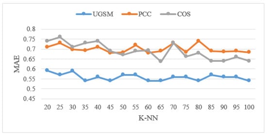
Figure 4.
MAE for different K-NN sizes of ML-20M using UGSM and other models. The x-axis is the K-NN size and the Y-axis is the MAE value.
It can be seen that the accuracy of the UGSM prediction was better when k = 5 and where MAE = 0.54. Therefore, in the rest of the experiments, the value of k was fixed to 35. For comparison, PCC scored the lowest, MAE = 0.68, when k = 60, and COS recorded MAE = 0.637 when k = 65. In the UGSM, “avr min sim” was derived using the following equation:
where represents the final NN for a; is the weight of average minimum similarity between a and ; i = 1, 2,…, and j = 1, 2…# of common g between a and .
In this model, we assumed that the weight of on kNN ()) had a significant role in enhancing the prediction accuracy by finding the proper neighbors. Therefore, we chose the optimal value for similarity according to the lowest MAE value and a suitable size of . The details are shown in Table 8.
Table 8.
MAE, NNf, and w min sim of adaptive ML-20M dataset.
From Table 8, it is notable that when k = 35, W.NNfa is distinct and higher than the rest of the neighbors recorded when k was greater or less than 35. W avr min sim was more significant than the remaining values, here w avr min sim = 0.5, with it, the minimum MAE was recorded. PCC and COS had an avr min sim = 0.2 and 0.23, respectively, with their ideal neighbor sizes. In comparison, the UGSM model picked up suitable neighbors with a smaller neighborhood size.
For the R2-yahoo music dataset, Figure 5 shows the results of the prediction accuracies of UGSM, PCC, and COS.
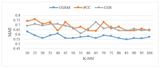
Figure 5.
MAE for different k sizes on R2-yahoo music dataset by UGSM and other models. The x-axis is the K-NN size and the Y-axis is the MAE value.
The accuracy of UGSM prediction is better when k = 45 and where MAE = 0.56. Therefore, in the rest of the experiments, the value of k was fixed to 45. PCC had the lowest MAE = 0.63 when k = 65; however, COS had a MAE = 0.61 when k = 55. Table 9 shows the values of avr min sim for the R2-yahoo music dataset.
Table 9.
MAE, NNf, and w min sim of adaptive R2-yahoo music dataset.
From Table 9, it can be seen that when k = 45, the W. NNf is high, and w avr min sim = 0.54. PCC and COS had an avr min sim = 0.18 and 0.21, respectively, and a greater MAE from their typical neighbor sizes. By comparing UGSM to the PCC and COS similarity measures in both datasets, the results demonstrated that UGSM captured better similarity, with a smaller neighborhood size and a small MAE. This result is a simple indication of UGSM’s ability to choose correct neighbors.
Experiment 2: Prediction Accuracy
This experiment contains three parts:
The first part assessed the UGSM method’s performance according to the predicted ratings’ accuracy by comparing it with PCC and COS. In the test stage, models produced a list of predicted ratings utilizing the test datasets. Then, we compared the predicted ratings to the original ratings in terms of MAE, predicted ratings’ level, and reliability between users. All results are shown in Figure 6.
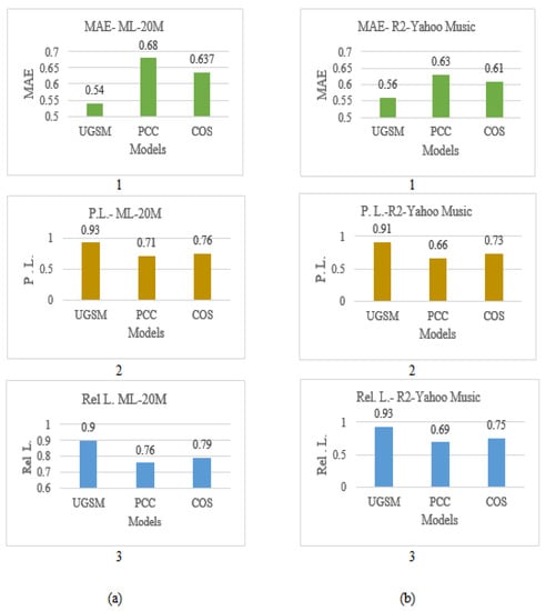
Figure 6.
Comparison of UGSM and traditional similarity measures according to (1) MAE; (2) P L; and (3) Rel L; for (a) ML-20M dataset and (b) R2-Yahoo Music dataset.
From the results in Figure 6, it is clear that the UGSM exceeds traditional similarity measures in both datasets since it produced an exceptional accuracy according to all tested evaluation metrics. When the k was the optimal value in all models, UGSM’s accuracy was significantly better than PCC and COS. Firstly, in Figure 6a (1) the results confirmed that UGSM decreased the MAE to 14.0% against PCC and 10.0% against COS for the ML-20M dataset. Secondly, Figure 6a (2) showed the P.L. of UGSM—22.0% and 17.0% better than PCC and COS, respectively. Finally, Figure 6a (3), by applying the Rel L metric, showed results and confirmed UGSM’s progress. It increased the Rel L between users by 14.0% and 11.0 % for PCC and COS. The same progress was obtained for the R2-yahoo music dataset.
In the second part, we compared the UGSM with modern CF algorithms in CF-SV according to Su et al. [36], the User-MRDC by Ai et al. [35], and the IOS by He et al. [52]. These studies used the ML1 dataset and MAE as the performance metric. Accordingly, we measured the MAE value for the same dataset using UGSM. We compared our findings to the results obtained in another study [36], where 3 to 150 neighbors were used. Table 10 shows the k neighbors tested in each algorithm, the number of neighbors, the k value at the Min MAE, and the best MAE value obtained by the indicated algorithms. Figure 7 shows the results.
Table 10.
Comparison of UGSM’s MAE to state-of-the-art algorithms.
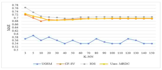
Figure 7.
Comparison of the UGSM’s accuracy to the state-of-the-art algorithms for the ML1 dataset. The X-axis is the K-NN and the Y-axis is the MAE value.
From Table 10, it is striking that UGSM gives the lowest MAE with a dynamic number of neighbors. From Figure 7, it is clear that the UGSM model has a better prediction accuracy than the compared algorithms in terms of all neighbor sizes. Since the UGSM does not directly depend on user ratings in selecting neighbors, its MAE is not affected much when changing the size.
In the third part, we compared UGSM to the proposed algorithm in [37], the UW algorithm, which has been compared to a variety of other approaches, including MSD, COS, Jaccard, PIP, and CJMSD [37]. It was applied in experiments to the ML-1M dataset. Thus, we used their dataset methodology with UGSM to compare them. Figure 8 demonstrates the MAE values for the ML-1M dataset for UGSM and several methods; k from 10 to 50, with increments of 5 per step.
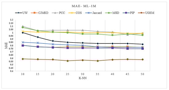
Figure 8.
MAE of the UGSM and the state-of-the-art studies for ML-1M dataset. The X-axis is the K-NN and the Y-axis is the MAE value. The results in Figure 8 show that the UGSM model outperforms the mentioned algorithms at all neighbor sizes. Unlike other methods, the UGSM is not affected much when increasing neighbor sizea, as it is almost stable with different neighbor sizes. When k = 50, most of the tested algorithms have improved accuracy. However, the UGSM accuracy is still the best; the prediction accuracy was improved by 24% against the UW method, 17% against the PIP method, and more than that against PCC and COS.
These results reflect the ability of UGSM to choose the appropriate neighbors for the active user, based on the global user’s taste for the item genre, thus increasing the power of the prediction model based on the local similarity among users.
5.4.2. Type 2: Experiment of Users with an Insufficient Number of Ratings
According to [21], the accuracy and quality of recommender systems decrease when entity information is insufficient. To check UGSM accuracy, we checked artificial users by establishing UGSM to handle only a few ratings from the datasets. Similar to the work in [42], we used a number of ratings, from 2 to 20. Then, we employed UGSM, PCC, and COS similarity measures to produce the predicted ratings; after that, we evaluated the results using MAE. Due to the long execution time, we randomly selected 100 users from each dataset to perform this experiment. Figure 9a,b shows the MAE for different methods outlined for a different number of ratings on ML-20M and R2-Yahoo music datasets, respectively.
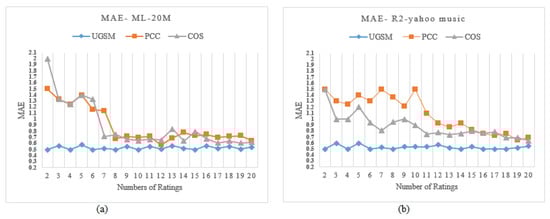
Figure 9.
MAE for (a) ML-20M dataset and (b) R2-Yahoo music dataset. The X-axis is the number of ratings and the Y-axis is the MAE value.
The results demonstrated that the UGSM behaves stably and produced better results than traditional similarity measures for all numbers of ratings for both datasets. Moreover, UGSM has notably better success than PCC and COS, even with very few available ratings, such as when the number of ratings = 2, 3, or 4.
6. Conclusions and Future Direction
In this study, a novel similarity measure has been suggested by exploiting the information of item genre to cover user preference similarities, even for users who having a very few available ratings. The study’s principal contribution is to produce user likenesses using preferred item genre information, as users generally like specific genres. Hence, two classes of user neighbors were determined to learn user relationships. The first class was the initial neighbor group, which contains user relationships according to every genre separately, who share their preferences with active users in a specific genre, based on average user preferences. The second class is the final neighbors group, which includes users who share their preferences in all genres with the active user.
Furthermore, we suggested two evaluation metrics to calculate the algorithm accuracy: the level of predicted ratings and the users’ reliability. We compared the UGSM to two traditional similarity measures: PCC and COS, in terms of MAE, level of predicted ratings, and user reliability to confirm UGSM performance. In addition, it was compared with modern collaborative filtering algorithms that introduced user similarity measures. Although the sparsity level was different in both tested datasets, UGSM performed stably and delivered better results than traditional similarity measures with smaller neighborhood sizes in regular user experiments and with users with few ratings.
Generally, in recommender systems, a similarity measure is used among users with a sufficient number of ratings; and another action is used between users who did not cast an adequate number of ratings. However, in this paper, the proposed model (UGSM) delivered accurate results for both user types at the same time.
Future studies plan to integrate the item genre into the item-based collaborative filtering algorithm to improve the item similarity measure and solve the cold-start problem. Besides, examining how user characteristics can improve the accuracy of a user-based CF algorithm.
Author Contributions
Conceptualization, J.A.-S. and C.K.; methodology, J.A.-S.; software, J.A.-S.; validation, J.A.-S.; formal analysis, J.A.-S. and C.K.; investigation, J.A.-S.; data curation, J.A.-S.; writing—original draft preparation, J.A.-S.; writing—review and editing, J.A.-S. and C.K. All authors have read and agreed to the published version of the manuscript.
Funding
This research received no external funding.
Institutional Review Board Statement
Not applicable.
Informed Consent Statement
Not applicable.
Data Availability Statement
Not applicable.
Conflicts of Interest
The authors declare no conflict of interest.
References
- Linden, G.; Smith, B.; York, J. Amazon.com recommendations: Item-to-item collaborative filtering. IEEE Internet Comput. 2003, 7, 76–80. [Google Scholar] [CrossRef] [Green Version]
- Bobadilla, J.; Ortega, F.; Hernando, A.; Gutiérrez, A. Recommender systems survey. Knowl. Based Syst. 2013, 46, 109–132. [Google Scholar] [CrossRef]
- Breese, J.S.; Heckerman, D.; Kadie, C. Empirical Analysis of Predictive Algorithms for Collaborative Filtering. In Proceedings of the Fourteenth Conference on Uncertainty in Artificial Intelligence (UAI-98), Madison, WI, USA, 24–26 July 1998; Cooper, G.F., Moral, S., Eds.; pp. 43–52. Available online: http://arxiv.org/abs/1301.7363 (accessed on 20 April 2021).
- Candillier, L.; Frank, M.; Fessant, F. Designing Specific Weighted Similarity Measures to Improve Collaborative Filtering Systems. In Proceedings of the Industrial Conference on Data Mining (ICDM): Advances in Data Mining. Medical Applications, E-Commerce, Marketing, and Theoretical Aspects, Leipzig, Germany, 16–18 July 2008; Volume 5077, pp. 242–255. [Google Scholar] [CrossRef]
- Bell, R.; Koren, Y.; Volinsky, C. The BellKor 2008 Solution to the Netflix Prize. Netflix Prize Documentation. Stat. Res. Dep. AT&T Res. 2009, 38 (Suppl. 1), 1–21. Available online: http://www.ncbi.nlm.nih.gov/pubmed/19898912 (accessed on 3 February 2021).
- Liu, H.; Hu, Z.; Mian, A.; Tian, H.; Zhu, X. A new user similarity model to improve the accuracy of collaborative filtering. Knowl. Based Syst. 2014, 56, 156–166. [Google Scholar] [CrossRef] [Green Version]
- Koren, Y.; Bell, R.; Volinsky, C. Matrix Factorization Techniques for Recommender Systems. Computer 2009, 30–37. [Google Scholar] [CrossRef]
- Sarwar, B.; Karypis, G.; Konstan, J.; Riedl, J. Item-based collaborative filtering recommendation algorithms. In Proceedings of the 10th International Conference on World Wide Web, WWW, Hong Kong, China, 1–5 May 2001; pp. 285–295. [Google Scholar] [CrossRef] [Green Version]
- Choi, S.M.; Ko, S.K.; Han, Y.S. A movie recommendation algorithm based on genre correlations. Expert Syst. Appl. 2012, 39, 8079–8085. [Google Scholar] [CrossRef]
- Santos, E.B.; Goularte, R.; Manzato, M.G. Personalized collaborative filtering: A neighborhood model based on contextual constraints. In Proceedings of the ACM Symposium on Applied Computing, Gyeongju, Korea, 24–28 March 2014; pp. 919–924. [Google Scholar] [CrossRef]
- Soares, M.; Viana, P. Tuning metadata for better movie content-based recommendation systems. Multimed. Tools Appl. 2015, 74, 7015–7036. [Google Scholar] [CrossRef]
- Li, Q.; Kim, B.M. Clustering approach for hybrid recommender system. In Proceedings of the IEEE/WIC International Conference on Web Intelligence (WI 2003), Halifax, NS, Canada, 13–17 October 2003; pp. 33–38. [Google Scholar] [CrossRef]
- Kim, K.R.; Moon, N. Recommender system design using movie genre similarity and preferred genres in SmartPhone. Multimed. Tools Appl. 2012, 61, 87–104. [Google Scholar] [CrossRef]
- Xue, G.R.; Lin, C.; Yang, Q.; Xi, W.; Zeng, H.J.; Yu, Y.; Chen, Z. Scalable collaborative filtering using cluster-based smoothing, SIGIR 2005. In Proceedings of the 28th Annual International ACM SIGIR Conference on Research and Development in Information Retrieval, Salvador, Brazil, 15–19 August 2005; pp. 114–121. [Google Scholar] [CrossRef]
- Ahn, H.J. Utilizing popularity characteristics for product recommendation. Int. J. Electron. Commer. 2006, 11, 59–80. [Google Scholar] [CrossRef]
- Subramaniyaswamy, V.; Logesh, R. Adaptive KNN based Recommender System through Mining of User Preferences. Wirel. Pers. Commun. 2017, 97, 2229–2247. [Google Scholar] [CrossRef]
- Middleton, S.E.; Alani, H.; de Roure, D.C. Exploiting Synergy Between Ontologies and Recommender Systems. Semant. Web Workshop 2002, 55, 41–50. [Google Scholar]
- Rashid, A.M.; Albert, I.; Cosley, D.; Lam, S.K.; McNee, S.M.; Konstan, J.A.; Riedl, J. Getting to know you: Learning new user preferences in recommender systems. In Proceedings of the 7th International Conference on Intelligent User Interfaces, San Francisco, CA, USA, 13–16 January 2002; pp. 127–134. [Google Scholar]
- Ren, L.; He, L.; Gu, J.; Xia, W.; Wu, F. A hybrid recommender approach based on Widrow-Hoff learning. In Proceedings of the 2008 2nd International Conference on Future Generation Communication and Networking, Hainan, China, 13–15 December 2008; Volume 1, pp. 40–45. [Google Scholar] [CrossRef]
- Al-Shamri, M.Y.H.; Bharadwaj, K.K. Fuzzy-genetic approach to recommender systems based on a novel hybrid user model. Expert Syst. Appl. 2008, 35, 1386–1399. [Google Scholar] [CrossRef]
- Ahn, H.J. A new similarity measure for collaborative filtering to alleviate the new user cold-starting problem. Inf. Sci. 2008, 178, 37–51. [Google Scholar] [CrossRef]
- Li, C.; Fang, W.; Yang, Y.; Zhang, X. Exploring Social Network Information for Solving Cold Start in Product Recommendation. In Proceedings of the International Conference on Web Information Systems Engineering, Miami, FL, USA, 1–3 November 2015. [Google Scholar] [CrossRef]
- Kim, H.N.; Ji, A.T.; Ha, I.; Jo, G.S. Collaborative filtering based on collaborative tagging for enhancing the quality of recommendation. Electron. Commer. Res. Appl. 2010, 9, 73–83. [Google Scholar] [CrossRef]
- Liu, C.Y.; Zhou, C.; Wu, J.; Hu, Y.; Guo, L. Social recommendation with an essential preference space. In Proceedings of the 32nd AAAI Conference on Artificial Intelligence, New Orleans, LA, USA, 2–7 February 2018; pp. 346–353. [Google Scholar]
- Zare, H.; Pour, N.; Mina, A.; Moradi, P. Enhanced recommender system using predictive network approach. Phys. A Stat. Mech. Appl. 2019, 520, 322–337. [Google Scholar] [CrossRef]
- Harper, F.M.; Konstan, J.A. The movielens datasets: History and context. ACM Trans. Interact. Intell. Syst. 2015, 5, 1–20. [Google Scholar] [CrossRef]
- Qian, X.; Feng, H.; Zhao, G.; Mei, T. Personalized recommendation combining user interest and social circle. IEEE Trans. Knowl. Data Eng. 2014, 26, 1763–1777. [Google Scholar] [CrossRef]
- Zhang, Y.; Song, W. A collaborative filtering recommendation algorithm based on item genre and rating similarity. In Proceedings of the 2009 International Conference on Computational Intelligence and Natural Computing, Wuhan, China, 6–7 June 2009; pp. 72–75. [Google Scholar] [CrossRef]
- Adomavicius, G.; Bamshad, M.; Ricci, F.; Tuzhilin, A. Context-aware recommender systems. In Recommender Systems Handbook, 2nd ed.; Springer: Boston, MA, USA, 2015; pp. 217–253. [Google Scholar] [CrossRef]
- O’Donovan, J.; Smyth, B.; Gretarsson, B.; Bostandjiev, S.; Höllerer, T. PeerChooser: Visual interactive recommendation. In Proceedings of the SIGCHI Conference on Human Factors in Computing Systems, Florence, Italy, 5–10 April 2008; pp. 1085–1088. [Google Scholar] [CrossRef]
- O’donovan, J.; Gretarsson, B.; Bostandjiev, S.; Höllerer, T.; Smyth, B. A visual interface for social information filtering. In Proceedings of the 12th IEEE 2009 International Conference on Computational Science and Engineering, Vancouver, BC, Canada, 29–31 August 2009; Volume 4, pp. 74–81. [Google Scholar] [CrossRef] [Green Version]
- Bostandjiev, S.; O’Donovan, J.; Höllerer, T. Tasteweights: A visual interactive hybrid recommender system. In Proceedings of the RecSys’12: Proceedings of the 6th ACM Conference on Recommender Systems, Dublin, Ireland, 9–13 September 2012; pp. 35–42. [Google Scholar] [CrossRef]
- Moscato, V.; Picariello, A.; Sperli, G. An emotional recommender system for music. IEEE Intell. Syst. 2020, 10, 1–10. [Google Scholar] [CrossRef]
- Frémal, S.; Lecron, F. Weighting strategies for a recommender system using item clustering based on genres. Expert Syst. Appl. 2017, 77, 105–113. [Google Scholar] [CrossRef]
- Ai, J.; Liu, Y.; Su, Z.; Zhang, H.; Zhao, F. Link Prediction in Recommender Systems based on Fuzzy Edge Weight Community Detection. EPL Europhys. Lett. 2019, 126. [Google Scholar] [CrossRef]
- Su, Z.; Zheng, X.; Ai, J.; Shen, Y.; Zhang, X. Link prediction in recommender systems based on vector similarity. Phys. A Stat. Mech. Appl. 2020, 560, 125154. [Google Scholar] [CrossRef]
- Chen, L.; Yuan, Y.; Yang, J.; Zahir, A. Improving the prediction quality in memory-based collaborative filtering using categorical features. Electronics 2021, 10, 214. [Google Scholar] [CrossRef]
- Yuan, Y.; Zahir, A.; Yang, J. Modeling implicit trust in matrix factorization-based collaborative filtering. Appl. Sci. 2019, 9, 4378. [Google Scholar] [CrossRef] [Green Version]
- Li, J.; Xu, W.; Wan, W.; Sun, J. Movie recommendation based on bridging movie feature and user interest. J. Comput. Sci. 2018, 26, 128–134. [Google Scholar] [CrossRef]
- Gogna, A.; Majumdar, A. A comprehensive recommender system model: Improving accuracy for both warm and cold start users. IEEE Access 2015, 3, 2803–2813. [Google Scholar] [CrossRef]
- You, T.; Rosli, A.N.; Ha, I.; Jo, G.-S. Clustering Method based on Genre Interest for Cold-Start Problem in Movie Recommendation. J. Intell. Inf. Syst. 2013, 19, 57–77. [Google Scholar] [CrossRef]
- Bobadilla, J.; Ortega, F.; Hernando, A.; Bernal, J. A collaborative filtering approach to mitigate the new user cold start problem. Knowl. Based Syst. 2012, 26, 225–238. [Google Scholar] [CrossRef] [Green Version]
- Yang, Z.; Wu, B.; Zheng, K.; Wang, X.; Lei, L. A survey of collaborative filtering-based recommender systems for mobile internet applications. IEEE Access 2016, 4, 3273–3287. [Google Scholar] [CrossRef]
- Asanov, D. Algorithms and Methods in Recommender Systems; Institute of Technology: Berlin, Germany, 2011. [Google Scholar] [CrossRef]
- Shardanand, U.; Maes, P. Social Information Filtering: Algorithms for Automating “Word of Mouth”. In Proceedings of the SIGCHI Conference on Human Factors in Computing Systems, Denver, CO, USA, 7–11 May 1995; pp. 1–15. [Google Scholar]
- Resnick, P.; Iacovou, N.; Suchak, M.; Bergstrom, P.; Riedl, J. GroupLens: An open architecture for collaborative filtering of netnews. In Proceedings of the 1994 ACM Conference on Computer Supported Cooperative Work, Chapel Hill, NC, USA, 22–26 October 1994; pp. 175–186. [Google Scholar] [CrossRef]
- Herlocker, J.; Konstan, J.A.; Riedl, J. An empirical analysis of design choices in neighborhood-based collaborative filtering algorithms. Inf. Retr. 2002, 5, 287–310. [Google Scholar] [CrossRef]
- Al-safi, J.K.S.; Kaleli, C. A Correlation and Slope Based Neighbor Selection Model for Recommender Systems. In Lecture Notes in Networks and Systems; Springer: Berlin/Heidelberg, Germany, 2021. [Google Scholar]
- Beel, J.; Genzmehr, M.; Langer, S.; Nürnberger, A.; Gipp, B. A comparative analysis of offline and online evaluations and discussion of research paper recommender system evaluation. In Proceedings of the International Workshop on Reproducibility and Replication in Recommender Systems Evaluation, Hong Kong, China, 12 October 2013; pp. 7–14. [Google Scholar] [CrossRef] [Green Version]
- Veras De Sena Rosa, R.E.; Guimaraes, F.A.S.; Mendonca, R.d.; de Lucena, V.F. Improving Prediction Accuracy in Neighborhood-Based Collaborative Filtering by Using Local Similarity. IEEE Access 2020, 8, 142795–142809. [Google Scholar] [CrossRef]
- Willmott, C.J.; Matsuura, K. Advantages of the mean absolute error (MAE) over the root mean square error (RMSE) in assessing average model performance. Clim. Res. 2005, 30, 79–82. [Google Scholar] [CrossRef]
- He, X.S.; Zhou, M.Y.; Zhuo, Z.; Fu, Z.Q.; Liu, J.G. Predicting online ratings based on the opinion spreading process. Phys. A Stat. Mech. Appl. 2015, 436, 658–664. [Google Scholar] [CrossRef]
Publisher’s Note: MDPI stays neutral with regard to jurisdictional claims in published maps and institutional affiliations. |
© 2021 by the authors. Licensee MDPI, Basel, Switzerland. This article is an open access article distributed under the terms and conditions of the Creative Commons Attribution (CC BY) license (https://creativecommons.org/licenses/by/4.0/).