Abstract
The importance of electricity in people’s daily lives has made it an indispensable commodity in society. In electricity market, the price of electricity is the most important factor for each of those involved in it, therefore, the prediction of the electricity price has been an essential and very important task for all the agents involved in the purchase and sale of this good. The main problem within the electricity market is that prediction is an arduous and difficult task, due to the large number of factors involved, the non-linearity, non-seasonality and volatility of the price over time. Data Science methods have proven to be a great tool to capture these difficulties and to be able to give a reliable prediction using only price data, i.e., taking the problem from an univariate point of view in order to help market agents. In this work, we have made a comparison among known models in the literature, focusing on Deep Learning architectures by making an extensive tuning of parameters using data from the Spanish electricity market. Three different time periods have been used in order to carry out an extensive comparison among them. The results obtained have shown, on the one hand, that Deep Learning models are quite effective in predicting the price of electricity and, on the other hand, that the different time periods and their particular characteristics directly influence the final results of the models.
MSC:
[2010] 00-01; 99-00
1. Introduction
Electricity is of great importance to society and essential for economic and industrial development. It is, in fact, one of the most important indicators for measuring the level of technological and industrial development of a country. It is a vital commodity and no day could be conceived without it. One of the biggest difficulties when talking about electricity management is that there is no way to store large quantities of it and, consequently, a constant balance between demand and supply is necessary, heading to highly volatile market prices [1].
In the 1990s, the electricity market underwent a process of deregulation [2], which meant that the market forces and the operator that manages the market were the ones that determined the balance between supply and demand and not the monopolistic system carried out by governments.
In the last decades of the 20th century, most electrical systems were reorganised, shifting from a vertically integrated structure of companies (in many cases national companies) to a structure of separate businesses (unbundling) [3]. The theoretical basis for this regulatory change was that, due to technological progress, economies of scale had disappeared in some of the links of the electricity system, so that the introduction of competition would lead to a greater welfare for society. Thus, while the transmission and distribution businesses still had strong natural monopoly characteristics (and therefore made sense to regulate them), competition was introduced for the generation and retail businesses. The generators, for their part, comprise the market supply, while the retailers aggregate energy demands, which they then deliver to end users [4].
Electricity price forecasting (EPF) has become a very valuable mechanism for all market partners in deregulated and competitive electricity markets, when this whole process is over, the system operator is responsible for setting a final price established for each hour of the current day.
In deregulated and competitive electricity markets, electricity price forecasting has become a high-priced tool for all market participants. Both producers and consumers use day-ahead price forecasts to determine their own bidding strategies to the electricity market. Consequently, the use of enhanced electricity price predictions strongly increases the revenues and decreases the risks of producers [5] and in the case of consumers, it maximizes their utilities [6] and may help with the identification of their needs [7]. Generally accurate forecasting results in lower scheduling costs because it can correctly predict the number of high-priced hours to avoid and the number of low-priced hours to be used [8].
Due to the proximity and the peculiarities of the Spanish electrical system, it was decided to choose this market as a case study, even though it is not one of the easiest to study due to its idiosyncrasy. Transparency measures taken by many governments have made possible free access to many of the data that were previously only accessible to those involved in this market. Nowadays any interested user can manage all the information available. The Spanish electricity market is managed by the Iberian Electricity Market (MIBEL) which was formed as a result of the integration in 2007 of the Spanish electricity system with the Portuguese system. The transmission network is operated by Red Eléctrica de España (REE) in Spain and Redes Energéticas Nacionais (REN) in Portugal, who manage and guarantee the operation. Regarding the management of the wholesale spot market, the authority responsible is the Iberian Energy Market Operator-Spanish Pole (OMIE). The Transmission System Operator (TSO) is Red Eléctrica de España (REE) and is responsible for ensuring the overall functioning and stability of the Spanish electricity system through the operation of the electricity system and the transmission of electricity. In order to achieve all these objectives and also to bring transparency to the system, REE has created an information system called the System Operator Information System (e-sios) which makes the results of the markets or system operation processes public [9]. Additionally, all the market information is provided by de OMIE too. (http://www.omie.es, accessed on 20 November 2020).
Many methods and ideas have been tried for electricity price forecasting, with varying degrees of success in Spain. In [10], a short-medium-term forecasting methodology based on calendar and temperature correction was proposed to forecast demand values in order to reveal its importance on the electricity price. Furthermore, in [11], an Auto-Regressive Integrated Moving Average (ARIMA) in combination with Radial Basis Function Neural Networks (RBFN) was proposed for electricity price data for the Spanish region with very good results. In this study, our main objective is to use Deep Learning techniques to be able to make an effective prediction of electricity prices in different significant periods of time in Spain. The proposed techniques have been Long short-term memory Networks (LSTM), Convolutional Neural Networks (CNN) and Temporal Convolutional Networks (TCN). In addition, we have used methods also known in the literature to serve as baseline and comparative to our proposal. Our contribution is founded on the application of novel techniques to the electricity market, as well as the search for the best parameters. The study of these architectures, as well as their parameterization will help us to achieve the best result, and also to be able to observe if there is a great difference in the effectiveness of the prediction according to the period being studied. Our study will be based on the conclusions obtained in the last review made so far by [12] where an exhaustive comparison on Deep Learning architectures for time series forecasting was made.
The rest of this paper is organized as follows: Section 2 introduces the Related Works. In Section 3, our methodology is defined in detail (data model, forecasting models, the experimental setup and the evaluation procedure). Section 4 explains all the experimental results obtained. Finally, Conclusions are provided in Section 5.
2. Related Works
Many methods and ideas for Electricity Price Forecasting (EPF) have been tried, with varying success. According to [13], EPF can be categorized in six major group models which could be reduced to five due to the fact that two groups can be combined into one larger class. The five groups are Statistical models, Reduced-form approaches, Fundamental methods, Multi-agent models and Computational Intelligence models.
Although a rather exhaustive classification has been made, it has been possible to verify throughout the work carried out with this subject, that generally, the methodologies used are a combination of some categories of this classification (hybrid methodologies), as can be seen in Figure 1. This tendency is due to the volatility of the electricity market, which makes any prediction in this field a challenge that can be seen from many different perspectives, even combining them.
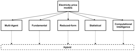
Figure 1.
Taxonomy of electricity price modelling approaches. The main model types could be combined as hybrid models.
Multi-agent models simulate the interplays between the agents and produce the price process by matching the demand and supply in the market. In 2014, in the work proposed by [14], they calculated suppliers’ optimal strategies in electricity markets with the use of competitive co-evolutionary algorithms. In [15], they use the Nash-Cournout framework to establish the correlations between wind power and electricity prices. In this type of framework, the market equilibrium is determined by the capacity setting decisions of the suppliers. Although this type of models are very flexible regarding the analysis of electricity market strategies and may seem an advantage a priori, in reality, it is a weakness since any decision must be previously modelled and justified. Usually, this type of model focuses more on qualitative rather than quantitative results, which is not very useful when it comes to predicting prices with great precision.
Fundamental methods model the impacts of physical and economic factors to describe the price dynamics. A fundamental model for the Nordic market was developed by [16]. In their proposal they considered 27 scalar parameters and 29 formulas to define the relationships between the fundamental variables and the price formula.
In 2013, using a stochastic model of the bid stack, the electricity prices were translated using the demand for power and the prices of generating fuels in [17].
Despite the good results obtained with this type of models, there are open challenges in the implementation of fundamental models, for example, data availability. Fundamental variables are often collected over longer time intervals, so these models are more suitable for medium-term predictions than short-term ones.
Reduced-form approaches describe the statistical properties of electricity price changes over time with the ultimate goal of derivative product evaluation and risk management; they do not provide accurate hourly price forecasts. One of the first publications on modelling electricity prices can be found in [18], where a Merton’s jump-diffusion model [19] was used. The problem with this type of models is that the performance obtained in forecasting the next day’s hourly price is not effective.
Statistical models use power market implementations of econometric models in order to forecast the electricity price. In the last years, there have been several proposals related to statistical models in EPF, in [20] a linear regression model in combination with regularization techniques was used. The main drawback of this type of methods is that the forecasting accuracy not only depends on the efficiency of the algorithms employed but also on the quality of the data analyzed, for example, in the presence of spikes, statistical models perform poorly.
Lastly, Computational Intelligence models combine learning, evolution and ambiguity to create methods that can adjust to complicated dynamic systems. Artificial neural networks, fuzzy systems, support vector machines and evolutionary computation are the principal algorithms of Computational Intelligence models. The main advantage of these methods is their flexibility and the capacity to handle complex and non-linear data. Due to the increase in computing capacity available today, this type of model is the most widely used, because, although its greatest weakness is the time cost involved, the efficiency in terms of accuracy is high. In [21], a combination of two deep neural networks was proposed for an electricity price forecasting system. Furthermore, in the work proposed by [22], an artificial neural network (ANN) in combination with clustering algorithms was used for day-ahead price forecasting. Huan et al. presented in [7] the SEPNet method consisting of a combination of three algorithms (Variational Mode Decomposition, Convolutional Neural Network and Gated Recurrent Unit) to predict the price of electricity using data from New York City over the period 2015 to 2018. Lastly, in [23], a novel methodology is proposed to Electricity Price Forecasting in Australia. This method carried out a Tensor Canonical Correlation Analysis (TCC) to remove redundant factors, then a Deep Neural Network (DNN) with a novel Stacked Pruning Sparse Denoising Autoencoder (SPSDAE) is used to decrease the noise of datasets, and finally a new multi-modal combined (MMC) method is used to predict the day-ahead cost of electricity.
Given the rise of the methods included in this last category, there has been a great increase in their use in problems related to the prediction of electricity prices. Due to the temporal features that this type of problem has, it is usually seen from the perspective of time series forecasting, as in [24], where recurrent neural networks were used or in [25], where a hybrid model of adam optimized LSTM neural network was proposed.
Table 1 provides a summary of the papers, divided into categories, mentioned in this section.

Table 1.
Related work on electricity market price forecasting within each of the categories (established by [13]) into which the different models published in the literature so far fall.
3. Methodology
In this section, we present the models used in the forecasting methodology and the experimental setup.
3.1. Time Series Forecasting Models
According to the review carried out in [12], where many different architectures were compared, LSTM, CNN, and TCN were the ones which obtained the best results. In order to test the performance of these models against other models, we have decided to use three other well-known models in the literature, on the one hand another but simpler Deep Learning model namely Multilayer Perceptron (MLP), and on the other hand Machine Learning models, such as Regression Trees and Random Forest.
3.1.1. Long Short-Term Memory Network
Long Short-Term Memory (LSTM) networks were introduced in 1997 [26]. They can model temporal dependencies in larger horizons without forgetting the short-term patterns.
LSTM networks are composed of units that are called LSTM memory cells [26], these cells contain some gates that process the inputs. These gates are:
- Input gate, which takes care of preventing the memory cell from being modified by irrelevant perturbations.
- Output gate, which takes care of protect other cells from perturbations stored in the current memory cell.
- Forget gate, which allows the memory cell to reset the information if it becomes irrelevant.
3.1.2. Convolutional Neural Networks
Convolutional Neural Networks (CNN) architectures have been a dominant method in computer vision tasks since the astonishing results were shared on the object recognition competition known as the ImageNet Large Scale Visual Recognition Competition (ILSVRC) in 2012 [27]. Nowadays, they are the state of the art of many classification tasks like object recognition, speech recognition, and natural language processing.
CNN architecture can extract features from high dimensional raw data with a grid topology without any feature engineering. This can be made with the convolutional method, a sliding filter that creates a features map and captures the repeated patterns at different input regions. Furthermore, the convolutional method provides to this architecture a characteristic called “distortion invariance”, which involves that features are extracted no matter where they are in the data.
The architecture of CNN is composed of convolution layers, pooling layers, and fully connected layers. Furthermore, CNN architecture is based on the principles of:
- Local connectivity because each node is connected only to a region of the input.
- Shared weights because all neurons in the same layers share the same weight matrix for the convolution.
- Translation equivariance.
These properties allow CNNs to have a smaller number of trainable parameters than RNNs. For these reasons, CNNs are most efficient in the training time. Another essential aspect of CNNs is the ability to stack different convolutional layers so that the deep learning model can be more high-performance and obtain a better representation of the time series at different scales.
3.1.3. Temporal Convolutional Network
Temporal Convolutional Network (TCN) is a new architecture of CNN but more specialized in temporal series. This architecture is inspired by Wavenet autoregressive model [28], which was designed for audio generation problems.
TCN architecture is an adapted CNN with these special characteristics:
- Convolutions are causal to prevent information loss.
- The architecture can process a sequence of any length and map into an output of the same length.
TCN architecture uses dilated causal convolutions to learn the long-term dependencies in the time series. These convolutions increase the network’s receptive field without losing resolution because the pooling operation is not needed. Additionally, residual connections are employed to increase the network’s depth to deal effectively with an extensive history size.
TCN has low memory requirements for training due to shared convolutional filters, long input sequences can be processed with parallel convolutions, and are more stable training schemes.
3.1.4. Multilayer Perceptron
Multilayer Perceptron (MLP) is the most basic type of feed-forward artificial neural network. This neural network is composed by three main type of layers: input, hidden and output. The architecture is variable but in general will consist in one input layer, several hidden layers and an output layer [29].
The number of hidden layers will determine the depth of the network. It is the inclusion of more hidden layers which makes a MLP network a deep learning model. Each of the layers is in turn composed of neurons connected by parameters that are modified in the learning process of the algorithm. The objective of this learning is to map and find the relationship between the expected input and output.
3.1.5. Regression Tree
Decision trees are characterized as machine learning models that are quite easy to interpret and have a fairly high accuracy. Regression trees are a special type of decision trees that deal with a continuous goal variable, as electricity price [30].
Regression trees are built through an iterative process that splits each node into child nodes using some rules. This process ends with the construction of a model or a tree-like graph. Each of the nodes of the tree is fitted to get the predicted values of the output variables when new samples are used.
3.1.6. Random Forest
Random Forests (RF) build a large number of regression trees in order to solve regression tasks. These trees, which act as regression functions, are combined using bootstrap or ensemble techniques in order to come to a final decision. When RF is used for regression problems, the output variables are fitted by using samples of the input variables. For each input variable, divide the data into several points, and calculate the sum of squared errors (SSE) for the predicted value and the actual value at each divided point. Then, choose the minimum SSE value for this node. In addition, the importance of variables can be obtained by permuting the values of all input variables and measuring their prediction accuracy differences in out-of-bag samples [31].
3.2. Experimental Setup
The methodology of our work has been divided in two well-differentiated parts as can be seen in Figure 2. The first step is to find the best hyperparameters for each model (Train/Test Step). Once these parameters, and therefore the best model, have been found, the model is trained on a time period different from the previous one (Validation Step), in order to validate it reliably and avoid over-fitting. In both phases, a Multi-Input Multi-Output (MIMO) technique has been used.
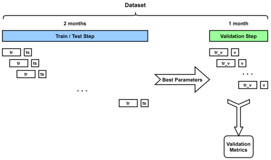
Figure 2.
Scheme followed in our proposal using the MIMO strategy. To improve the reliability of the results, the dataset is divided in two subsets: The first subset will be used to train and search for the best hyperparameters of the model, the input-output pairs are formed by training and testing sample time points named and . The second subset will be used to validate the model on a new dataset once the best hyperparameters are identified, in order to avoid overfitting. In this case the input-output pairs are formed by and v.
The first stage is to obtain the data to be used, which consists of a univariate time series (only one variable) that will serve as input to the models to be compared. This time series is formed by the electricity price of the period of time to be studied, which can be obtained from the e-sios website.
As in [12], we have used the Multi-Input Multi-Output (MIMO) technique to train and evaluate the models. The MIMO strategy increases the predictions’ accuracy since it does not accumulate previous predictions’ errors. This strategy makes use of a sliding window scheme to create the input-output pairs that will be used by the models to be tested. All these output pairs have a fixed prediction window, in this case 24 h, while the training window has a size defined by a factor whose value also has to be optimized [32]. In both phases, we have tried to make the prediction of day as realistic as possible, i.e., at a set time on day D, the market price values are predicted for each hour of day .
To test our models, we have divided our originals datasets in two subsets: train dataset and validation dataset. The training dataset is used to train and search the best parameters of the models, and once they are found, we evaluate their accuracy with the validation dataset. The training datasets include all data except the last month of each dataset, which will be found in the validation datasets.
To evaluate each model, we obtain the model’s prediction feeding it with the validation dataset windows. For any window of the validation dataset, the model will predict the next window. Therefore, we can connect all the predicted windows and compare the forecasted time series’s accuracy with the original one. The input-output pairs for this phase are and v, respectively.
However, before we can obtain the predictions of each model, they must have been trained before. To train the models, they must be fed previously with the training subsets (tr and tr_v, respectively), which follow the same moving window philosophy as validation subsets (ts and v).
3.2.1. Hyperparameter Optimization Step
We have based the experimental setup of this paper on [12], in which they have adjusted the parameters for each model used in the article. The parameters to be optimized are those that better identify each model, taking into account the characteristics of each one.
These parameters have been collected in a grid, where they try to use different values for any model and parameters. The grid parameters are determined based on the typical values in the literature of each model. In all cases, many hyperparameters must be configured. To establish a fair comparison among architectures, they have explored from a single layer to a deeper network on every occasion. Since there are many parameters that have been considered, we have decided to refer only to those that are most important for each model. However, all the parameters used as well as their possible values can be found in the repository located at [33].
As mentioned above, our datasets have been divided into two parts, one for training and one for validation. The search for hyperparameters has been carried out with this first subdivision (training part), for which the sliding window strategy has been followed, so that each of the models has an input layer with as many neurons as the “past history” parameter indicates (tr) and an output layer with as many neurons as the prediction horizon has been established , in this case 24 h (ts).
First, we explore the LSTM architecture, which has three main parameters and can generate 18 different models. These parameters are the number of recursive layers stacked, the number of recursive units in each layer, and whether the last layer returns the order of states or just the final state. If the return sequence is False, the last layer returns a value for each cycle unit. If the return sequence is True, the last layer returns a value for each time step, forming a shape matrix ( × ). Similarly, as we are in a multi-step-ahead forecasting problem, the LSTM model’s output is connected to a dense layer with one neuron for prediction. The number of layers in the LSTM model ranges from 1 to 4, and the number of units varies from 32 to 168. An overview of the parameters used can be seen in Table 2.
Table 2.
Grid of parameters used for LSTM models.
As far as CNN models are concerned, they are composed of stacked convolution blocks, constituting a one-dimensional convolution along layer followed by a max-pooling layer. The convolutional blocks use decreasing kernel size, as it is usual in the literature. Single-layer models have a kernel of size 3, two-layers models have kernel sizes of 5 and 3, and four-layers models have kernels of size 7-5-3, and 3.We have only considered a pooling factor of 2, as the input sequence in the datasets is not excessively long. All the parameters used are summed up in Table 3.
Table 3.
Grid of parameters used for CNN models.
TCN models are defined by five principally parameters: number of layers, number of convolutional filters, dilation factors, convolutional kernel size, and whether to return the final output or the full sequence. The number of dilations and the kernel sizes have been selected according to the receptive field of the TCN, which follows the formula ( × × ). All the parameters used can be seen in the table below (Table 4).
Table 4.
Grid of parameters used for TCN models.
Multilayer Perceptrons are characterized as simple neural networks for which the main difficulty is to find the best combination between the number of layers and neurons, as well as the filters. The following table shows the configuration of hidden layers used in this work. All the parameters used can be seen in Table 5.
Table 5.
Grid of parameters used for MLP models.
Decision trees are defined by four main parameters, these are, splitter, max depth, min samples split and min samples leaf. Splitter defines the strategy used to choose the split at each node, the two supported strategies are “best” to choose the best split and “random” to choose the best random split. Max depth parameter establish the maximum depth of the tree. Min samples split is the minimum number of samples requires to split an internal node. Lastly, min samples leaf is the minimum number of samples required to be at a leaf node. All the parameters used can be seen in Table 6.
Table 6.
Grid of parameters used for regression tree models.
Lastly, a Random Forest can be defined by four main parameters as well, number of estimators, max depth, min samples split and min samples leaf. The last three parameters mean the same as in decision trees, the only different parameter is the number of estimators which represents the number of the trees in the forest. All the parameters used can be seen in Table 7.
Table 7.
Grid of parameters used for random forest models.
3.2.2. Validation Step
Once the best hyperparameters have been obtained in the first step, the validation of the model is carried out. This consists of predicting each day of the validation subset, also using the sliding window strategy. To make this possible, the model is fed with information from the previous days (tr_v), defined by the “past history” factor, and the next day is predicted. Once the predictions have been obtained (o), they are compared to the actual price (v) to obtain the real effectiveness of each of the models.
Concerning to metrics, the predictions are evaluated with MAE, WAPE, MASE and MAPE functions. All of these functions provide different information about the accuracy of the forecasted time series.
Mean absolute error (MAE) is similar to MSE (Mean squared error), but instead of applying a square, it applies an absolute value. MAE uses the same scale as the data being measured and it is a standard measure to forecast error in time series analysis [34].
Weighted average percentage error (WAPE) [35] is the most different metric of the chosen ones. WAPE is a variation of MAPE, where the error is rescaled dividing it by the mean. Due to this, the error is comparable across time series of varying scales. Thanks to these properties, scale-independency and interpretability, WAPE is widely used to measure the forecast accuracy, and it is very recommended for forecasting with intermittent and low-volume data.
Mean absolute scaled error (MASE) is similar to MAE, but it has some properties that makes it a recommended metric to compare forecast accuracy. An example is the property of symmetry, which penalises positive and negative errors equally, as it does with the long and shorts forecast errors.
Mean absolute percentage error (MAPE) is calculated by averaging the absolute error divided by the observed values. This approach is useful when the size of a prediction variable is significant in evaluating the accuracy of a prediction [36].
Finally, and given that time is also a variable to be taken into account when talking about Deep Learning and Machine Learning models, it has been decided to add the average time (T) taken to train each of the models as a validation metric.
4. Results
In this section, we describe the experiments that were carried out to analyze the performance of the proposal. Firstly, selected datasets are described. Secondly, a comparison of the results obtained by the models explained in the previous section is included. Lastly, the software and hardware infrastructure used is specified.
4.1. Datasets Description
In Spain, the electricity system underwent a process of liberalisation between 1997 and 1998 [37], in which the tasks of transmission and distribution (regulated) and generation and retail (competitive) were separated as it has been presented above. The Spanish electricity market is in charge of the OMIE, and it is organised in sequential sessions: the day-ahead, intraday, and balancing sessions.
The price of electricity is different for each of the hours of each day; this price is established by means of an auction. First, power generation companies and wholesale retailers buyers are convened in the day-ahead spot market to send their quotes that include energy price pairs within 24 h of the next day. The market operator (MO) is responsible for clearing the market and providing a temporary energy plan for each bidder within 24 h of the next day. By matching all the purchase and sale bids, the electricity market establishes the price that the energy will have for each of the hours of the following day, i.e., the hourly marginal price is obtained at the intersection of the supply and demand curves [38].
Every day, between 12:30 and 13:00 of the current day D, the price that the energy will have in each of the hours of the following day , within the daily market, is made public [39].
As it can be intuited, it is very important for the system operators to have an idea of what the prices may be in the short term, as this will significantly influence the offers they make, so a system capable of making predictions for the next day is an indispensable tool for them [40].
The main objective of this study is to see how the choice of data can influence the effectiveness of the prediction results. For each of the chosen data sets, three months have been selected, with a total of 2208 time points (hours) for each dataset, with two of them being used to set the parameters of the models (train/test step), and the remaining month to validate them (validation step).
For each of the three data sets, a normalization of the data has been carried out, the type of normalization is also a parameter to be chosen in the first stage, the possible values are a minmax or z-score normalization. Attempts have been made to choose time periods with some particularity. These are detailed below:
- Fraud Period: In 2019, the National Commission for Markets and Competition (CNMC) fined Endesa and Naturgy for altering electricity prices between October 2016 and January 2017 [41], the months chosen for this study. This period will help to test how sensitive the models are to periods that may present tax irregularities. To make the results more comparable, the following periods used will have the same length, i.e., three months. Hourly electricity price in this period can be observed in Figure 3 where the yellow line represents the mean price of all the period.
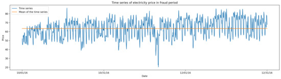 Figure 3. Time series of fraud period. On the x-axis we can see that this period covers electricity prices between October 2016 and January 2017, when the Fraud was reported. The horizontal line observed indicates the average for that period which is 63.46, a much higher value than the other periods in the study.
 - Normal period: In order to have a reference period, a stage has been chosen in which no anomalies were detected, unlike the two next data sets. This stage covers the months from September to December 2019. Figure 4 represents the hourly electricity price in this period, with the mean represented by a horizontal yellow line.
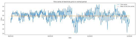 Figure 4. Time series of normal period. On the x-axis we can see that this period covers electricity prices from September to December 2019. The horizontal line which can be seen indicates the average for that period with a value of 48.91.
 - Quarantine Period: The year 2020 marked a change in many daily habits due to the global pandemic. One of the most notable changes was the increase in electricity consumption, as people spent more time at their homes due to quarantine requirements. The three months from 15 March 2020 to 15 June 2020 have been chosen to represent this stage. Hourly electricity price in this period can be observed in Figure 5 where the yellow line represents the mean price of all the period.
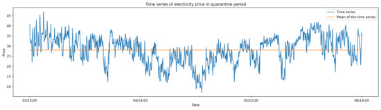 Figure 5. Time series of quarantine period. On the x-axis we can see that this period covers electricity prices between 15 March 2020 and 15 June 2020. The horizontal line shown indicates the average for this period, which is 28.09.
4.2. Experimental Results
This part of the study focuses on presenting the results obtained in terms of forecasting accuracy over the validation dataset for each dataset and each model used. The metrics used for this purpose were MAE, WAPE, MASE, MAPE and Time (T).
Table 8 shows a summary of the best parameter configuration obtained for each dataset and metric, specifying the best model for each one of them.
Table 8.
Best parameter settings obtained for each dataset and each metric. For each of the possible scenarios, there is a description of which specific algorithm has obtained the best results as well as the best hyperparameters.
Table 9 presents a comparison between the results obtained with the different architectures for each dataset in terms of MAE. For each of the datasets, the best result is specified in bold. In quarantine period, the best result was obtained with the LSTM model, with an average error of 3.535 €. Regarding normal period, the best model was CNN, with an average error of around 4.125 €. Finally, the lowest error for the fraud period was obtained with a regression tree, resulting in an average error of 4.034 €. The last row and column of the table represent the mean MAE for each model and dataset, respectively. The best average model is LSTM and the dataset with the lowest average MAE error is the quarantine period.
Table 9.
MAE results for each period and each model. The results have been obtained after choosing the best set of parameters for each case by carrying out a parameter optimization process. The last row and column correspond to the means for each model and dataset, respectively. The best model for each dataset is specified in bold.
Concerning WAPE, the results obtained can be seen in Table 10. In case of the quarantine period, the best model was LSTM with an average WAPE of 0.112. Secondly, for the normal period the best model was CNN with a percentage of 0.084. Finally, for fraud the best model was the regression tree with an average WAPE of 0.059. The last row and column of the table represent the average WAPE per model and dataset, respectively. As with MAPE, the best mean model is LSTM, while for the datasets, the best results are obtained with the fraud period.
Table 10.
WAPE results for each period and each model. The results have been obtained after choosing the best set of parameters for each case by carrying out a parameter optimization process. The last row and column correspond to the means for each model and dataset, respectively. The best model for each dataset is specified in bold.
The results in terms of MASE (Table 11) follow the same pattern as for the previous two metrics. The best result for the quarantine period is obtained with the LSTM model with a value of 2.600, for the normal period the best result is 1.764 using a CNN model. Finally, for the fraud period a best result of 1.458 is obtained with decision trees. In average terms, the lowest error is obtained with the fraud period, and in terms of model with an LSTM network, as was the case for WAPE and MAE.
Table 11.
MASE results for each period and each model. The results have been obtained after choosing the best set of parameters for each case by carrying out a parameter optimization process. The last row and column correspond to the means for each model and dataset, respectively. The best model for each dataset is specified in bold.
MAPE is the only metric that differs from the others as can be seen in Table 12. In this case, for the normal period, the best score is obtained with trees, with a value of 0.095, while for quarantine and fraud the best result is still LSTM and Trees, with 0.126 and 0.059, respectively, as was the case for the three previous metrics.
Table 12.
MAPE results for each period and each model. The results have been obtained after choosing the best set of parameters for each case by carrying out a parameter optimization process. The last row and column correspond to the means for each model and dataset, respectively. The best model for each dataset is specified in bold.
Considering the four tables together, it can be observed that the same patterns are repeated in most cases, i.e., for each period the best model coincides for MAE, WAPE, MASE and MAPE. If the average of these measures with respect to the datasets is taken into account, the influence of each of the datasets on the final result is clearly evidenced. The most characteristic case is the fraud period, which had on average a higher price than the other two periods, resulting in a higher average MAE. However, for the case of WAPE, the fraud period is the one that achieves a lower average WAPE, which is due to the fact that this metric is divided by the mean of the values, so the higher the mean, the lower the WAPE. Something similar happens with MASE and MAPE, as it can be observed that for the fraud period the values are lower with respect to the other two periods, this is due to the fact that they are metrics inversely proportional to the values of the time series.
Table 13 shows the average training time for each of the cases presented in this work. If we take into account the data sets, there is not much difference between the training, since the length of the time series is the same. In contrast, the average time taken for each model is significantly different from one model to the other, with the tree model being the fastest and the LSTM networks the slowest. The total time spent on training and validation can also be seen in Table 14
Table 13.
Time results in seconds for each period and each model. The results in time were obtained by calculating the average of each of the times used to train each of the models in the parameter optimisation process.
Table 14.
Total time in seconds for training and validation of each of the models.
Finally, Figure 6, Figure 7 and Figure 8 provide a graphical comparison between the predictions on the validation set and the actual price values. The graphs show the results obtained with the best model in terms of MAE for each of the three datasets.
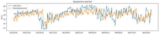
Figure 6.
Comparison between actual and predicted price by model LSTM using validation data for the quarantine data period.
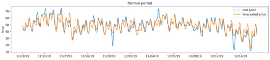
Figure 7.
Comparison between actual and predicted price by model CNN using validation data for the normal data period.
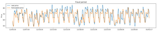
Figure 8.
Comparison between actual and predicted price by model Tree using validation data for the fraud data period.
Looking at all the metrics presented, both those that take into account the efficiency of predictions and time, we can observe a drawback that occurs in many works, which is that the models that take the longest time are the ones that obtain the best results. In this case, it can be clearly seen that on average the model that takes the longest is LSTM, while on average it is the one that obtains the best predictions. This is why it is sometimes necessary to choose between these two fundamental aspects, computation time and prediction efficiency. Regarding which technique should be used, we have to say that since it is a very complex problem, the choice of which technique is more appropriate will depend on the input data, however, it can be corroborated that regardless of the particular Deep Learning technique we use the results are promising.
4.3. Software and Experimental Setting
All the data used in this study have been collected thanks to the API provided by the System Operator Information System (e-sios). This API allows for data retrieval in JSON format through a code in Python so that it can be then processed.
Due to the large amount of experiments carried out, the executions were performed on an Intel machine, specifically Intel(R) Core(TM) i7-8700 CPU @ 3.20GHz, with 64 GB of RAM and 12 cores. The source code with the different tests performed in this study can be found in [33].
5. Conclusions
In this paper, we have made a comparison among different well-known models in architecture and their use in the prediction of electricity market prices. This comparison has been made by optimising the parameters for each of the algorithms and each of the datasets used. Given the temporal nature of the electricity price, we decided to study different time periods, specifically three, one of which served as a baseline (normal period), another period in which fraud was detected in the electricity market (fraud period) and finally the period that included the quarantine months in 2020, due to the pandemic (quarantine period).
The results obtained have shown that the electricity market is clearly influenced by the social and economic circumstances that are occurring on a particular day, which is why it is important to take into account the ideosyncrasy of the data and use models in accordance with this fact.
Of all the models used, three stand out: LSTM, CNN and Regression Trees. These three models are the ones that on average have given the best results for each of the validation metrics used, specifically, LSTM has obtained better results in the case of the quarantine period, CNN for the normal period and finally Trees for the fraud period.
In terms of execution time, Deep Learning models have taken the longest, while Machine Learning models have taken the shortest. This is probably the biggest limitation in our study, the big difference between the time of the hyperparameter search and the training and validation time itself. However, once the hyperparameter search has been performed, the time taken to train the model and validate it is negligible. Given this limitation we also propose to look at this problem from the Data Streaming point of view, so that the model only has to be trained once. One of the disadvantages of neural networks is precisely that, the execution time they consume, however, they have proven to be a very good choice if a high percentage of prediction success is the objective of the task.
In view of the results obtained, it can be said that for the specific case study we have dealt with, the Spanish electricity market, the results obtained with the different techniques are quite promising. As for which technique in particular is the best, we have to say that being such a complex problem there is no single technique that works well for all data sets, but what we can assure in view of the results is that Deep Learning techniques work well for this type of problem.
This paper has focused on a time series study from a univariate point of view, i.e., the price is predicted taking into account only the past of this variable. As future work we propose the use of exogenous variables that have a direct correlation with price, such as demand [42], renewable energy capacity, balancing market price or trade value as used in [43], thus moving from a univariate to a multivariate problem. Testing with all possible variables is an almost impossible task, but the future objective we propose is to collect information on a wide range of variables and use only those that have a high degree of correlation with the variable to be predicted. Furthermore, given the large use of these models in the literature, we believe that it would be interesting to make use of ensemble technologies to make the final prediction, as this paradigm allows the advantages of individual models to be combined to make a final model.
Author Contributions
Conceptualization, B.V.-M. and Á.A.-V.; methodology, B.V.-M.; software, B.V.-M.; validation, C.R.-E., I.A.N.-C. and Á.A.-V.; formal analysis, B.V.-M.; investigation, B.V.-M.; resources, C.R.-E. and I.A.N.-C.; data curation, Á.A.-V. and B.V.-M.; writing—original draft preparation, B.V.-M.; writing—review and editing, C.R.-E., I.A.N.-C. and Á.A.-V.; visualization, B.V.-M.; supervision, C.R.-E., I.A.N.-C. and Á.A.-V.; project administration, C.R.-E. and I.A.N.-C.; funding acquisition, C.R.-E. and I.A.N.-C. All authors have read and agreed to the published version of the manuscript.
Funding
This research has been funded by FEDER/Ministerio de Ciencia, Innovación y Universidades—Agencia Estatal de Investigación/Proyecto TIN2017-88209-C2 and by the Andalusian Regional Government under the projects: BIDASGRI: Big Data technologies for Smart Grids (US-1263341), Adaptive hybrid models to predict solar and wind renewable energy production (P18-RT-2778).
Institutional Review Board Statement
Not applicable.
Informed Consent Statement
Not applicable.
Data Availability Statement
The data presented in this study are available on https://github.com/bvegaus/electric (accessed on 29 April 2021).
Conflicts of Interest
The authors declare no conflict of interest.
References
- Ortiz, M.; Ukar, O.; Azevedo, F.; Múgica, A. Price forecasting and validation in the Spanish electricity market using forecasts as input data. Int. J. Electr. Power Energy Syst. 2016, 77, 123–127. [Google Scholar] [CrossRef]
- Weron, R. Electricity price forecasting: A review of the state-of-the-art with a look into the future. Int. J. Forecast. 2014, 30, 1030–1081. [Google Scholar] [CrossRef]
- Kahn, A.E. The Economics of Regulation: Principles and Institutions; MIT Press: Cambridge, MA, USA, 1988; Volume 1. [Google Scholar]
- Anbazhagan, S.; Kumarappan, N. Day-ahead deregulated electricity market price forecasting using recurrent neural network. IEEE Syst. J. 2012, 7, 866–872. [Google Scholar] [CrossRef]
- Maciejowska, K.; Nitka, W.; Weron, T. Enhancing load, wind and solar generation for day-ahead forecasting of electricity prices. Energy Econ. 2021, 99, 105273. [Google Scholar] [CrossRef]
- Yang, Z.; Ce, L.; Lian, L. Electricity price forecasting by a hybrid model, combining wavelet transform, ARMA and kernel-based extreme learning machine methods. Appl. Energy 2017, 190, 291–305. [Google Scholar] [CrossRef]
- Huang, C.J.; Shen, Y.; Chen, Y.H.; Chen, H.C. A novel hybrid deep neural network model for short-term electricity price forecasting. Int. J. Energy Res. 2021, 45, 2511–2532. [Google Scholar] [CrossRef]
- Mathaba, T.; Xia, X.; Zhang, J. Analysing the economic benefit of electricity price forecast in industrial load scheduling. Electr. Power Syst. Res. 2014, 116, 158–165. [Google Scholar] [CrossRef]
- Red Eléctrica de España, S.A.U.R. Esios: Sistema de Información del Operador del Sistema. 2020. Available online: https://www.esios.ree.es (accessed on 20 November 2020).
- Segarra-Tamarit, J.; Perez, E.; Belenguer, E.; Cardo-Miota, J.; Beltran, H. Aggregated demand analysis and forescasting methodology for the Iberian Electricity Market. In Proceedings of the 2020 2nd IEEE International Conference on Industrial Electronics for Sustainable Energy Systems (IESES), Cagliari, Italy, 1–3 September 2020; Volume 1, pp. 255–260. [Google Scholar]
- Shafie-Khah, M.; Moghaddam, M.P.; Sheikh-El-Eslami, M. Price forecasting of day-ahead electricity markets using a hybrid forecast method. Energy Convers. Manag. 2011, 52, 2165–2169. [Google Scholar] [CrossRef]
- Lara-Benıtez, P.; Carranza-Garcıa, M.; Riquelme, J.C. An Experimental Review on Deep Learning Architectures for Time Series Forecasting. arXiv 2021, arXiv:2103.12057. [Google Scholar]
- Weron, R. Modeling and Forecasting Electricity Loads and Prices: A Statistical Approach; John Wiley & Sons: Hoboken, NJ, USA, 2007; Volume 403. [Google Scholar]
- Ladjici, A.A.; Tiguercha, A.; Boudour, M. Nash Equilibrium in a two-settlement electricity market using competitive coevolutionary algorithms. Int. J. Electr. Power Energy Syst. 2014, 57, 148–155. [Google Scholar] [CrossRef]
- Rubin, O.D.; Babcock, B.A. The impact of expansion of wind power capacity and pricing methods on the efficiency of deregulated electricity markets. Energy 2013, 59, 676–688. [Google Scholar] [CrossRef]
- Vehviläinen, I.; Pyykkönen, T. Stochastic factor model for electricity spot price—The case of the Nordic market. Energy Econ. 2005, 27, 351–367. [Google Scholar] [CrossRef]
- Carmona, R.; Coulon, M.; Schwarz, D. Electricity price modeling and asset valuation: A multi-fuel structural approach. Math. Financ. Econ. 2013, 7, 167–202. [Google Scholar] [CrossRef][Green Version]
- Kaminski, V. The challenge of pricing and risk managing electricity derivatives. In The US Power Market-Restructuring and Risk Management; Elsevier BV: Amsterdam, The Netherlands, 1997. [Google Scholar]
- Matsuda, K. Introduction to Merton Jump Diffusion Model; The Graduate Center, Department of Economics, The City University of New York: New York, NY, USA, 2004. [Google Scholar]
- Tutun, S.; Bataineh, M.; Aladeemy, M.; Khasawneh, M. The Optimized Elastic Net Regression Model for Electricity Consumption Forecasting; San Francisco, CA, USA, 2016. [Google Scholar]
- Kuo, P.H.; Huang, C.J. An electricity price forecasting model by hybrid structured deep neural networks. Sustainability 2018, 10, 1280. [Google Scholar] [CrossRef]
- Panapakidis, I.P.; Dagoumas, A.S. Day-ahead electricity price forecasting via the application of artificial neural network based models. Appl. Energy 2016, 172, 132–151. [Google Scholar] [CrossRef]
- Sun, L.; Li, L.; Liu, B.; Saeedi, S. A Novel Day-ahead Electricity Price Forecasting Using multi-modal combined Integration via Stacked Pruning Sparse Denoising Auto Encoder. Energy Rep. 2021, 7, 2201–2213. [Google Scholar] [CrossRef]
- Ugurlu, U.; Oksuz, I.; Tas, O. Electricity price forecasting using recurrent neural networks. Energies 2018, 11, 1255. [Google Scholar] [CrossRef]
- Chang, Z.; Zhang, Y.; Chen, W. Electricity price prediction based on hybrid model of adam optimized LSTM neural network and wavelet transform. Energy 2019, 187, 115804. [Google Scholar] [CrossRef]
- Hochreiter, S.; Schmidhuber, J. Long short-term memory. Neural Comput. 1997, 9, 1735–1780. [Google Scholar] [CrossRef]
- Yamashita, R.; Nishio, M.; Do, R.K.G.; Togashi, K. Convolutional neural networks: An overview and application in radiology. Insights Imaging 2018, 9, 611–629. [Google Scholar] [CrossRef]
- Oord, A.v.d.; Dieleman, S.; Zen, H.; Simonyan, K.; Vinyals, O.; Graves, A.; Kalchbrenner, N.; Senior, A.; Kavukcuoglu, K. Wavenet: A generative model for raw audio. arXiv 2016, arXiv:1609.03499. [Google Scholar]
- Gardner, M.W.; Dorling, S. Artificial neural networks (the multilayer perceptron)—A review of applications in the atmospheric sciences. Atmos. Environ. 1998, 32, 2627–2636. [Google Scholar] [CrossRef]
- Torgo, L. Functional Models for Regression Tree Leaves; ICML; Morgan KAufman: Burlington, MA, USA, 1997; Volume 97, pp. 385–393. [Google Scholar]
- Zhang, J.; Ma, G.; Huang, Y.; Aslani, F.; Nener, B. Modelling uniaxial compressive strength of lightweight self-compacting concrete using random forest regression. Constr. Build. Mater. 2019, 210, 713–719. [Google Scholar] [CrossRef]
- Lara-Benítez, P.; Carranza-García, M.; Luna-Romera, J.M.; Riquelme, J.C. Temporal convolutional networks applied to energy-related time series forecasting. Appl. Sci. 2020, 10, 2322. [Google Scholar] [CrossRef]
- Vega, B.; Solís, J. Electricity Time Series Forecasting. 2020. Available online: https://github.com/bvegaus/electric (accessed on 11 February 2020).
- Hyndman, R.J.; Koehler, A.B. Another look at measures of forecast accuracy. Int. J. Forecast. 2006, 22, 679–688. [Google Scholar] [CrossRef]
- Kim, S.; Kim, H. A new metric of absolute percentage error for intermittent demand forecasts. Int. J. Forecast. 2016, 32, 669–679. [Google Scholar] [CrossRef]
- Khair, U.; Fahmi, H.; Al Hakim, S.; Rahim, R. Forecasting error calculation with mean absolute deviation and mean absolute percentage error. J. Phys. Conf. Ser. 2017, 930, 012002. [Google Scholar] [CrossRef]
- Jordana, J.; Levi-Faur, D.; Puig, I. The Limits of Europeanization: Regulatory Reforms in the Spanish and Portuguese Telecommunications and Electricity Sectors. Governance 2006, 19, 437–464. [Google Scholar] [CrossRef]
- Cruz, A.; Muñoz, A.; Zamora, J.L.; Espínola, R. The effect of wind generation and weekday on Spanish electricity spot price forecasting. Electr. Power Syst. Res. 2011, 81, 1924–1935. [Google Scholar] [CrossRef]
- Díaz, G.; Coto, J.; Gómez-Aleixandre, J. Prediction and explanation of the formation of the Spanish day-ahead electricity price through machine learning regression. Appl. Energy 2019, 239, 610–625. [Google Scholar] [CrossRef]
- Nogales, F.J.; Contreras, J.; Conejo, A.J.; Espínola, R. Forecasting next-day electricity prices by time series models. IEEE Trans. Power Syst. 2002, 17, 342–348. [Google Scholar] [CrossRef]
- País, E. La CNMC Multa a Endesa y Naturgy con 25 Millones por Alterar los Precios de la Electricidad. 2019. Available online: https://elpais.com/economia/2019/05/14/actualidad/1557846131_807016.html (accessed on 20 November 2020).
- Zhang, J.L.; Zhang, Y.J.; Li, D.Z.; Tan, Z.F.; Ji, J.F. Forecasting day-ahead electricity prices using a new integrated model. Int. J. Electr. Power Energy Syst. 2019, 105, 541–548. [Google Scholar] [CrossRef]
- Oksuz, I.; Ugurlu, U. Neural network based model comparison for intraday electricity price forecasting. Energies 2019, 12, 4557. [Google Scholar] [CrossRef]
Publisher’s Note: MDPI stays neutral with regard to jurisdictional claims in published maps and institutional affiliations. |
© 2021 by the authors. Licensee MDPI, Basel, Switzerland. This article is an open access article distributed under the terms and conditions of the Creative Commons Attribution (CC BY) license (https://creativecommons.org/licenses/by/4.0/).