
A Survey for Recent Techniques and Algorithms of Geolocation and Target Tracking in Wireless and Satellite Systems


Abstract
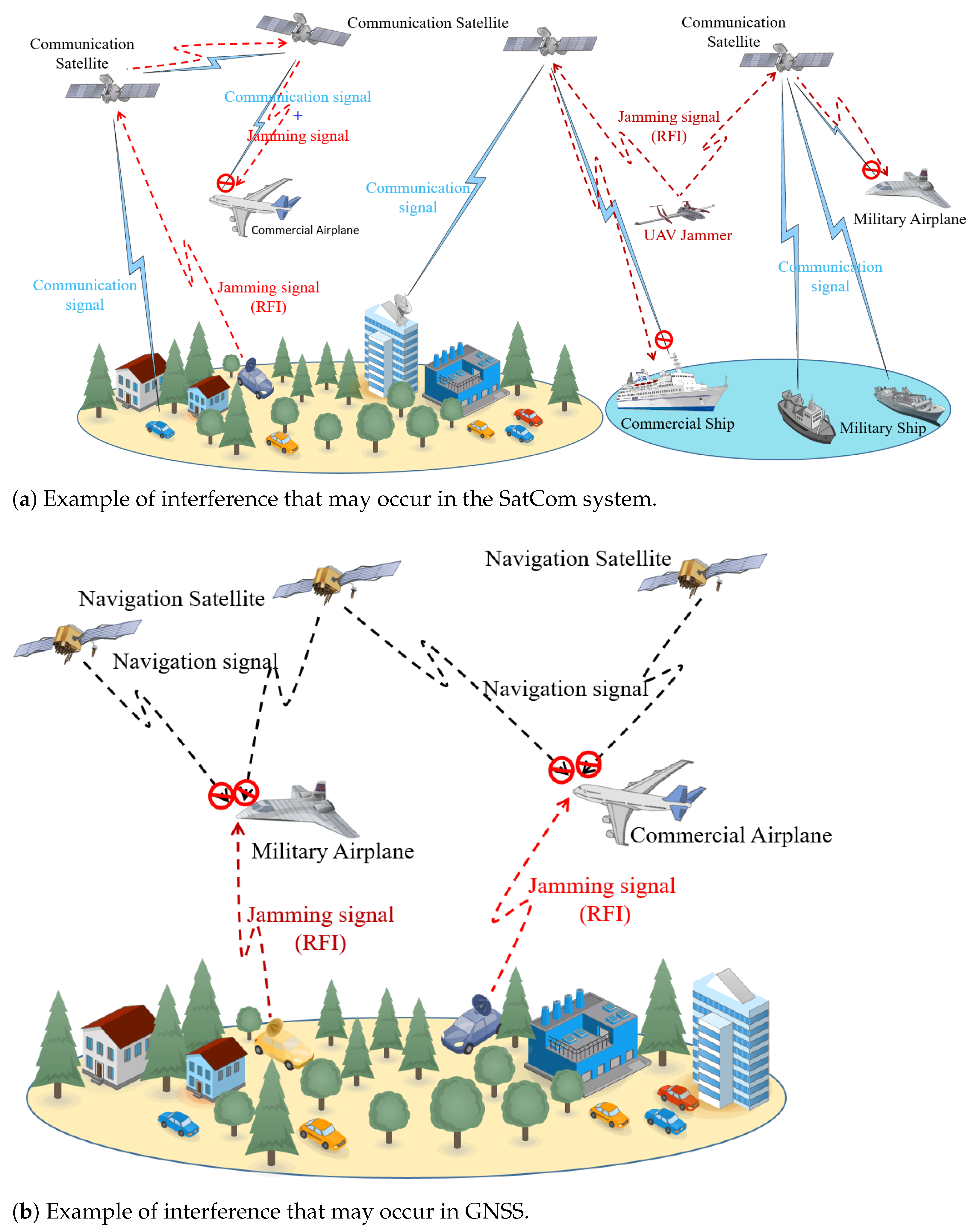
1. Introduction
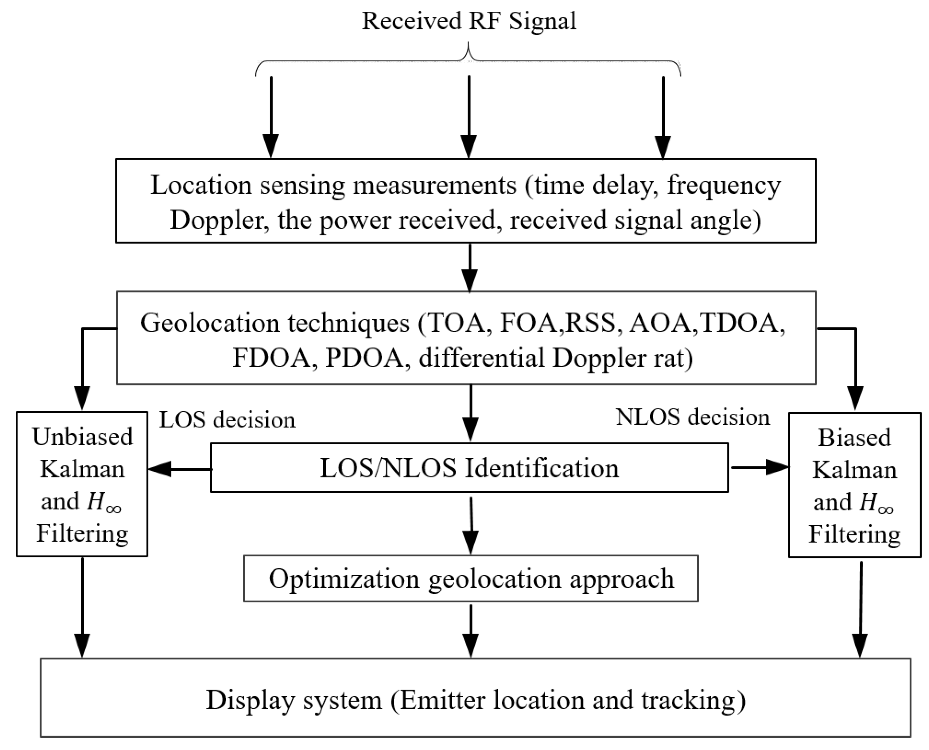
2. Geolocation and Target Tracking System
- The front end equipment for RF signal sensing.
- The geolocation equipment that allows the measurement and determination of the relative position of the RF emitter.
- The optimization approaches that allow optimization of geolocation and target tracking algorithms, as well as organizing the non-linear equations within a set of linear equations.
- The optimal state estimation tools, which allow the data smoothing filtering using Kalman filtering.
- The display system that allows a display of the position estimation and trajectory of the stationary or mobile RF emitter.
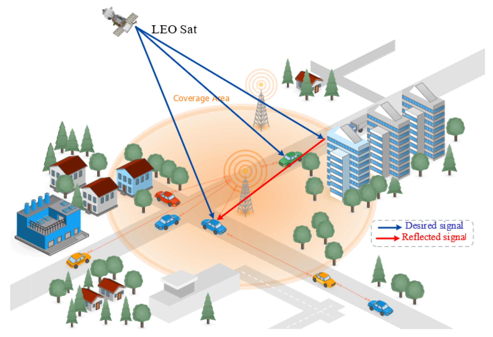
Urban Environment Characteristics
3. Conventional Geolocation Techniques
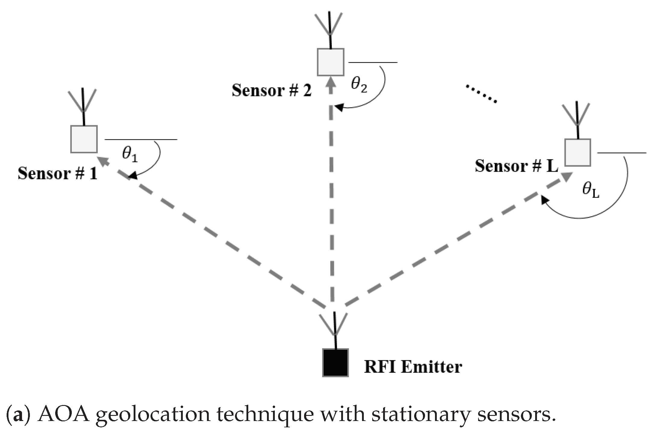
3.1. Angle of Arrival (AOA)
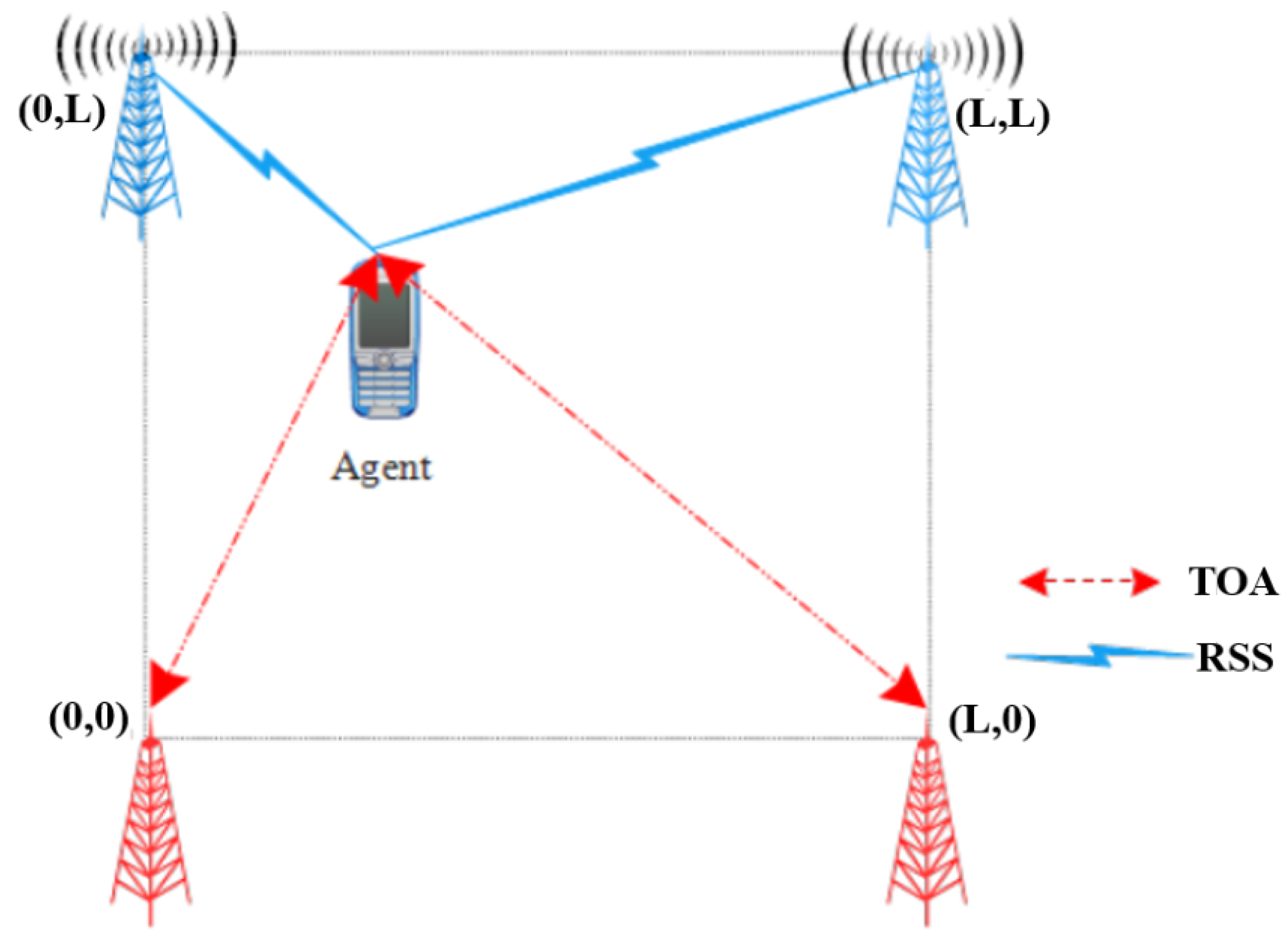
3.2. Time of Arrival (TOA)
3.3. Time Difference of Arrival (TDOA)
3.4. Received Signal Strength (RSS)
3.5. Power Difference of Arrival (PDOA)
3.6. Frequency Difference of Arrival (FDOA)
3.7. Hybrid Technique of Geolocation Measurements
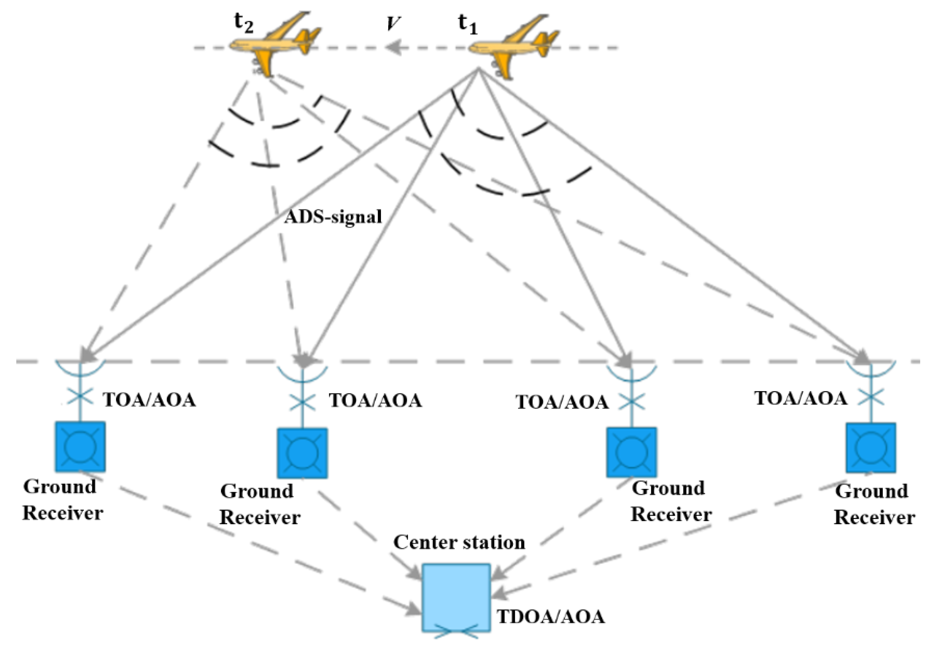
3.7.1. TDOA/AOA
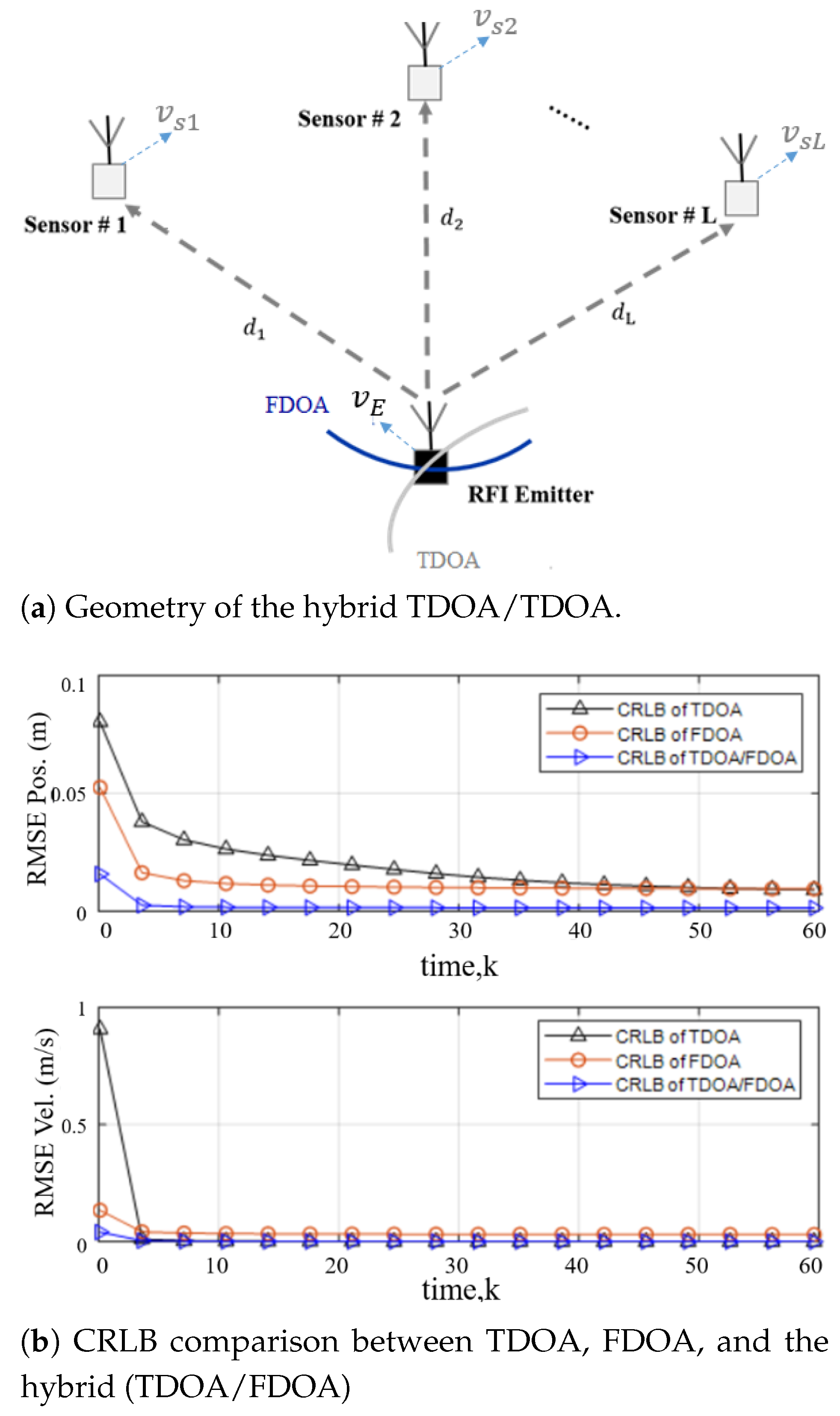
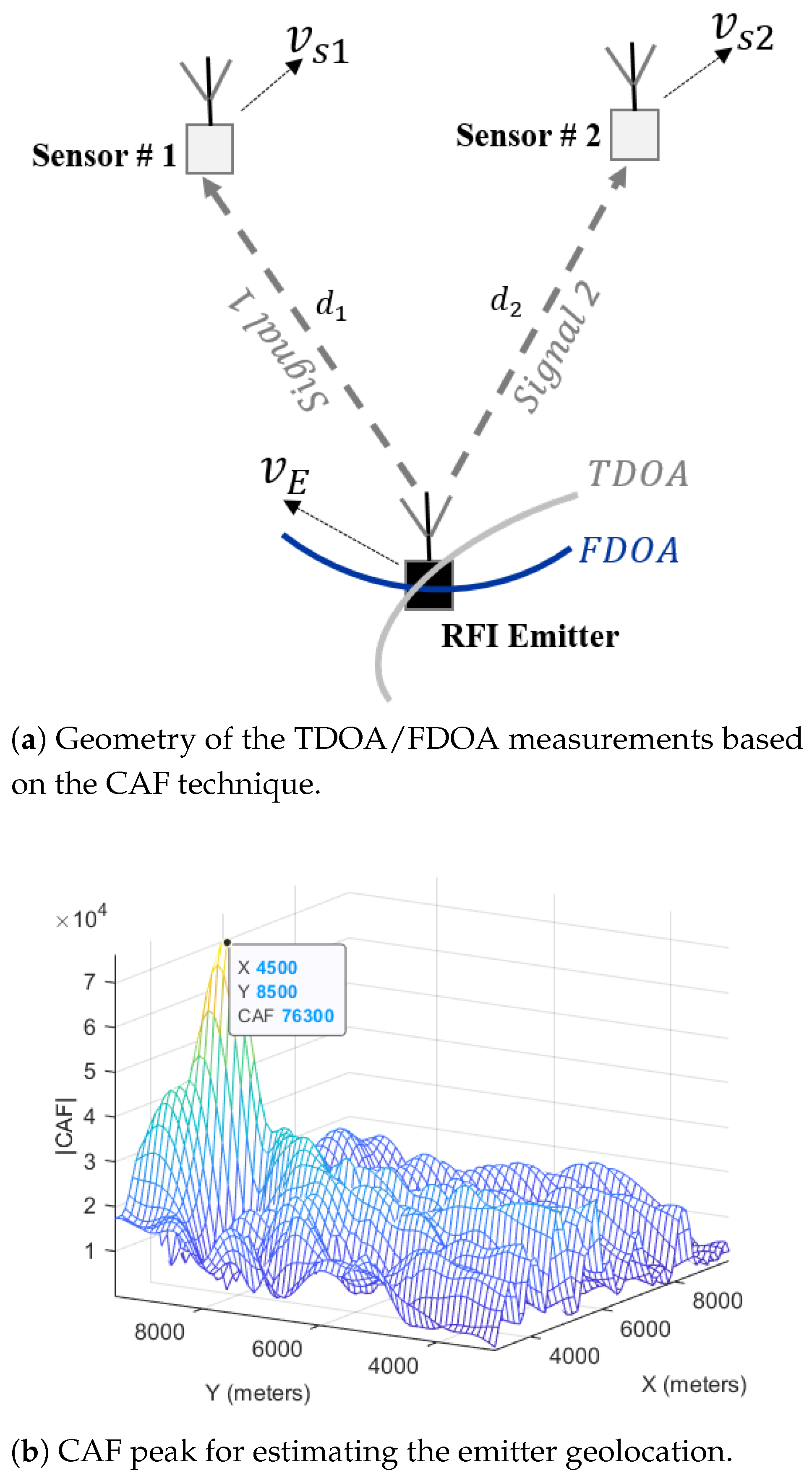
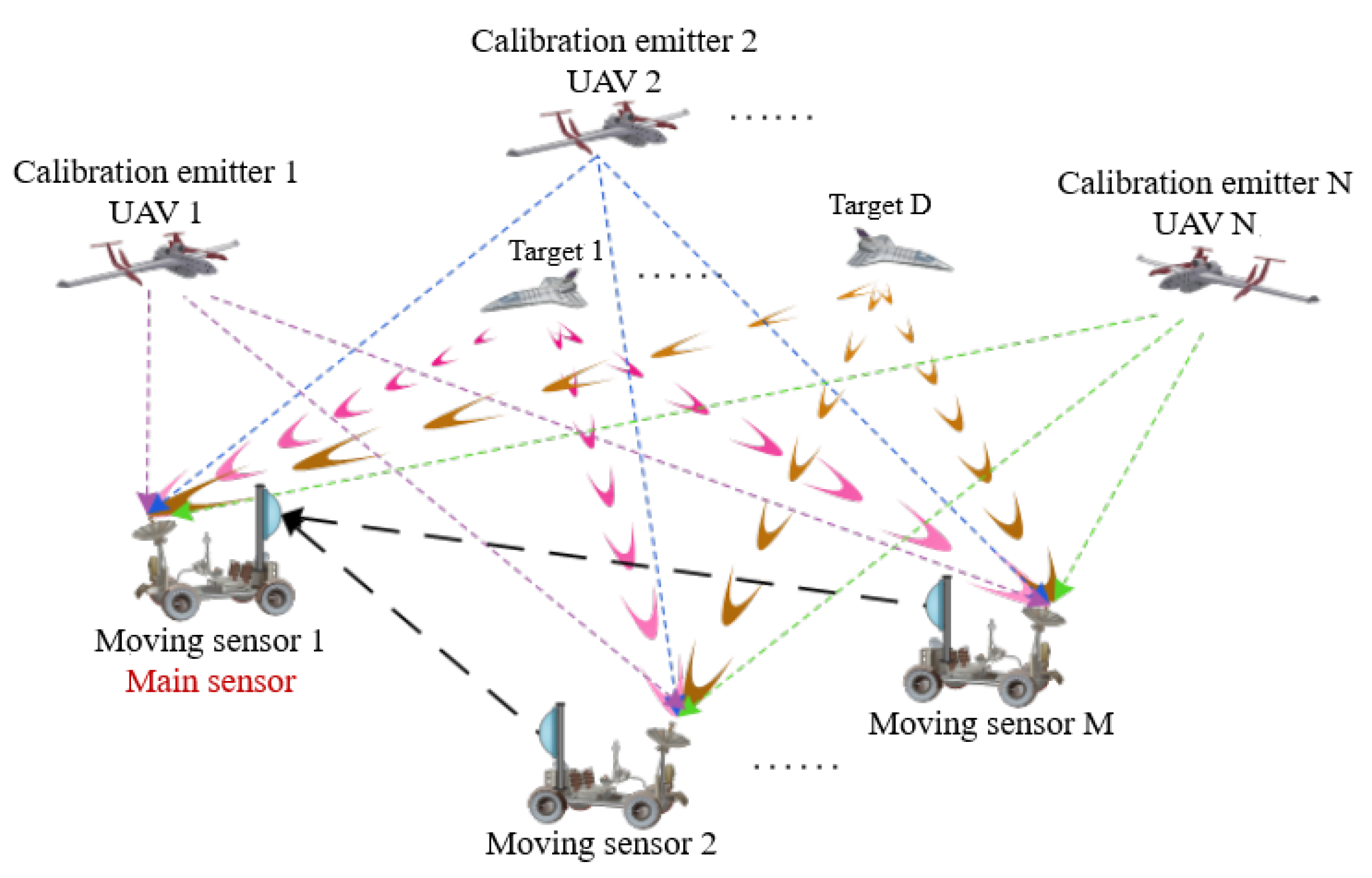
3.7.2. TDOA/FDOA
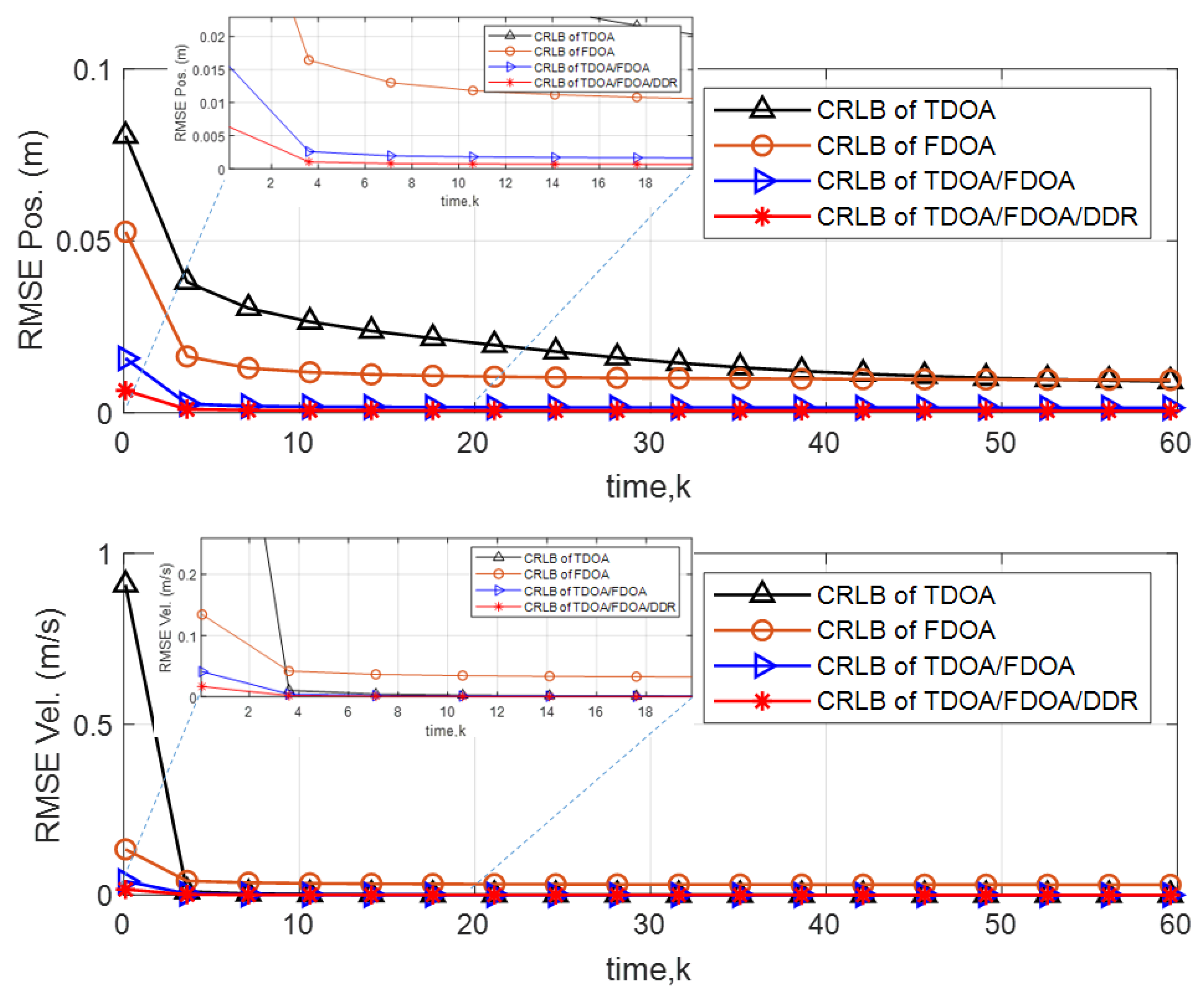
3.8. Tri-Combination Technique of Geolocation Measurements
4. Approaches of Optimizing Geolocation Measurements
4.1. Taylor Series (TS)
4.2. Maximum Likelihood Estimator (MLE)
4.3. Least Square (LS)
4.4. Weighted Least Square (WLS)
4.5. Artificial Intelligence (AI)
4.5.1. Genetic Algorithm (GA)
4.5.2. Dempster–Shafer (D-S)
4.5.3. Machine Learning (ML) and Deep Learning (DL) Approaches
5. Approaches of Optimal State Estimation Utilizing Filtering
5.1. Kalman Filter (KF)
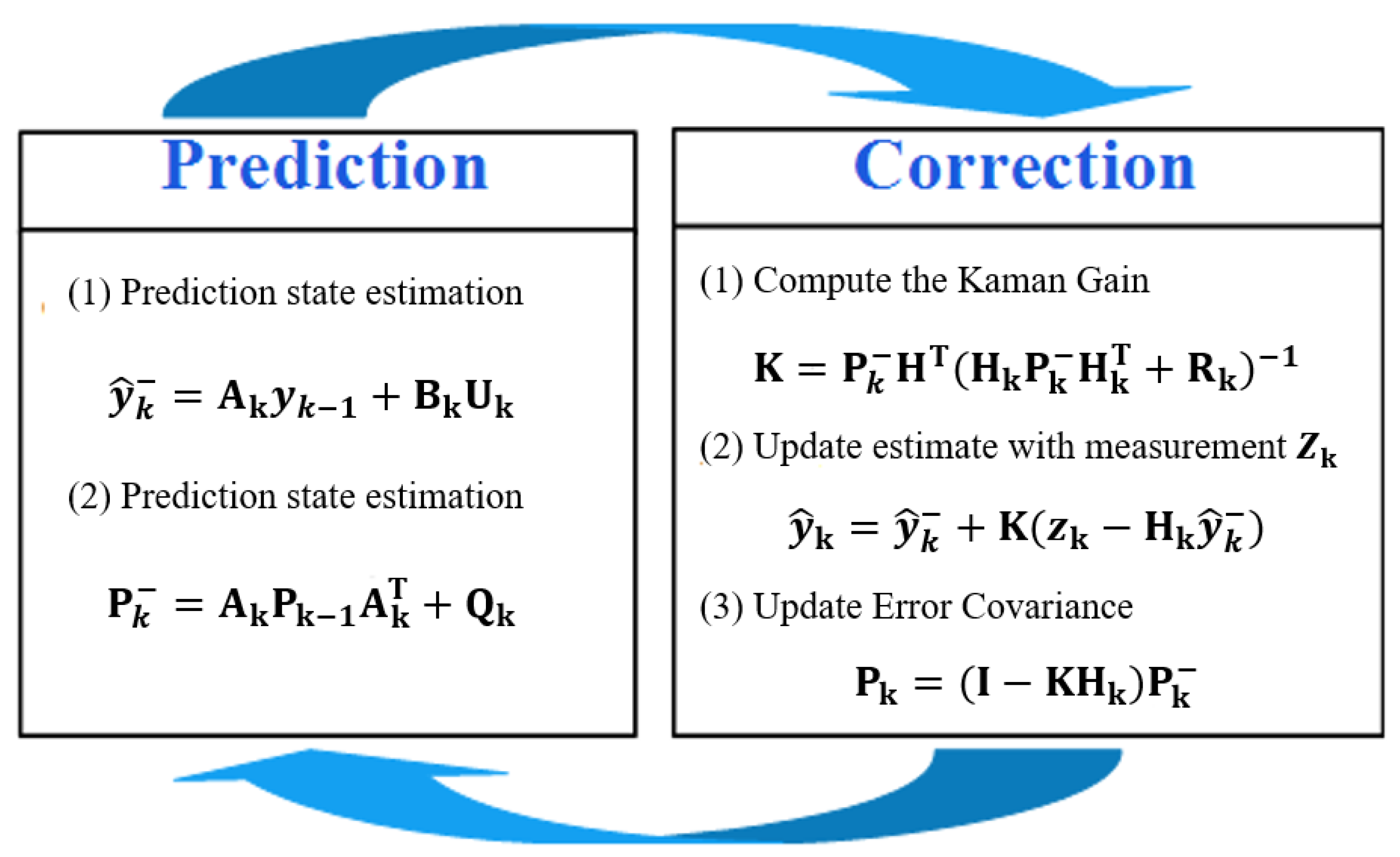
Kalman Filtering Algorithm
- (i)
- The time update equations are in charge of projecting the current state and error covariance estimates forward at a time in order to obtain a priori estimates for the next time stage.
- (ii)
- The feedback—that is, integrating a new measurement into the a priori estimate to produce an improved a posteriori estimate—is handled by the measurement update equations. Time update equations are also known as predictor equations, while measurement update equations are known as corrector equations. Indeed, as shown in Figure 19, the final estimation algorithm resembles a predictor-corrector algorithm for solving numerical problems [107].
5.2. Extended Kalman Filter (EKF)
5.3. Adaptive Extended Kalman Filter (AEKF)
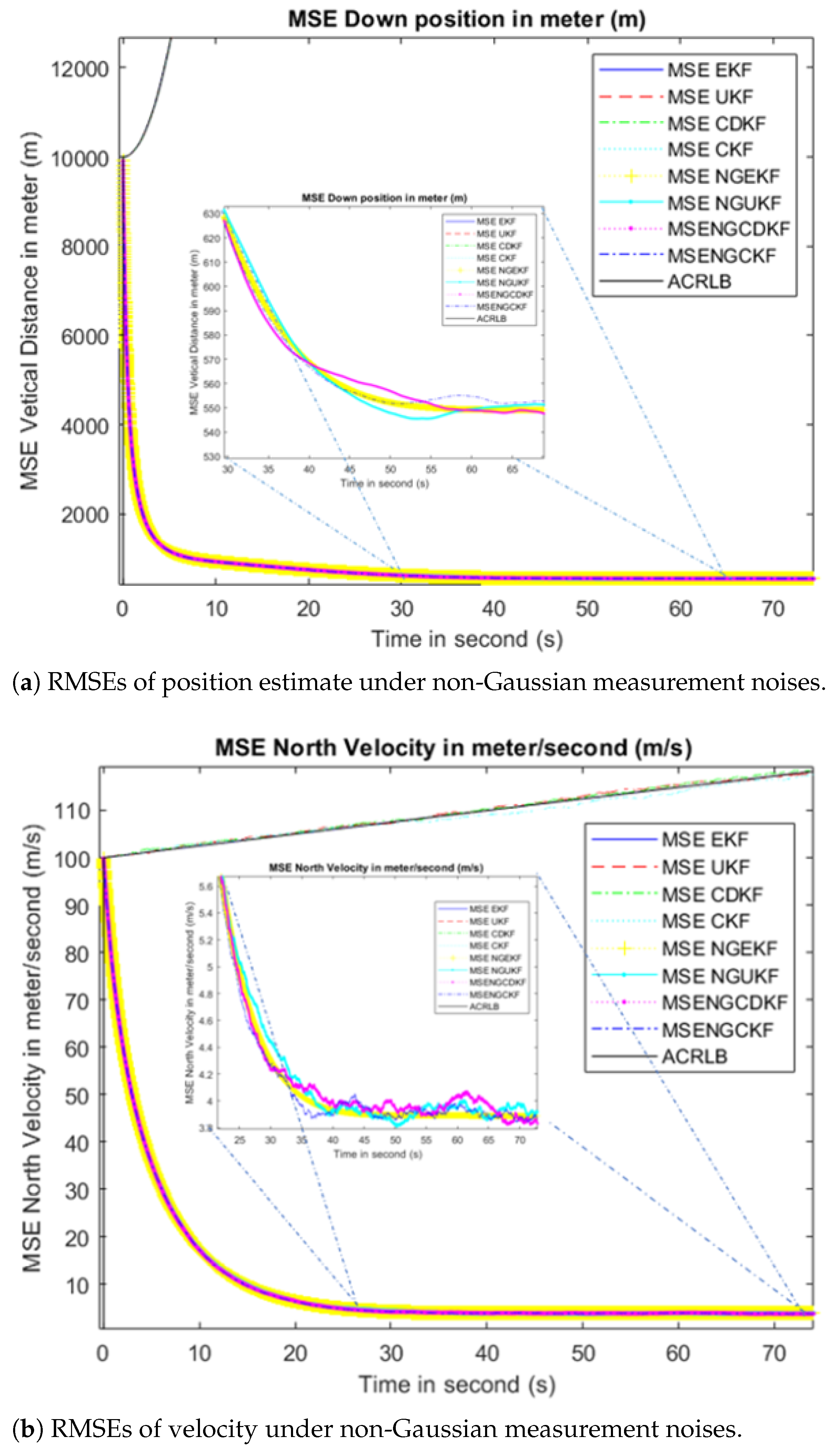
5.4. Cubature Kalman Filter (CKF)
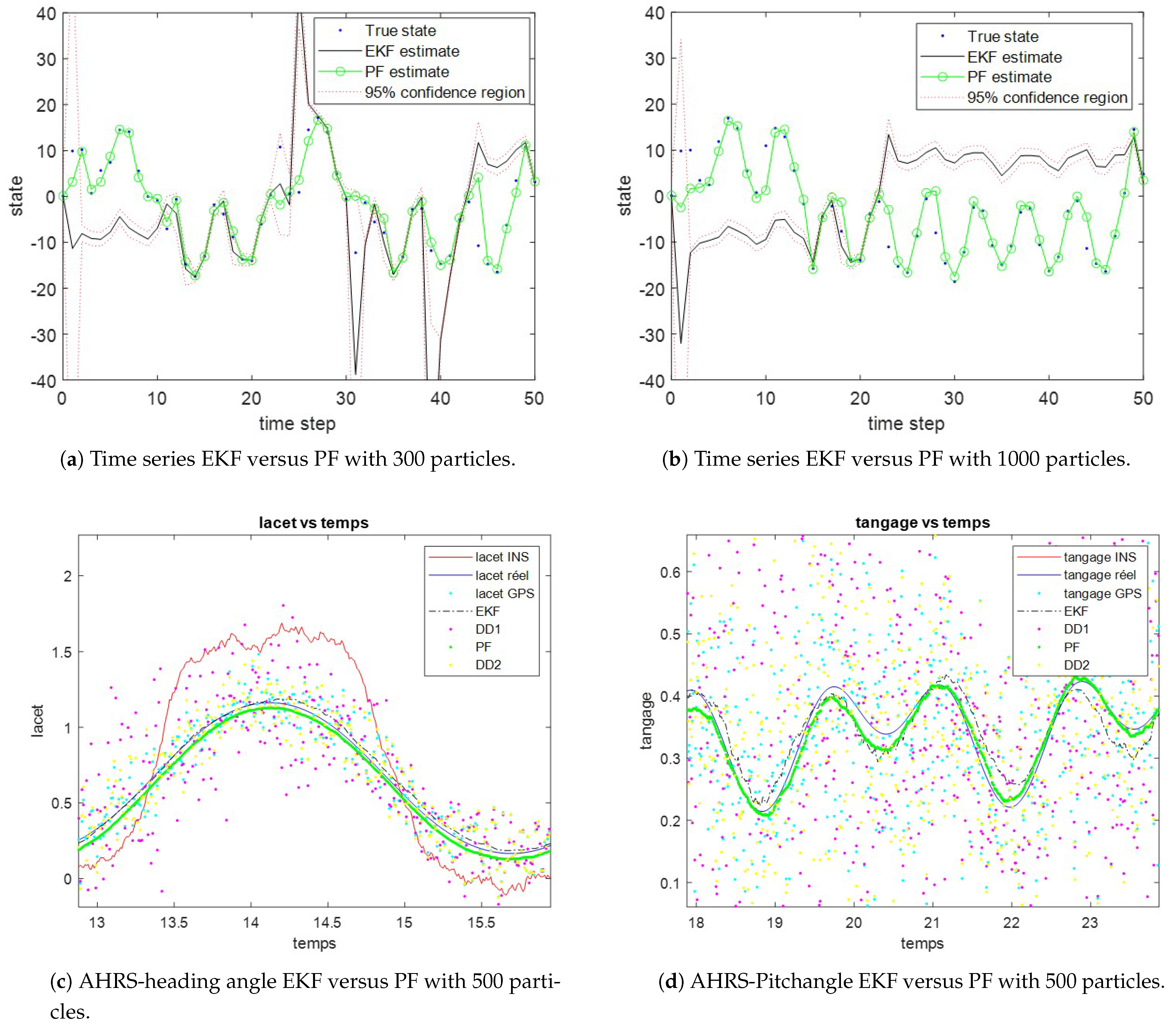
5.5. Particle Filter (PF)
5.6. Gaussian Mixture Model (GMM)
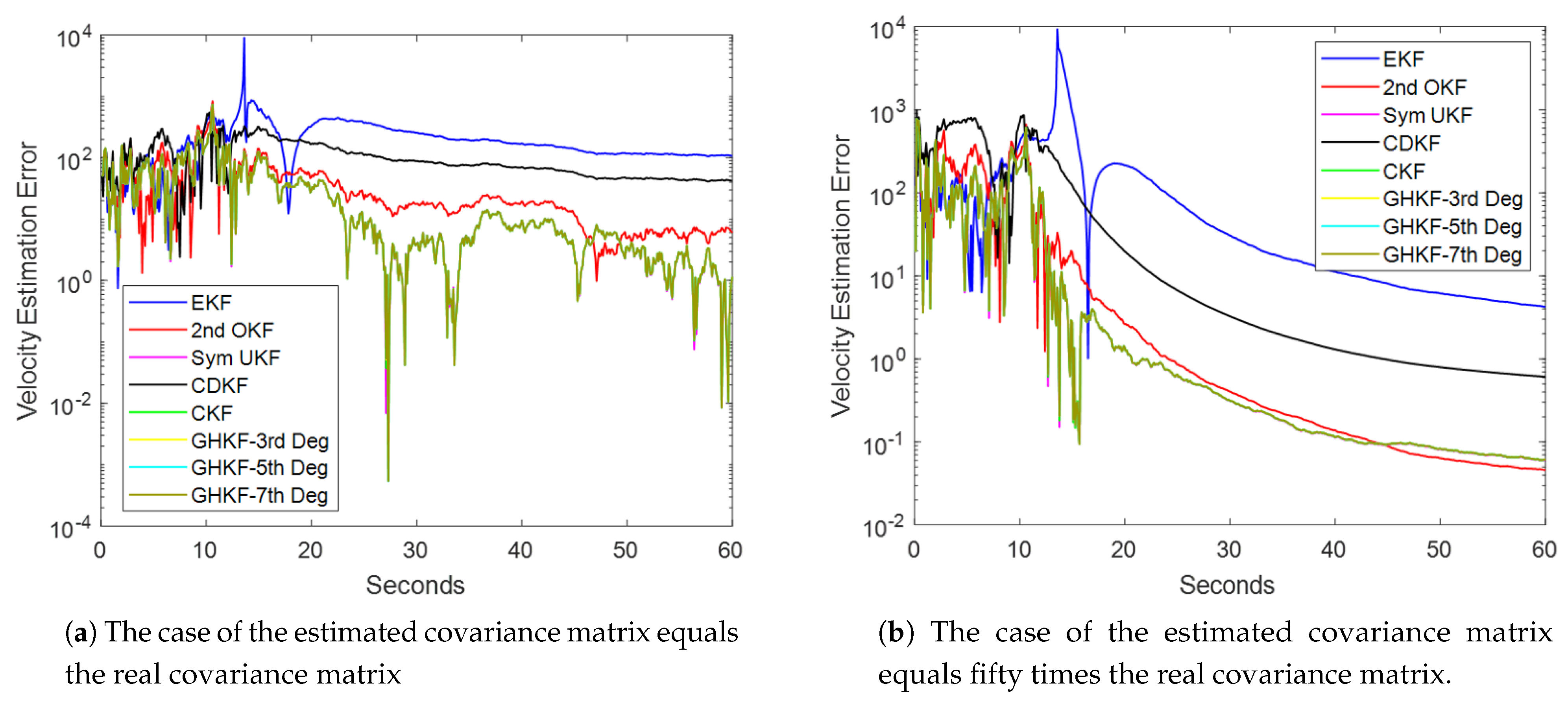
5.7. Multiple Quadrature Information Filters (MQIFs)
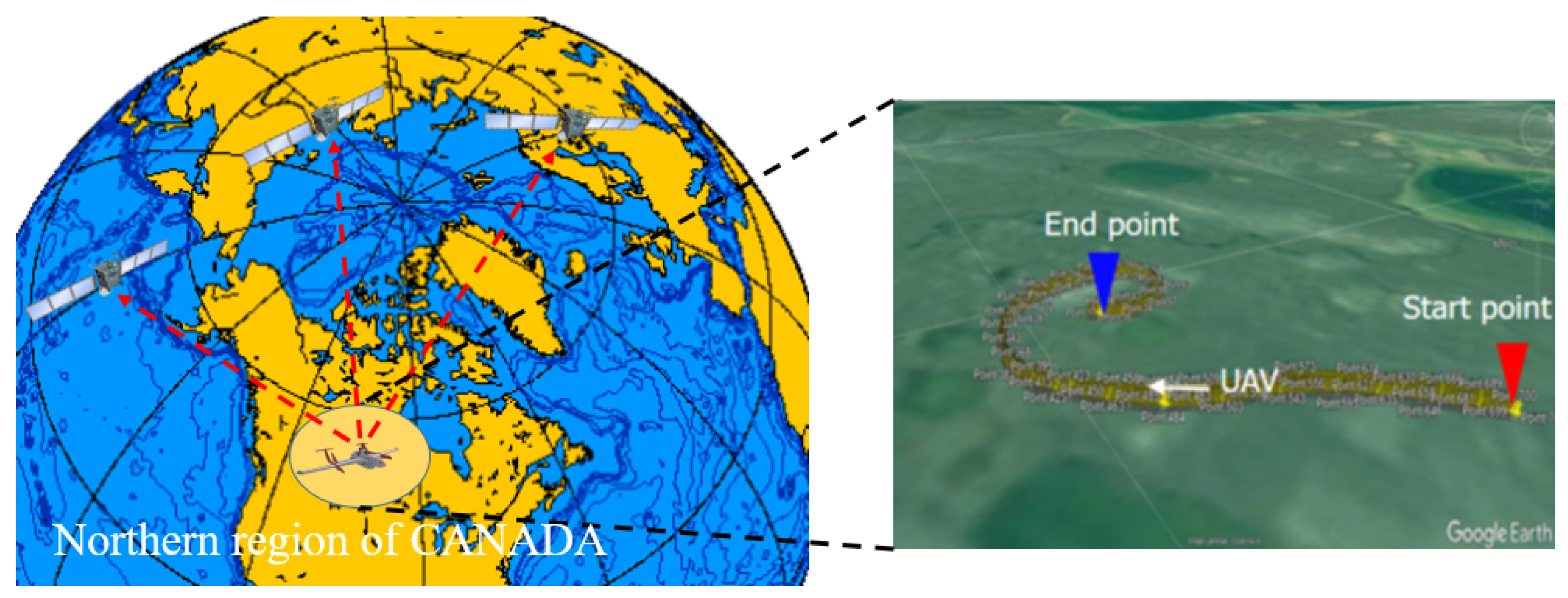
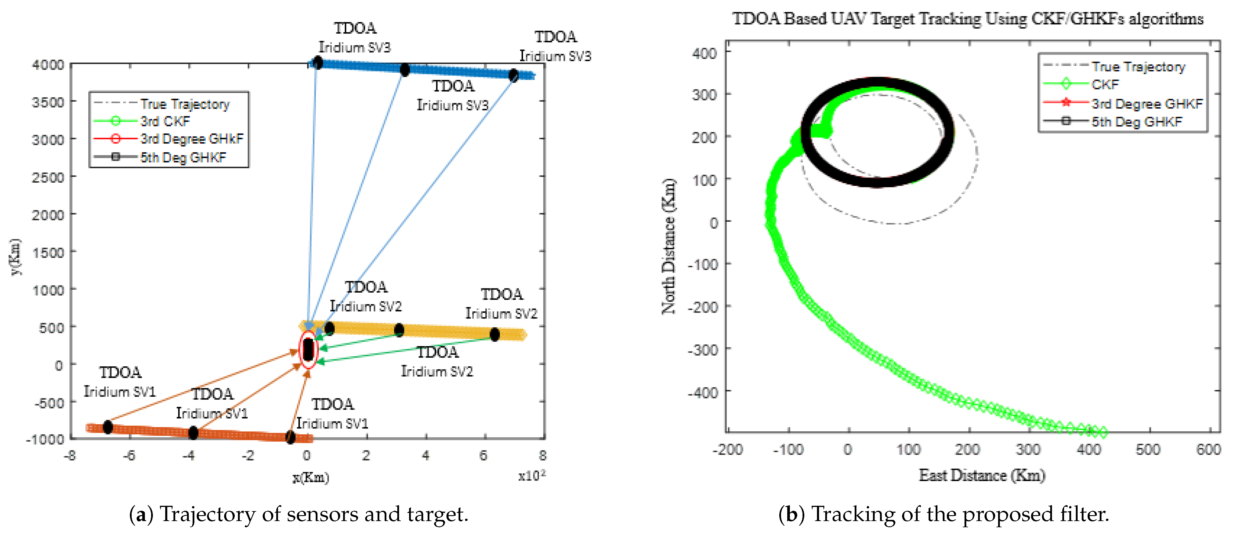
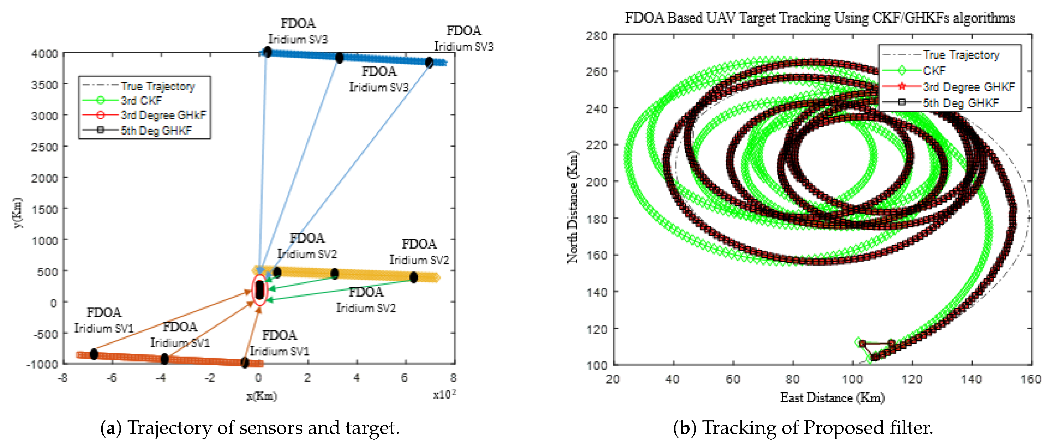
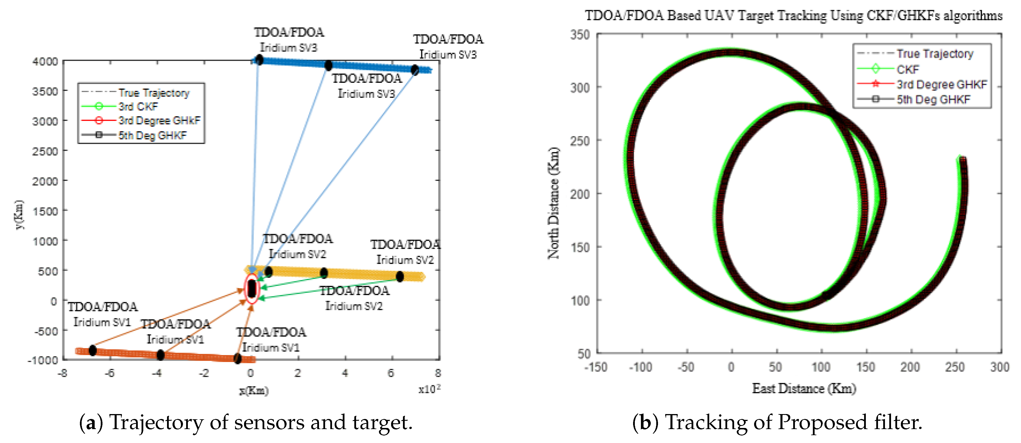
Scenario Simulation of RFI UAV Flying in the North Latitudes
5.8. Filter
5.9. Real Data Collection from GNSS Receivers and Sensors Fusion
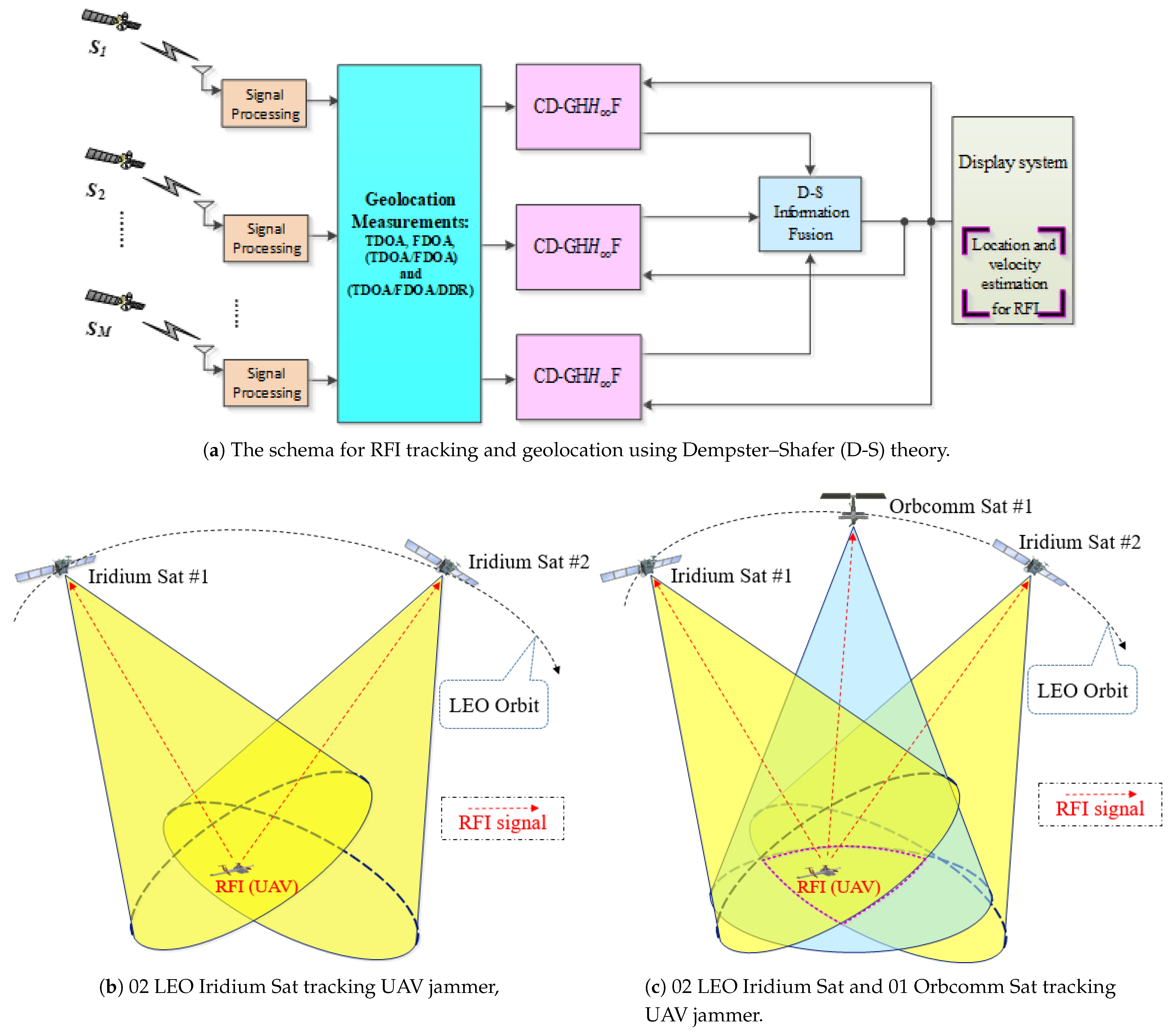
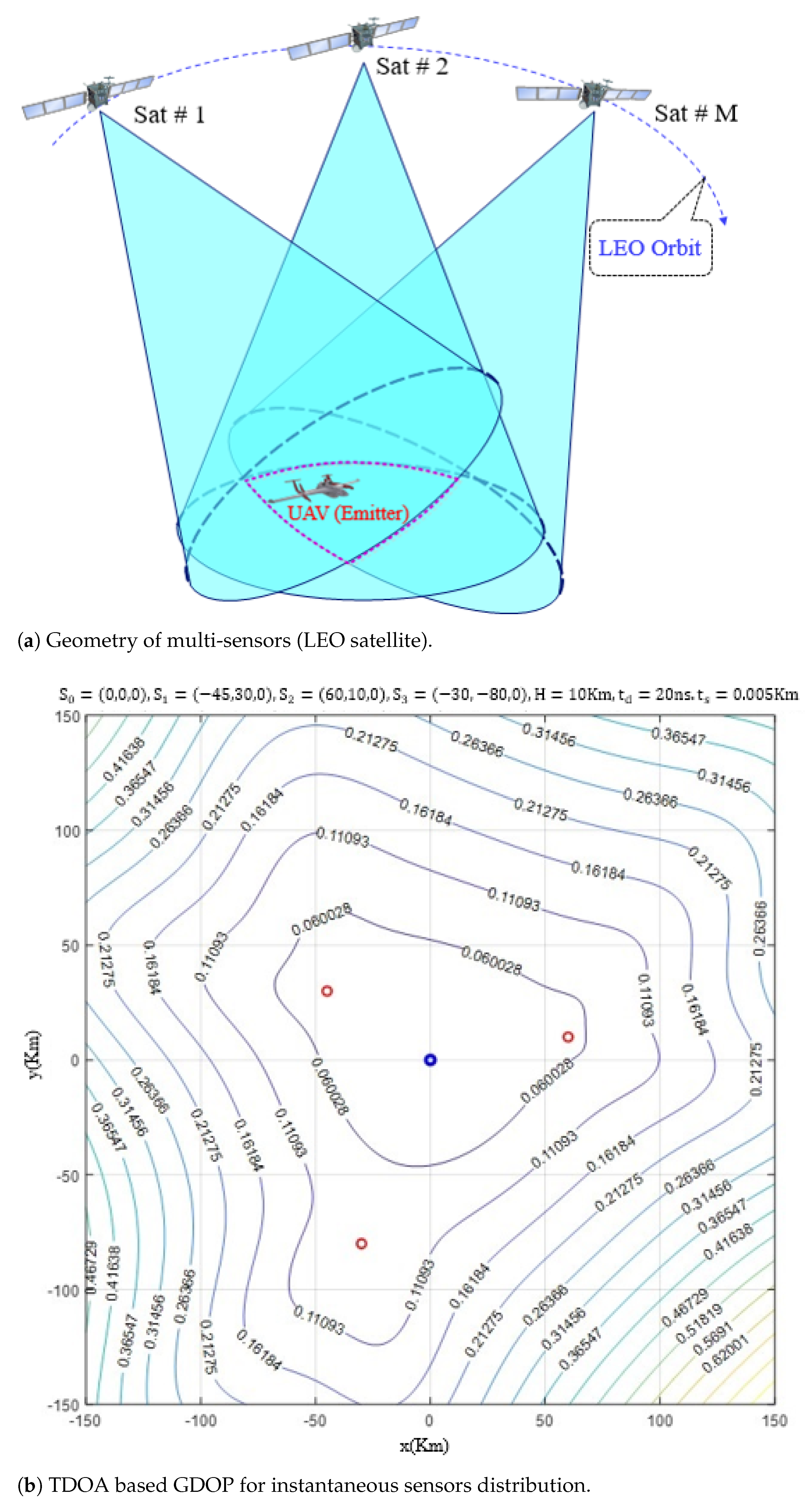
5.10. Real Data Collection from LEO Satellites
6. Conclusions
7. Future Works
- -
- The development of new numerical methods and non-linear approximation (deterministic and stochastic) integration carrying out faster convergence and numerical stability especially for the geolocation of stationary RFI.
- -
- The development of adaptive and learning monitoring of RFI signals parameters with simultaneous state and parameter learning algorithms, such as Gaussian processes, supervised and unsupervised techniques, etc.
- -
- The development of machine learning and artificial intelligence algorithms such as: reinforcement learning and information reinforcement learning (based on information theoretical learning) with partial knowledge or full unknown models for RFI detection, identification and tracking.
- -
- In addition, robust techniques such as the GHKF-H infinite presented and proposed should be optimized by using Fuzzy Logic for parameter tuning and other RL algorithms for best reactions to the environment uncertainty. To the best of our knowledge, this has not been done before in this field.
- -
- Another issue is the development of real-time implementation of all these algorithms, such as defining and classifying the best performances in real-time and their respective feasibility.To achieve this kind of classification, it might be interesting to propose a computational time complexity for each algorithm for each case study: stationary target, dynamical target, maneuvering target, stationary sensors network, mobile sensors network, LEO satellite sensors network.
- -
- More complex problems could be addressed by assuming multiple RFI-targets instead of only one, with multiple combinations of LEO satellite networks. The problem would be similar to multiple target tracking with only partial knowledge and uncertain data association algorithms to be developed.
- -
- An original and interesting problem would be optimal sensors placement, or optimal constellation selection for optimizing RFI-targets detection and tracking using and Gauss Hermite Quadrature filters package algorithms to overcome high non-linearity degrees and sensor locations uncertainty.
Author Contributions
Funding
Institutional Review Board Statement
Informed Consent Statement
Data Availability Statement
Conflicts of Interest
Abbreviations
| ADS-B | Automatic Dependent Surveillance-Broadcast |
| AEKF | Adaptive Extended Kalman Filter |
| AOA | Angle of Arrival |
| CAF | Cross Ambiguity Function |
| CAPITAL | Cellular Applied to IVHS Tracking and Location |
| CDFs | Cumulative Distribution Functions |
| CIR | Channel Impulse Response |
| CKF | Cubature Kalman Filter |
| CNN | Convolutional Neural Network |
| CRIAQ | Consortium for Research and Innovation in Aerospace in Quebec |
| CRLB | Cramér-Rao lower bound |
| CWLS | Constrained Weighted Least Square |
| DDR | Differential Doppler Rate |
| DL | Deep Learning |
| D-S | Dempster–Shafer |
| DVB | Digital Video Broadcasting |
| EKF | Extended Kalman Filter |
| EGNOS | European Geostationary Navigation Overlay Service |
| ÉTS | École de Technologie Supérieure |
| FDOA | Frequency Difference of Arrival |
| GA | Genetic Algorithm |
| GAGAN | GPS Aided Geo Augmented Navigation |
| GDOP | Geometric Dilution of Precision |
| GHKF | Gaussian Hermite Kalman Filter |
| GHQF | Gauss–Hermite Quadrature Filter |
| GLONASS | GLObal’naya NAvigatsioannaya Sputnikovaya Sistema |
| GMM | Gaussian Mixture Model |
| GMM-ITSF | Gaussian mixture measurement integrated track splitting filter |
| GMT | Ground Moving Targets |
| GNS | Navigation Systems |
| GNSS | Global Navigation Satellite Systems |
| GPS | Global Positioning System |
| GSN | GNSS Supervisory Authority |
| ICWLS | iterative constrained weighted least squares |
| INS | Inertial Navigation System |
| KF | Kalman Filtering |
| LASSENA | Laboratory of Space Technologies, Embedded System, Navigation and Avionic |
| LLS | Linear Least Squares |
| LOB | Line of Bearing |
| LOS | Line of Sigh |
| LS | Least Square |
| LSM | Least Square Methods |
| MAVs | Manned Aircraft Vehicles |
| ML | Maximum Likelihood |
| MLAT | Multilateration |
| MLE | Maximum Likelihood Estimator |
| MMF | multiple-model filter |
| MRPEs | mean relative position errors |
| MSPEs | mean square position errors |
| NLOS | Non-line of Sight |
| NLS | Non-linear Least Square |
| NSERC | Natural Sciences and Engineering Research Council of Canada |
| PDOA | Power Difference of Arrival |
| PF | Particle Filter |
| PNT | Positioning, Navigation, and Timing |
| QIKFs | Quadrature Information Kalman Filters |
| QKF | Quadrature Kalman filter |
| QLS | quadratic least squares |
| RFI | Radio-Frequency Interference |
| RMSE | Root Mean Square Error |
| RSS | Received Signal Strength |
| RTLS | Real-Time Locating System |
| SatCom | Satellite Communication |
| SBAS | Satellite Based Augmentation System |
| SDMC | System for Differential Correction and Monitoring |
| SDP | Semi-Definite Programming |
| SDR | Software-defined radios |
| SNR | Signal to the Noise ratio |
| SV | Space Vehicle |
| TDOA | Time Difference of Arrival |
| TLA | Tangent Linear Approximation |
| TOA | Time of Arrival |
| TS | Taylor Series |
| UAVs | Unmanned Aerial Vehicles |
| WAAS | Wide Area Augmentation System |
| WLS | Weighted Least Square |
| WSN | Wireless Sensor Networks |
References
- Kaiser, S.A.; Christianson, A.J.; Narayanan, R.M. Multistatic Doppler estimation using global positioning system passive coherent location. IEEE Trans. Aerosp. Electron. Syst. 2019, 55, 2978–2991. [Google Scholar] [CrossRef]
- Liu, W.; Ding, J.; Zheng, J.; Chen, X.; Chih-Lin, I. Relay-Assisted Technology in Optical Wireless Communications: A Survey. IEEE Access 2020, 8, 194384–194409. [Google Scholar] [CrossRef]
- Misra, D.; Misra, D.K.; Tripathi, S. Satellite communication advancement, issues, challenges and applications. Int. J. Adv. Res. Comput. Commun. Eng. 2013, 2, 1681–1686. [Google Scholar]
- Gilski, P.; Stefański, J. Survey of radio navigation systems. Int. J. Electron. Telecommun. 2014, 61, 43–48. [Google Scholar] [CrossRef]
- Morales-Ferre, R.; Richter, P.; Falletti, E.; de la Fuente, A.; Lohan, E.S. A survey on coping with intentional interference in satellite navigation for manned and unmanned aircraft. IEEE Commun. Surv. Tutor. 2019, 22, 249–291. [Google Scholar] [CrossRef]
- Carlo, D. GNSS Market Report Issue 5. Available online: http://www.gsa.europa.eu/gnss-market-report-issue-5-may-2017 (accessed on 1 May 2017).
- Jakhu, R.S. Satellites: Unintentional and Intentional Interference. In Proceedings of the Radio Frequency Interference and Space Sustainability, Washington, DC, USA, 17 June 2013. [Google Scholar]
- Wang, B.; Gan, X.; Liu, X.; Yu, B.; Jia, R.; Huang, L.; Jia, H. A novel weighted KNN algorithm based on RSS similarity and position distance for Wi-Fi fingerprint positioning. IEEE Access 2020, 8, 30591–30602. [Google Scholar] [CrossRef]
- Xiong, H.; Mai, Z.; Tang, J.; He, F. Robust GPS/INS/DVL navigation and positioning method using adaptive federated strong tracking filter based on weighted least square principle. IEEE Access 2019, 7, 26168–26178. [Google Scholar] [CrossRef]
- Zhang, S.; Pan, X.; Mu, H. A multi-pedestrian cooperative navigation and positioning method based on UWB technology. In Proceedings of the 2020 IEEE International Conference on Artificial Intelligence and Information Systems (ICAIIS), Dalian, China, 20–22 March 2020; pp. 260–264. [Google Scholar]
- Medina, D.A.; Romanovas, M.; Herrera-Pinzón, I.; Ziebold, R. Robust position and velocity estimation methods in integrated navigation systems for inland water applications. In Proceedings of the 2016 IEEE/ION Position, Location and Navigation Symposium (PLANS), Savannah, GA, USA, 11–16 April 2016; pp. 491–501. [Google Scholar]
- Tahat, A.; Kaddoum, G.; Yousefi, S.; Valaee, S.; Gagnon, F. A Look at the Recent Wireless Positioning Techniques With a Focus on Algorithms for Moving Receivers. IEEE Access 2016, 4, 6652–6680. [Google Scholar] [CrossRef]
- Gentile, C.; Alsindi, N.; Raulefs, R.; Teolis, C. Geolocation Techniques: Principles and Applications; Springer Science & Business Media: New York, NY, USA, 2012. [Google Scholar]
- Wu, P.; Su, S.; Zuo, Z.; Guo, X.; Sun, B.; Wen, X. Time difference of arrival (TDoA) localization combining weighted least squares and firefly algorithm. Sensors 2019, 19, 2554. [Google Scholar] [CrossRef] [PubMed]
- Noroozi, A.; Nayebi, M.M.; Amiri, R. Iterative constrained weighted least squares solution for target localization in distributed MIMO radar. In Proceedings of the 2019 27th Iranian Conference on Electrical Engineering (ICEE), Yazd, Iran, 30 April–2 May 2019; pp. 1710–1714. [Google Scholar]
- Hao, W.; Wei-min, S.; Hong, G. A novel Taylor series method for source and receiver localization using TDOA and FDOA measurements with uncertain receiver positions. In Proceedings of the 2011 IEEE CIE International Conference on Radar, Chengdu, China, 24–17 October 2011; Volume 2, pp. 1037–1040. [Google Scholar]
- Zhang, X.; Cui, Q.; Shi, Y.; Tao, X. Robust localisation algorithm for solving neighbour position ambiguity. Electron. Lett. 2013, 49, 1106–1107. [Google Scholar] [CrossRef]
- Chui, C.K.; Chen, G. Kalman Filtering; Springer: Berlin/Heidelberg, Germany, 2017. [Google Scholar]
- Pak, J.M.; Ahn, C.K.; Shmaliy, Y.S.; Lim, M.T. Improving reliability of particle filter-based localization in wireless sensor networks via hybrid particle/FIR filtering. IEEE Trans. Ind. Inform. 2015, 11, 1089–1098. [Google Scholar] [CrossRef]
- Benzerrouk, H. Modern Approaches in Nonlinear Filtering Theory Applied to Original Problems of Aerospace Integrated Navigation System with non-Gaussian Noise; Saint Petersburg State University: Sankt-Peterburg, Russia, 2014. [Google Scholar]
- Elgamoudi, A.; Benzerrouk, H.; Elango, G.A.; Landry, R. Gauss Hermite H∞ Filter for UAV Tracking Using LEO Satellites TDOA/FDOA Measurement—Part I. IEEE Access 2020, 8, 201428–201440. [Google Scholar] [CrossRef]
- Zhao, J.; Mili, L. A theoretical framework of robust H-infinity unscented Kalman filter and its application to power system dynamic state estimation. IEEE Trans. Signal Process. 2019, 67, 2734–2746. [Google Scholar] [CrossRef]
- Benzerrouk, H.; Nebylov, A.; Li, M. Multi-UAV Doppler information fusion for target tracking based on distributed high degrees information filters. Aerospace 2018, 5, 28. [Google Scholar] [CrossRef]
- Benzerrouk, H.; Nebylov, A.; Salhi, H. Contribution in information signal processing for solving state space nonlinear estimation problems. J. Signal Inf. Process. 2013, 4, 375–384. [Google Scholar] [CrossRef][Green Version]
- Cao, Y.C.; Fang, J.A. Constrained Kalman filter for localization and tracking based on TDOA and DOA measurements. In Proceedings of the 2009 International Conference on Signal Processing Systems, Singapore, 15–17 May 2009; pp. 28–33. [Google Scholar]
- Del Peral-Rosado, J.A.; Seco-Granados, G.; Kim, S.; López-Salcedo, J.A. Network design for accurate vehicle localization. IEEE Trans. Veh. Technol. 2019, 68, 4316–4327. [Google Scholar] [CrossRef]
- Wymeersch, H.; Seco-Granados, G.; Destino, G.; Dardari, D.; Tufvesson, F. 5G mmWave positioning for vehicular networks. IEEE Wirel. Commun. 2017, 24, 80–86. [Google Scholar] [CrossRef]
- Gezici, S. A survey on wireless position estimation. Wirel. Pers. Commun. 2008, 44, 263–282. [Google Scholar] [CrossRef]
- Sakpere, W.; Adeyeye-Oshin, M.; Mlitwa, N.B. A state-of-the-art survey of indoor positioning and navigation systems and technologies. S. Afr. Comput. J. 2017, 29, 145–197. [Google Scholar] [CrossRef]
- Simon, D. Optimal State Estimation: Kalman, H Infinity, and Nonlinear Approaches; John Wiley & Sons: Hoboken, NJ, USA, 2006. [Google Scholar]
- Wang, W.; Zhang, Y.; Tian, L. TOA-based NLOS error mitigation algorithm for 3D indoor localization. China Commun. 2020, 17, 63–72. [Google Scholar] [CrossRef]
- Tsivgoulis, G. Source Localization In Wireless Sensor Networks with Randomly Distributed Elements under Multipath Propagation Conditions; Technical Report; Naval Postgraduate School: Monterey, CA, USA, 2009. [Google Scholar]
- Fokin, G. TDOA Measurement Processing for Positioning in Non-Line-of-Sight Conditions. In Proceedings of the 2018 IEEE International Black Sea Conference on Communications and Networking (BlackSeaCom), Batumi, GA, USA, 4–7 June 2018; pp. 1–5. [Google Scholar]
- Kim, J. Non-line-of-sight error mitigating algorithms for transmitter localization based on hybrid TOA/RSSI measurements. Wirel. Netw. 2020, 26, 3629–3635. [Google Scholar] [CrossRef]
- Ho, T.J. Intelligent M-Robust Extended Kalman Filtering for Mobile Tracking. In Proceedings of the 2019 IEEE International Conference on Systems, Man and Cybernetics (SMC), Bari, Italy, 6–9 October 2019; pp. 2332–2337. [Google Scholar]
- N de Sousa, M.; S Thomä, R. Enhancement of localization systems in NLOS urban scenario with multipath ray tracing fingerprints and machine learning. Sensors 2018, 18, 4073. [Google Scholar] [CrossRef] [PubMed]
- Aghaie, N.; Tinati, M.A. Localization of WSN nodes based on NLOS identification using AOAs statistical information. In Proceedings of the 2016 24th Iranian Conference on Electrical Engineering (ICEE), Shiraz, Iran, 10–12 May 2016; pp. 496–501. [Google Scholar]
- He, C.; Guo, F.; Li, X.; Zhang, M. Bias Analysis of AOA-Based Geolocation. In Proceedings of the 2018 2nd IEEE Advanced Information Management, Communicates, Electronic and Automation Control Conference (IMCEC), Xi’an, China, 25–27 May 2018; pp. 1711–1715. [Google Scholar]
- Wang, Y.; Ho, K. An asymptotically efficient estimator in closed-form for 3-D AOA localization using a sensor network. IEEE Trans. Wirel. Commun. 2015, 14, 6524–6535. [Google Scholar] [CrossRef]
- Choi, S.; Cha, J. Performance analysis of the jamming signal geolocation system using on-board AoA estimator mounted on UAV. In Proceedings of the 2017 17th International Conference on Control, Automation and Systems (ICCAS), Jeju, Korea, 18–21 October 2017; pp. 1976–1979. [Google Scholar]
- Zheng, Y.; Sheng, M.; Liu, J.; Li, J. Exploiting AoA estimation accuracy for indoor localization: A weighted AoA-based approach. IEEE Wirel. Commun. Lett. 2018, 8, 65–68. [Google Scholar] [CrossRef]
- Gezici, S.; Tian, Z.; Giannakis, G.B.; Kobayashi, H.; Molisch, A.F.; Poor, H.V.; Sahinoglu, Z. Localization via ultra-wideband radios: A look at positioning aspects for future sensor networks. IEEE Signal Process. Mag. 2005, 22, 70–84. [Google Scholar] [CrossRef]
- Liang, K.; Huang, Z.; He, J. A passive localization method of single satellite using TOA sequence. In Proceedings of the 2016 2nd IEEE International Conference on Computer and Communications (ICCC), Chengdu, China, 14–17 October 2016; pp. 1795–1798. [Google Scholar]
- Ho, K.; Lu, X.; Kovavisaruch, L.O. Source localization using TDOA and FDOA measurements in the presence of receiver location errors: Analysis and solution. IEEE Trans. Signal Process. 2007, 55, 684–696. [Google Scholar] [CrossRef]
- Sun, Y.; Ho, K.; Wan, Q. Solution and analysis of TDOA localization of a near or distant source in closed form. IEEE Trans. Signal Process. 2018, 67, 320–335. [Google Scholar] [CrossRef]
- Meng, Y.; Xu, J.; Huang, Y.; He, J. Key factors of multi-station TDOA passive location study. In Proceedings of the 2015 7th International Conference on Intelligent Human-Machine Systems and Cybernetics, Hangzhou, China, 26–27 August 2015; Volume 2, pp. 220–223. [Google Scholar]
- Zhang, C.; Qin, N.; Xue, Y.; Yang, L. Received signal strength-based indoor localization using hierarchical classification. Sensors 2020, 20, 1067. [Google Scholar] [CrossRef] [PubMed]
- Basar, E.; Di Renzo, M.; De Rosny, J.; Debbah, M.; Alouini, M.S.; Zhang, R. Wireless communications through reconfigurable intelligent surfaces. IEEE Access 2019, 7, 116753–116773. [Google Scholar] [CrossRef]
- Ciuonzo, D.; Rossi, P.S.; Willett, P. Generalized Rao test for decentralized detection of an uncooperative target. IEEE Signal Process. Lett. 2017, 24, 678–682. [Google Scholar] [CrossRef]
- Shoari, A.; Seyedi, A. Detection of a non-cooperative transmitter in Rayleigh fading with binary observations. In Proceedings of the MILCOM 2012—2012 IEEE Military Communications Conference, Orlando, FL, USA, 29 October–1 November 2012; pp. 1–5. [Google Scholar]
- Blay, R.C.; Akos, D.M. GNSS RFI localization using a hybrid TDOA/PDOA approach. In Proceedings of the 2018 International Technical Meeting of The Institute of Navigation, Reston, VA, USA, 19 January 2018; pp. 703–712. [Google Scholar]
- Tucker, J.A.; Puskar, C.; Lee, C.; Akos, D. GPS/GNSS Interference Power Difference of Arrival (PDOA) Localization Weighted via Nearest Neighbors. In Proceedings of the 33rd International Technical Meeting of the Satellite Division of The Institute of Navigation (ION GNSS+ 2020), Online, 21–25 September 2020; pp. 3550–3560. [Google Scholar]
- Guo, S.; Jackson, B.; Wang, S.; Inkol, R.; Arnold, W. A novel density-based geolocation algorithm for a noncooperative radio emitter using power difference of arrival. In Proceedings of the SPIE Defense, Security, and Sensing, Orlando, FL, USA, 25–29 April 2011; Volume 8061, p. 80610E. [Google Scholar]
- He, L.; Li, H.; Lu, M. Dual-antenna GNSS spoofing detection method based on Doppler frequency difference of arrival. GPS Solut. 2019, 23, 78. [Google Scholar] [CrossRef]
- Broad, J.T.; Savage, L.M. Frequency Difference of Arrival (FDOA) for Geolocation. U.S. Patent 9,702,960, 11 July 2017. [Google Scholar]
- Vesely, J. Differential doppler target position fix computing methods. In Proceedings of the International Conference on Circuits, Systems, Signals, San Francisco, CA, USA, 22–24 October 2019; pp. 284–287. [Google Scholar]
- Landry, R.; Nguyen, A.; Rasaee, H.; Amrhar, A.; Fang, X.; Benzerrouk, H. Iridium Next LEO satellites as an alternative PNT in GNSS denied environments—Part 1. Inside GNSS Mag. 2019, 56–64. [Google Scholar]
- O’Donoughue, N. Emitter Detection and Geolocation for Electronic Warfare; Artech House: Norwood, MA, USA, 2019. [Google Scholar]
- Zhao, Y.; Qi, W.; Liu, P.; Chen, L.; Lin, J. Accurate 3D localisation of mobile target using single station with AoA–TDoA measurements. IET Radar Sonar Navig. 2020, 14, 954–965. [Google Scholar] [CrossRef]
- Aernouts, M.; BniLam, N.; Podevijn, N.; Plets, D.; Joseph, W.; Berkvens, R.; Weyn, M. Combining TDoA and AoA with a particle filter in an outdoor LoRaWAN network. In Proceedings of the 2020 IEEE/ION Position, Location and Navigation Symposium (PLANS), Portland, OR, USA, 20–23 April 2020; pp. 1060–1069. [Google Scholar]
- Chen, H.; Ballal, T.; Saeed, N.; Alouini, M.S.; Al-Naffouri, T.Y. A Joint TDOA-PDOA Localization Approach Using Particle Swarm Optimization. IEEE Wirel. Commun. Lett. 2020, 9, 1240–1244. [Google Scholar] [CrossRef]
- Kim, D.G.; Park, G.H.; Kim, H.N.; Park, J.O.; Park, Y.M.; Shin, W.H. Computationally efficient TDOA/FDOA estimation for unknown communication signals in electronic warfare systems. IEEE Trans. Aerosp. Electron. Syst. 2017, 54, 77–89. [Google Scholar] [CrossRef]
- Akos, D.M.; Blay, R.; Shivaramaiah, N.C. Hybrid Interference Localization. U.S. Patent Application 16/246,177, 18 July 2019. [Google Scholar]
- Zhao, Y.; Li, Z.; Hao, B.; Wan, P.; Wang, L. How to select the best sensors for TDOA and TDOA/AOA localization? China Commun. 2019, 16, 134–145. [Google Scholar]
- Yin, S.; Chen, D.; Zhang, Q.; Liu, M.; Li, S. Mining spectrum usage data: A large-scale spectrum measurement study. IEEE Trans. Mob. Comput. 2012, 11, 1033–1046. [Google Scholar]
- Zhao, Y.; Lung, C.H.; Lambadaris, I.; Goel, N. A hybrid location identification method in wireless AD Hoc/sensor networks. In Proceedings of the 2009 Tenth International Conference on Mobile Data Management: Systems, Services and Middleware, Taipei, Taiwan, 18–21 May 2009; pp. 465–473. [Google Scholar]
- Yin, J.; Wan, Q.; Yang, S.; Ho, K. A simple and accurate TDOA-AOA localization method using two stations. IEEE Signal Process. Lett. 2015, 23, 144–148. [Google Scholar] [CrossRef]
- Nur-A-Alam, M.; Haque, M.M. A least square approach for tdoa/aoa wireless location in wcdma system. In Proceedings of the 2008 11th International Conference on Computer and Information Technology, Nadi, Fiji, 8–10 December 2016; pp. 686–690. [Google Scholar]
- Li, W.; Liu, P. 3D AOA/TDOA emitter location by integrated passive radar/GPS/INS systems. In Proceedings of the 2005 IEEE International Workshop on VLSI Design and Video Technology, Suzhou, China, 28–30 May 2005; pp. 121–124. [Google Scholar]
- Overfield, J.; Biskaduros, Z.; Buehrer, R.M. Geolocation of MIMO signals using the cross ambiguity function and TDOA/FDOA. In Proceedings of the 2012 IEEE International Conference on Communications (ICC), Ottawa, ON, Canada, 10–15 June 2012; pp. 3648–3653. [Google Scholar]
- Abbasbandy, S. Improving Newton–Raphson method for nonlinear equations by modified Adomian decomposition method. Appl. Math. Comput. 2003, 145, 887–893. [Google Scholar] [CrossRef]
- Elgamoudi, A.; Shahzad, A.; Landry, R. Contribution to develop a generic hybrid technique of satellite system for RFI geolocation. In Proceedings of the 2017 14th International Bhurban Conference on Applied Sciences and Technology (IBCAST), Islamabad, Pakistan, 10–14 January 2017; pp. 764–771. [Google Scholar]
- Yatrakis, C.L. Computing the Cross Ambiguity Function oe A Review. Ph.D. Thesis, State University of New York, New York, NY, USA, 2005. [Google Scholar]
- Deng, B.; Sun, Z.B.; Peng, H.F.; Xiong, J.Y. Source localization using TDOA/FDOA/DFS measurements with erroneous sensor positions. In Proceedings of the 2016 CIE International Conference on Radar (RADAR), Guangzhou, China, 10–13 October 2016; pp. 1–4. [Google Scholar]
- Liu, Z.; Hu, D.; Zhao, Y.; Zhao, Y. An algebraic method for moving source localization using TDOA, FDOA, and differential Doppler rate measurements with receiver location errors. EURASIP J. Adv. Signal Process. 2019, 2019, 25. [Google Scholar] [CrossRef]
- Hu, D.; Luo, L.; Huang, D.; Chen, S. A Joint TDOA, FDOA and Doppler Rate Parameters Estimation Method and Its Performance Analysis. In Proceedings of the 2019 IEEE 21st International Conference on High Performance Computing and Communications; IEEE 17th International Conference on Smart City; IEEE 5th International Conference on Data Science and Systems (HPCC/SmartCity/DSS), Zhangjiajie, China, 10–12 August 2019; pp. 2482–2486. [Google Scholar]
- Zekavat, R.; Buehrer, R.M. Handbook of Position Location: Theory, Practice and Advances; John Wiley & Sons: Hoboken, NJ, USA, 2011; Volume 27. [Google Scholar]
- Series, S. Comparison of Time-Difference-of-Arrival and Angle-of-Arrival Methods of Signal Geolocation; ITU: Geneva, Switzerland, 2011. [Google Scholar]
- Podevijn, N.; Plets, D.; Trogh, J.; Martens, L.; Suanet, P.; Hendrikse, K.; Joseph, W. TDoA-based outdoor positioning with tracking algorithm in a public LoRa network. Wirel. Commun. Mob. Comput. 2018, 2018. [Google Scholar] [CrossRef]
- Li, X.; Deng, Z.D.; Rauchenstein, L.T.; Carlson, T.J. Contributed Review: Source-localization algorithms and applications using time of arrival and time difference of arrival measurements. Rev. Sci. Instrum. 2016, 87, 041502. [Google Scholar] [CrossRef]
- Hu, D.; Chen, S.; Bai, H.; Zhao, C.; Luo, L. CRLB for joint estimation of TDOA, phase, FDOA, and Doppler rate. J. Eng. 2019, 2019, 7628–7631. [Google Scholar] [CrossRef]
- Lu, J.; Yang, X. Taylor Series Localization Algorithm Based on Semi-definite Programming. In Proceedings of the International Conference on Artificial Intelligence and Security, New York, NY, USA, 26–28 July 2019; pp. 488–497. [Google Scholar]
- Ren, J.; Chen, J.; Bai, W. A new localization algorithm based on Taylor series expansion for NLOS environment. Cybern. Inf. Technol. 2016, 16, 127–136. [Google Scholar] [CrossRef]
- Rossi, R.J. Mathematical Statistics: An Introduction to Likelihood Based Inference; John Wiley & Sons: Hoboken, NJ, USA, 2018. [Google Scholar]
- Jia, T.; Shen, X.; Wang, H. Multistatic sonar localization with a transmitter. IEEE Access 2019, 7, 111192–111203. [Google Scholar] [CrossRef]
- Watanabe, F. Wireless Sensor Network Localization Using AoA Measurements with Two-Step Error Variance-Weighted Least Squares. IEEE Access 2021, 9, 10820–10828. [Google Scholar] [CrossRef]
- Wang, Y. Linear least squares localization in sensor networks. Eurasip J. Wirel. Commun. Netw. 2015, 2015, 1–7. [Google Scholar] [CrossRef]
- Dardari, D.; Falletti, E.; Luise, M. Satellite and Terrestrial Radio Positioning Techniques: A Signal Processing Perspective; Academic Press: Cambridge, MA, USA, 2012. [Google Scholar]
- Kang, S.; Kim, T.; Chung, W. Hybrid RSS/AOA Localization using Approximated Weighted Least Square in Wireless Sensor Networks. Sensors 2020, 20, 1159. [Google Scholar] [CrossRef] [PubMed]
- Wang, D.; Zhang, P.; Yang, Z.; Wei, F.; Wang, C. A novel estimator for TDOA and FDOA positioning of multiple disjoint sources in the presence of calibration emitters. IEEE Access 2019, 8, 1613–1643. [Google Scholar] [CrossRef]
- Cheung, K.W.; So, H.C. A multidimensional scaling framework for mobile location using time-of-arrival measurements. IEEE Trans. Signal Process. 2005, 53, 460–470. [Google Scholar] [CrossRef]
- Díez-González, J.; Álvarez, R.; González-Bárcena, D.; Sánchez-González, L.; Castejón-Limas, M.; Perez, H. Genetic algorithm approach to the 3D node localization in TDOA systems. Sensors 2019, 19, 3880. [Google Scholar] [CrossRef] [PubMed]
- Beynon, M.; Curry, B.; Morgan, P. The Dempster–Shafer theory of evidence: An alternative approach to multicriteria decision modelling. Omega 2000, 28, 37–50. [Google Scholar] [CrossRef]
- O’Shea, T.J.; Roy, T.; Clancy, T.C. Over-the-air deep learning based radio signal classification. IEEE J. Sel. Top. Signal Process. 2018, 12, 168–179. [Google Scholar] [CrossRef]
- Chang, Y.T.; Wu, C.L.; Cheng, H.C. The Enhanced Locating Performance of an Integrated Cross-Correlation and Genetic Algorithm for Radio Monitoring Systems. Sensors 2014, 14, 7541–7562. [Google Scholar] [CrossRef] [PubMed]
- Challa, S.; Koks, D. Bayesian and dempster-shafer fusion. Sadhana 2004, 29, 145–174. [Google Scholar] [CrossRef]
- Van Nguyen, T.; Jeong, Y.; Shin, H.; Win, M.Z. Machine learning for wideband localization. IEEE J. Sel. Areas Commun. 2015, 33, 1357–1380. [Google Scholar] [CrossRef]
- Schmidhuber, J. Deep learning in neural networks: An overview. Neural Netw. 2015, 61, 85–117. [Google Scholar] [CrossRef]
- Bengio, Y.; Courville, A.; Vincent, P. Representation learning: A review and new perspectives. IEEE Trans. Pattern Anal. Mach. Intell. 2013, 35, 1798–1828. [Google Scholar] [CrossRef]
- Niitsoo, A.; Edelhäußer, T.; Eberlein, E.; Hadaschik, N.; Mutschler, C. A deep learning approach to position estimation from channel impulse responses. Sensors 2019, 19, 1064. [Google Scholar] [CrossRef]
- Foy, W.H. Position-location solutions by Taylor-series estimation. IEEE Trans. Aerosp. Electron. Syst. 1976, AES-12, 187–194. [Google Scholar] [CrossRef]
- Fu, S.; Li, Y.; Zhang, M.; Zong, K.; Cheng, L.; Wu, M. Ultra-wideband pose detection system for boom-type roadheader based on Caffery transform and Taylor series expansion. Meas. Sci. Technol. 2017, 29, 015101. [Google Scholar] [CrossRef]
- Mehboob, U.; Qadir, J.; Ali, S.; Vasilakos, A. Genetic algorithms in wireless networking: Techniques, applications, and issues. Soft Comput. 2016, 20, 2467–2501. [Google Scholar] [CrossRef]
- NIST. Engineering Statistics, Handbook. Available online: https://www.itl.nist.gov/div898/handbook/eda/section3/eda3652.htm (accessed on 18 January 2021).
- Pajares, A.; Blasco, X.; Herrero, J.M.; Reynoso-Meza, G. A multiobjective genetic algorithm for the localization of optimal and nearly optimal solutions which are potentially useful: NevMOGA. Complexity 2018, 2018, 1792420. [Google Scholar] [CrossRef]
- Yang, X.S. Nature-Inspired Optimization Algorithms; Academic Press: Cambridge, MA, USA, 2020. [Google Scholar]
- Kim, Y.; Bang, H. Introduction to Kalman filter and its applications. In Introduction and Implementations of the Kalman Filter; IntechOpen: London, UK, 2018. [Google Scholar]
- Pititeeraphab, Y.; Jusing, T.; Chotikunnan, P.; Thongpance, N.; Lekdee, W.; Teerasoradech, A. The effect of average filter for complementary filter and Kalman filter based on measurement angle. In Proceedings of the 2016 9th Biomedical Engineering International Conference (BMEiCON), Luang Prabang, Laos, 7–9 December 2016; pp. 1–4. [Google Scholar]
- Zhao, D.; Sun, J.; Gui, G. En-route Multilateration System Based on ADS-B and TDOA/AOA for Flight Surveillance Systems. In Proceedings of the 2020 IEEE 91st Vehicular Technology Conference (VTC2020-Spring), Antwerp, Begium, 25–28 May 2020; pp. 1–6. [Google Scholar]
- Kim, D.; Ha, J.; You, K. Adaptive extended Kalman filter based geolocation using TDOA/FDOA. Int. J. Control Autom. 2011, 4, 49–58. [Google Scholar]
- Fu, K.; Zhang, D.; Tang, P.; Tang, Z.; He, W. Adaptive extended Kalman filter for a red shift navigation system. In Proceedings of the 2015 34th Chinese Control Conference (CCC), Hangzhou, China, 28–30 July 2015; pp. 5194–5199. [Google Scholar]
- Chen, Y.M.; Tsai, C.L.; Fang, R.W. TDOA/FDOA mobile target localization and tracking with adaptive extended Kalman filter. In Proceedings of the 2017 International Conference on Control, Artificial Intelligence, Robotics & Optimization (ICCAIRO), Prague, Czech Republic, 22–17 May 2017; pp. 202–206. [Google Scholar]
- MathWork. Radar Tracking. Available online: https://www.mathworks.com/help/dsp/ug/radar-tracking.html (accessed on 18 April 2021).
- Arasaratnam, I.; Haykin, S.; Hurd, T.R. Cubature Kalman filtering for continuous-discrete systems: Theory and simulations. IEEE Trans. Signal Process. 2010, 58, 4977–4993. [Google Scholar] [CrossRef]
- Arasaratnam, I.; Haykin, S. Cubature kalman filters. IEEE Trans. Autom. Control 2009, 54, 1254–1269. [Google Scholar] [CrossRef]
- Benzerrouk, H.; Nebylov, A.; Salhi, H. Quadrotor UAV state estimation based on High-Degree Cubature Kalman filter. IFAC-PapersOnLine 2016, 49, 349–354. [Google Scholar] [CrossRef]
- Jin, S.; Huang, H.; Li, Y.; Ren, Y.; Wang, Y.; Zhong, R. An Improved Particle Filter Based Track-Before-Detect Method for Underwater Target Bearing Tracking. In Proceedings of the OCEANS 2019-Marseille, Marseille, France, 17–20 June 2019; pp. 1–5. [Google Scholar]
- Mihaylova, L.; Angelova, D.; Honary, S.; Bull, D.R.; Canagarajah, C.N.; Ristic, B. Mobility tracking in cellular networks using particle filtering. IEEE Trans. Wirel. Commun. 2007, 6, 3589–3599. [Google Scholar] [CrossRef]
- Del Moral, P. Nonlinear filtering: Interacting particle resolution. C. R. L’Acad. Sci.-Ser. I-Math. 1997, 325, 653–658. [Google Scholar] [CrossRef]
- Cho, J.A.; Na, H.; Kim, S.; Ahn, C. Moving-target tracking based on particle filter with TDOA/FDOA measurements. Etri J. 2012, 34, 260–263. [Google Scholar] [CrossRef]
- Reynolds, D.A. Gaussian Mixture Models. Encycl. Biom. 2009, 741, 659–663. [Google Scholar]
- Okello, N.; Fletcher, F.; Musicki, D.; Ristic, B. Comparison of recursive algorithms for emitter localisation using TDOA measurements from a pair of UAVs. IEEE Trans. Aerosp. Electron. Syst. 2011, 47, 1723–1732. [Google Scholar] [CrossRef]
- Arasaratnam, I.; Haykin, S. Square-root quadrature Kalman filtering. IEEE Trans. Signal Process. 2008, 56, 2589–2593. [Google Scholar] [CrossRef]
- Closas, P.; Fernandez-Prades, C.; Vila-Valls, J. Multiple quadrature Kalman filtering. IEEE Trans. Signal Process. 2012, 60, 6125–6137. [Google Scholar] [CrossRef]
- Zhao, J.; Mili, L. A decentralized H-infinity unscented Kalman filter for dynamic state estimation against uncertainties. IEEE Trans. Smart Grid 2018, 10, 4870–4880. [Google Scholar] [CrossRef]
- Wang, Q.; Li, J.; Zhang, M.; Yang, C. H-infinity filter based particle filter for maneuvering target tracking. Prog. Electromagn. Res. 2011, 30, 103–116. [Google Scholar] [CrossRef]
- Ting Goh, S.; Zekavat, S.; Abdelkhalik, O. An Introduction to Kalman Filtering Implementation for Localization and Tracking Applications. In Handbook of Position Location: Theory, Practice, and Advances, 2nd ed.; John Wiley & Sons: Hoboken, NJ, USA, 2018; pp. 143–195. [Google Scholar]
- Jokić, I.; Zečević, Ž.; Krstajić, B. State-of-charge estimation of lithium-ion batteries using extended Kalman filter and unscented Kalman filter. In Proceedings of the 2018 23rd International Scientific-Professional Conference on Information Technology (IT), Žabljak, Montenegro, 19–24 February 2018; pp. 1–4. [Google Scholar]
- Zhang, W.; Gu, W.; Chen, C.; Chowdhury, M.; Kavehrad, M. Gaussian mixture sigma-point particle filter for optical indoor navigation system. In Proceedings of the SPIE OPTO 2014, San Francisco, CA, USA, 1–6 February 2014; Volume 9007, p. 90070K. [Google Scholar]
- Nguyen, T. Gaussian Mixture Model Based Spatial Information Concept for Image Segmentation; University of Windsor: Windsor, ON, Canada, 2011. [Google Scholar]
- Ke, D.; Chung, C.; Sun, Y. A novel probabilistic optimal power flow model with uncertain wind power generation described by customized Gaussian mixture model. IEEE Trans. Sustain. Energy 2015, 7, 200–212. [Google Scholar] [CrossRef]
- Arasaratnam, I.; Haykin, S.; Elliott, R.J. Discrete-time nonlinear filtering algorithms using Gauss–Hermite quadrature. Proc. IEEE 2007, 95, 953–977. [Google Scholar] [CrossRef]
- Díez-González, J.; Álvarez, R.; Prieto-Fernández, N.; Perez, H. Local Wireless Sensor Networks Positioning Reliability Under Sensor Failure. Sensors 2020, 20, 1426. [Google Scholar] [CrossRef]
- Ma, Y.; Wang, B.; Pei, S.; Zhang, Y.; Zhang, S.; Yu, J. An indoor localization method based on AOA and PDOA using virtual stations in multipath and NLOS environments for passive UHF RFID. IEEE Access 2018, 6, 31772–31782. [Google Scholar] [CrossRef]
- Rahouma, K.H.; Mostafa, A.S. 3D Geolocation Approach for Moving RF Emitting Source Using Two Moving RF Sensors. In Proceedings of the International Conference on Advanced Machine Learning Technologies and Applications, Cairo, Egypt, 28–30 March 2019; pp. 746–757. [Google Scholar]
- Khalaf-Allah, M. Performance Comparison of Closed-Form Least Squares Algorithms for Hyperbolic 3-D Positioning. J. Sens. Actuator Netw. 2020, 9, 2. [Google Scholar] [CrossRef]
- Bottomley, G.E.; Cairns, D.A. Approximate Maximum Likelihood Radio Emitter Geolocation With Time-Varying Doppler. IEEE Trans. Aerosp. Electron. Syst. 2018, 55, 429–443. [Google Scholar] [CrossRef]
- Qu, X.; Xie, L. Source localization by TDOA with random sensor position errors—Part I: Static sensors. In Proceedings of the 2012 15th International Conference on Information Fusion, Singapore, 9–12 July 2012; pp. 48–53. [Google Scholar]
- Shi, W.; Wong, V.W. MDS-based localization algorithm for RFID systems. In Proceedings of the 2011 IEEE International Conference on Communications (ICC), Kyoto, Japan, 5–9 June 2011; pp. 1–6. [Google Scholar]
- Deng, B.; Yang, L.; Sun, Z.B.; Peng, H.F. Geolocation of a known altitude target using tdoa and GROA in the presence of receiver location uncertainty. Int. J. Antennas Propag. 2016, 2016, 3293418. [Google Scholar] [CrossRef]
- Ho, K.; Xu, W. An accurate algebraic solution for moving source location using TDOA and FDOA measurements. IEEE Trans. Signal Process. 2004, 52, 2453–2463. [Google Scholar] [CrossRef]
- Zhang, B.; Hu, Y.; Wang, H.; Zhuang, Z. Underwater source localization using TDOA and FDOA measurements with unknown propagation speed and sensor parameter errors. IEEE Access 2018, 6, 36645–36661. [Google Scholar] [CrossRef]
- Li, Y.; Hao, C.; Li, M.; He, L.; Li, P.; Wan, Q. Moving Target Tracking Using TDOA and FDOA Measurements from Two UAVs with Varying Baseline. J. Phys. Conf. Ser. 2019, 1169, 012013. [Google Scholar] [CrossRef]
- Li, Y.; Zhao, Z. Passive tracking of underwater targets using dual observation stations. In Proceedings of the 2019 16th International Bhurban Conference on Applied Sciences and Technology (IBCAST), Islamabad, Pakistan, 8–12 January 2019; pp. 867–872. [Google Scholar]
- Kaune, R. Performance analysis of passive emitter tracking using TDOA, AOA and FDOA measurements. In Proceedings of the INFORMATIK 2010, Leipzig, Germany, 27 September–1 October 2010. [Google Scholar]
- Li, X.; Yang, L.; Mihaylova, L.; Guo, F.; Zhang, M. Enhanced GMM-based filtering with measurement update ordering and innovation-based pruning. In Proceedings of the 2018 21st International Conference on Information Fusion (FUSION), Cambridge, UK, 10–13 July 2018; pp. 2572–2579. [Google Scholar]
- Zandian, R.; Witkowski, U. Evaluation of H-infinity Filter in Time Differential Localization Systems. In Proceedings of the 3rd KuVS/GI Expert Talk on Localization, Lübeck, Germany, 12–13 July 2018; pp. 21–23. [Google Scholar]
- Osman, M.; Alonso, R.; Hammam, A.; Moreno, F.M.; Al-Kaff, A.; Hussein, A. Multisensor Fusion Localization using Extended H∞ Filter using Pre-filtered Sensors Measurements. In Proceedings of the 2019 IEEE Intelligent Vehicles Symposium (IV), Paris, France, 9–12 June 2019; pp. 1139–1144. [Google Scholar]
- Benzerrouk, H.; Landry, R.; Nebylov, V.; Nebylov, A. Novel INS/GPS/Fisheye-Camera Loosely/Tightly Coupled Enhancing Robust Navigation in Dense Urban Environment. In Proceedings of the 2020 27th Saint Petersburg International Conference on Integrated Navigation Systems (ICINS), Saint Petersburg, Russia, 25–27 May 2020; pp. 1–8. [Google Scholar]
- Benzerrouk, H.; Landry, R.; Nebylov, V.; Nebylov, A. Robust INS/GPS Coupled Navigation Based on Minimum Error Entropy Kalman Filtering. In Proceedings of the 2020 27th Saint Petersburg International Conference on Integrated Navigation Systems (ICINS), Saint Petersburg, Russia, 25–27 May 2020; pp. 1–4. [Google Scholar]
- Peral-Rosado, D.; José, A.; Saloranta, J.; Destino, G.; López-Salcedo, J.A.; Seco-Granados, G. Methodology for simulating 5G and GNSS high-accuracy positioning. Sensors 2018, 18, 3220. [Google Scholar] [CrossRef] [PubMed]
- Borio, D.; Li, H.; Closas, P. Huber’s non-linearity for GNSS interference mitigation. Sensors 2018, 18, 2217. [Google Scholar] [CrossRef] [PubMed]
- Li, M.; Nie, W.; Xu, T.; Rovira-Garcia, A.; Fang, Z.; Xu, G. Helmert variance component estimation for multi-gnss relative positioning. Sensors 2020, 20, 669. [Google Scholar] [CrossRef]
- Min, H.; Wu, X.; Cheng, C.; Zhao, X. Kinematic and dynamic vehicle model-assisted global positioning method for autonomous vehicles with low-cost GPS/camera/in-vehicle sensors. Sensors 2019, 19, 5430. [Google Scholar] [CrossRef]
- Sebastien Paris. Particle Filter for Robot Localization Using WiFi Measuremen. Available online: https://www.mathworks.com/matlabcentral/fileexchange/21149-particle-filter-for-robot-localization-using-wifi-measuremen (accessed on 8 June 2021).
- Li, X.; Jiang, Z.; Ma, F.; Lv, H.; Yuan, Y.; Li, X. LEO precise orbit determination with inter-satellite links. Remote Sens. 2019, 11, 2117. [Google Scholar] [CrossRef]
- Li, X.; Zhang, K.; Ma, F.; Zhang, W.; Zhang, Q.; Qin, Y.; Zhang, H.; Meng, Y.; Bian, L. Integrated precise orbit determination of multi-GNSS and large LEO constellations. Remote Sens. 2019, 11, 2514. [Google Scholar] [CrossRef]


| Survey Ref. | Survey Date | Survey Contribution |
|---|---|---|
| [28] | 2008 | Study various techniques for wireless position estimation. |
| [7] | 2016 | Study positioning systems for wireless systems deploying dynamic sensors. |
| [27] | 2017 | Study solutions of the accuracy and reliability navigation for the 5G positioning system. |
| [29] | 2017 | Study indoor positioning and navigation systems and technologies. |
| [5] | 2019 | Study interference types in GNSS systems, and management solutions of the interference. |
| [26] | 2019 | Study solutions of network design for accurate vehicle localization that have considered the 5G position system. |
| Technique | Signal Measurement | Advantages | Drawbacks |
|---|---|---|---|
| AOA | Direction angle | No need to time-synchronize, and two sensors minimum are required [77,78]. | Need a complicated and expensive antenna; the accuracy of geolocation is decreasing at far-field [66,79]. |
| TOA | Time delay | Accurate [77,80]. | Need synchronization between all sensors, affected by NLOS errors, and more than two sensors are needed, it is complex hardware [80]. |
| TDOA | Time difference | No need for synchronization between all sensors, the accuracy approximately the same in the near field and far-field [78,79]. | More than two sensors are needed and affected by NLOS errors [80]. |
| RSS | Power signal | Cheap and simple, and no need for synchronization between all sensors [80]. | Inaccurate, the reliable distance estimation is required to achieve an accurate propagation model, more than two sensors are needed, as well as it is affected by NLOS error and shadowing [80]. |
| PDOA | Power difference | Better than TDOA, splashily in urban area [51]. | Inaccurate in an open area compared to TDOA [51]. |
| FDOA | Frequency difference | No need to know the carrier frequency previously [58]. | It is very costly, and it affected by NLOS error [58]. |
| AOA/TDOA | Angle and Time difference | Fewer sensors are needed, more accurate [78,79,80]. | Complex hardware, LOS assumed [80]. |
| TDOA/FDOA | Time and Frequency difference | High accuracy spatially with moving sensors and emitter [80]. | Difficulty in determining the accuracy of non-linearity sensors location and velocity [81]. |
| TDOA/FDOA/D.Rate | Time, Frequency, and Doppler Rate difference | Superior performance achieved [75]. | Complicated method [75]. |
| Approach | Advantages | Drawbacks |
|---|---|---|
| Taylor Series | Easy to find the spread of the solution; and easy detect-converge failure [101,102]. | Complex mathematically, compared to simple plotting of lines of position (LOP) [101,102]. |
| MLE | Less effect in-sample error and the maximum likelihood estimator can develop by a considerable variety of estimation situations [77,103]. | Complex mathematically, especially when confidence intervals for the parameters are wanted [103]. |
| LS | It may use instead of MLE in many non-linear statistical software packages [76,85]. | Need synchronization between all sensors, affected by NLOS errors, and more than two sensors are needed [76,85]. |
| WLS | Produces less error variance compared to the LS estimator [87]. | Difficult to achieve the exact weights, only estimated weights are taken into account and affected by NLOS errors [87]. |
| GA | It can provide new and potentially useful solutions for the decision-making stage [102,104]. | Any unsuitable choice will make it difficult for the genetic algorithm to converge, or it may generate meaningless results [105]. |
| Filter | Advantages | Drawbacks |
|---|---|---|
| KF | Simple mathematially, and fast version [127]. | Working only in linear systems [127]. |
| EKF/UKF | Less complexity in the mathematical process, and easy to implement [128]. | A high initial estimation is required [128]. |
| AEKF | It can reduce the problem of non-linearity that face EKF [112]. | If the target has high rotational speed, the non-linearity error may increase [112]. |
| UKF | No need for the system to be linear [127]. | Mathematically costly, and more parameters need to tune [127]. |
| CKF | It is a better performance compared to UKF; it improves the state estimation vector [127]. | Limited use, just used at specific applications [127]. |
| PF | Flexible with multi-robot, more robust for unknown data-association issues [129]. | It depends on the number of particles employed. When updating equation iteration, it may produce a significant weight of particles [129]. |
| GMM | No need for too many parameters for learning, and it can achieve the best estimation utilizing the Expectation-Maximization (EM) Algorithm to maximize the log-likelihood [130]. | The achieved result of segmentation by GMM is not robust to noise measurement [130,131]. |
| MQIFs | The MQIFs deal with the highly non-linear nature of the mobile target-tracking problem successfully [23]. | The number of Gaussian phases increases exponentially over time [132]. |
| F | It is capable of handling significant system uncertainties, overcoming outliers while obtaining an excellent statistical efficiency under Gaussian and non-Gaussian processes; observation noises, especially when it is combined with any Kalman filter [22]. | Complex mathematically [30]. |
| Ref. | Algorithm Employed | Accuracy | Geolocation Technique Used | Field Source | Sensor Type | No. of Sensors Used | Sensors State | Emitter Type | Emitter State |
|---|---|---|---|---|---|---|---|---|---|
| [133] | GA | TDOA | near- field | active | 5 | stationary | active | stationary | |
| [95] | GA | >60 m | TDOA | far- field | – | 3 to 5 | stationary | – | stationary |
| [134] | WLS-RW | higher precision | AOA, PDOA | near- field | passive | 1 + 2 reflectors | stationary | passive | stationary |
| [75] | WLA | high accuracy | TDOA, FDOA, d.D.rate | near- field | passive | 5 | moving | passive | moving |
| [135] | MoMo | 50 m | TOA, AOA | near, far | passive | 2 | moving, stationary | passive | moving, stationary |
| [136] | CFSSLS CFFSLS | 4.41 3.90 | TDOA | near- field | active | 7 | stationary | passive | stationary |
| [137] | MLE | demonstrate potential gains | CAF | near- field | – | 2 | moving, stationary | – | stationary |
| [138] | CWLS | good performance | TDOA | near, far | passive | 8 | stationary | passive | stationary |
| [139] | MLE | improve | RSS | near- field | active | 4 to 9 | stationary | active | stationary |
| [16] | Taylor Series | better accuracy | TDOA, FDOA | far- field | passive | 6 | stationary | passive | moving |
| [140] | ICWLS | good performance | TDOA, GROA | near, far | active | 8 | stationary | active | stationary |
| [141] | WLS | 25 m | TDOA, FDOA | near, far | passive | 5 | moving | passive | moving |
| [142] | WLS | high accuracy | TDOA, FDOA | far- field | passive | 10 | moving | passive | moving |
| [143] | UKF | high accuracy | TDOA, FDOA | far- field | passive | 2 | moving | passive | moving |
| [112] | AEKF | , | TDOA, FDOA | far- field | passive | multi- sensor | moving | passive | moving |
| [144] | PDA+ EKF/UKF | PDA better than NN | AOA | far- field | passive | 2 | stationary | passive | moving |
| [110] | AEKF | 0.15 km | TDOA, FDOA | far- field | passive | 4 | moving | passive | moving |
| [145] | MLE+ GMF | 500 m | TDOA/AOA, TDOA/FDOA | far- field | passive | 2 | moving | passive | moving |
| [25] | CKF | 200 m | TDOA/DOA | far- field | passive | 2 | moving | passive | moving |
| [146] | GMM- CQKF | superior performance | TDOA, FDOA | far- field | passive | 2 | moving | passive | moving |
| [21] | GHKF/ | TDOA/FDOA | far- field | passive | 3 | moving | – | moving | |
| [147] | EKF, UKF, | high accuracy | TDOA | near- field | – | 4 | stationary | – | stationary |
| [148] | UKF, | – | far- field | passive | multi- sensor | moving | passive | moving |
| No. of SV (2015) | Orbital Plane | Inclination (Degree) | Altitude (Km) | Period | Frequencies (Civil Use) (MHz) | Coordinate Frame | Time System | Coding | |
|---|---|---|---|---|---|---|---|---|---|
| GPA (USA) | 28 | 6 | 55 | 20,200 | 11 h 56 min | L1:1575.42 L2:1227.60 L5:1176.45 | WGS-84 | GPST | CDMA |
| Galileo (Europe) | 30 | 3 | 56 | 19,100 | 11 h 15 min | E1:1575.4242 E5b:1207.14 E5a:1176.45 | GTRF | GST | CDMA |
| GLONASS (Russia) | 26 | 3 | 64.9 | 23230 | 11 h 15 min | PZ-90 | UTC (SU) | FDMA | |
| BEIDOU (China) | 27 (+5 GEO +3 IGSO) | 3 | 55 | 21,528 | 12 h 53 min 24 s | B1:1575,42 B2:1191,79 B3:1268,52 | CGCS2000 | BDT | CDMA |
| Satellite Constellations | Altitude of Orbit (Km) | Number of Satellites | Frequency Band | Status (2021) |
|---|---|---|---|---|
| SpaceX-Starlinks | 350–550–1150 | 12 + 30,000 (Upcoming) | Ku, Ka, and V | 1735 in Orbit |
| Orbcomm | 650 | 50–52 | VHF | Completed |
| Globalstar | 1414 | 48 | L, S, and C | Completed |
| Iridium Next | 780 | 66 | La and Ka | Completed |
| Oneweb | 1220 | 648 | Ku and Ka | 218 in Orbit |
| Boeing | - | 2956 | V and C | Not yet launched |
| Samsung | - | 4600 | V | Not yet launched |
Publisher’s Note: MDPI stays neutral with regard to jurisdictional claims in published maps and institutional affiliations. |
© 2021 by the authors. Licensee MDPI, Basel, Switzerland. This article is an open access article distributed under the terms and conditions of the Creative Commons Attribution (CC BY) license (https://creativecommons.org/licenses/by/4.0/).
Share and Cite
Elgamoudi, A.; Benzerrouk, H.; Elango, G.A.; Landry, R., Jr. A Survey for Recent Techniques and Algorithms of Geolocation and Target Tracking in Wireless and Satellite Systems. Appl. Sci. 2021, 11, 6079. https://doi.org/10.3390/app11136079
Elgamoudi A, Benzerrouk H, Elango GA, Landry R Jr. A Survey for Recent Techniques and Algorithms of Geolocation and Target Tracking in Wireless and Satellite Systems. Applied Sciences. 2021; 11(13):6079. https://doi.org/10.3390/app11136079
Chicago/Turabian StyleElgamoudi, Abulasad, Hamza Benzerrouk, G. Arul Elango, and René Landry, Jr. 2021. "A Survey for Recent Techniques and Algorithms of Geolocation and Target Tracking in Wireless and Satellite Systems" Applied Sciences 11, no. 13: 6079. https://doi.org/10.3390/app11136079
APA StyleElgamoudi, A., Benzerrouk, H., Elango, G. A., & Landry, R., Jr. (2021). A Survey for Recent Techniques and Algorithms of Geolocation and Target Tracking in Wireless and Satellite Systems. Applied Sciences, 11(13), 6079. https://doi.org/10.3390/app11136079