Abstract
The aim of the perspective-three-point (P3P) problem is to estimate extrinsic parameters of a camera from three 2D–3D point correspondences, including the orientation and position information. All the P3P solvers have a multi-solution phenomenon that is up to four solutions and needs a fully calibrated camera. In contrast, in this paper we propose a novel method for intrinsic and extrinsic parameter estimation based on three 2D–3D point correspondences with known camera position. Our core contribution is to build a new, virtual camera system whose frame and image plane are defined by the original 3D points, to build a new, intermediate world frame by the original image plane and the original 2D image points, and convert our problem to a P3P problem. Then, the intrinsic and extrinsic parameter estimation is to solve frame transformation and the P3P problem. Lastly, we solve the multi-solution problem by image resolution. Experimental results show its accuracy, numerical stability and uniqueness of the solution for intrinsic and extrinsic parameter estimation in synthetic data and real images.
1. Introduction
The perspective-n-point (PnP) problem [1,2,3,4,5,6,7] originates from the intrinsic and extrinsic parameter estimation, which are two of key steps in computer vision [8,9] and photogrammetry [10]. Its purpose is to retrieve the intrinsic or extrinsic parameters of a camera by using n known 2D-3D point correspondences from a single image.
There are many PnP solvers for n = 3, known as P3P solvers [11,12,13,14,15,16] and was first investigated in 1841 by Grunert [17]. These P3P solvers can estimate six extrinsic parameters (three position parameters and three orientation parameters) with a fully calibrated camera. The P3P is the minimal subset of 2D–3D point correspondences that yields a finite number of solutions and solves the multi-solution problem using a fourth 3D point. Hence, the existing P3P solvers all need a fully calibrated camera and obtain up to four possible solutions [18]. The strict requirement and multi-solution problem prevent its application from scenarios where some intrinsic parameters of a camera might change online or be unknown, such as using a zoom lens. To solve the problem, many methods were developed to estimate the extrinsic parameters and some intrinsic parameters of a partially calibrated camera [19,20]. Some methods focus on the partially calibrated case with unknown focal length, namely the PnPf problem [2,21,22,23,24]. All the PnPf solvers need four or more points [25] and for the minimal P4Pf, some solvers work well in planar case [26], while some work well in the nonplanar case [25]. P4Pf solvers can obtain only one intrinsic parameter, hence there have been some methods working with unknown focal length and radial distortion [2,27,28], unknown focal length and aspect ratio [29], and unknown focal length and principal point [25]. When n ≥ 6, the PnP problem can be linearly determined [8,25,30], and we can obtain all the intrinsic and extrinsic parameters of a camera [31].
We can see that using more 3D control points can obtain more parameters. However, user convenience dictates the use of as few reference 3D points as possible. In some cases, such as missile range testing and aerial photogrammetry, the world frame is the space rectangular coordinate frame in general and therefore, the 3D points must be measured in this frame with professional mapping person. This will take a lot of time. In addition, the position of the 3D point is hard to remain unchanged under the influence of the wind and the 3D point is easy to be corroded by sun and rain in the open air. Because of these reasons, accurate 3D control points are troublesome and expensive to acquire and maintain in these cases.
Moreover, for most digital cameras, the skew is zero and the aspect ratio of the pixels is very close to one [25,27], hence we assume these parameters are prior knowledge, which can reduce parameters to be estimated and means fewer 3D points are needed. In some cases where the camera is fixed, the camera position can be obtained as prior knowledge. In a missile testing range, for example, the attitude measurement based on fixed cameras with the zoom lens is an important test. These cameras are fixed and the positions can be measured as the known parameters. In addition, with the growing prominence of the social security problem, visual monitoring cameras (VMCs) are used widely. In general, the position of the VMC is fixed and the lens orientation can be changed. Hence, in this paper, we focus on the case with unknown focal length, principal point and known camera position. In this case, we want to obtain the intrinsic and extrinsic parameters with a minimal (n = 3) subset of 2D–3D point correspondences.
In this paper, we assume that the unknown intrinsic parameters are the focal length, principal point and we will propose a novel method for intrinsic and extrinsic parameter estimation based on three 2D–3D point correspondences with known camera position, which is different from the existing P3P solvers.
The rest of this paper is organized as follows—Section 2 is divided into three parts, in which we introduce the pinhole camera model, P3P problem, problem statement and the proposed method. Section 3 provides an analysis of our proposed method with synthetic data and real images, including numerical stability, noise sensitivity and computational time. Finally, the discussion is in Section 4 and conclusions are drawn in Section 5.
2. Materials and Methods
2.1. Pinhole Camera Model
The camera model used in this paper is the standard pinhole camera model [8], where the image projection x of a 3D point X can be written as
Here M is a 3 × 4 camera projection matrix and is a scale value. The camera projection matrix M can be written as
In this equation, , namely the extrinsic parameter matrix, contains the information about the camera pose where R is a 3 × 3 rotation matrix and t is a 3 × 1 translation matrix. K is a 3 × 3 intrinsic parameter matrix of the camera and can be written as
In this matrix f, γ, s, represent the focal length, aspect ratio, skew and principal point, respectively. For the all existing P3P solvers, the camera is fully calibrated, which means the K is known. However, the camera is uncalibrated in this paper. For most digital cameras, skew is zero and the aspect ratio of the pixels is very close to one. Accordingly, in this paper, we assume γ = 1, s = 0 and it will be shown that in practice, these assumptions yield good results even though they are not strictly true. Now the intrinsic parameter matrix K contains three unknown parameters f, and therefore in this paper, we assume
We can see that the unknown parameters from the intrinsic parameter matrix K are the focal length, principal point and we will propose a novel method for intrinsic and extrinsic parameter estimation based on three 2D–3D point correspondences with known camera position, which is different from the existing P3P solvers. As with many P3P solvers, distortions are not considered in this paper.
2.2. P3P Problem
We choose to follow the same outline of the existing P3P solvers, but add three extra unknown components to the intrinsic parameter matrix K as described above. As shown in Figure 1, the P3P problem is to estimate the rotation R and translation t between the world frame OwXwYwZw and the camera frame OcXcYcZc, by using three 2D–3D point correspondences.
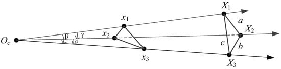
Figure 1.
The P3P problem.
In Figure 1, let OC be the center of perspective, be the 3D control points and be their image projections. The 3D points are known in the world frame and let , , . In the existing P3P solvers, the camera is fully calibrated and then , , can be computed as with the camera intrinsic parameters (focal length, principal point) and image projections . We assume , , and from triangles , , , we obtain the P3P equation system:
The P3P problem is to obtain a set of solutions for , , and this problem is known to provide up to four possible solutions that can then be disambiguated using a fourth point.
2.3. Problem Statement and Method
2.3.1. Problem Statement
The strict requirement of full calibration for the camera in the P3P solvers prevents its application from these cases where some intrinsic parameters might change online or be unknown. In this paper, these intrinsic parameters are the focal length, principal point and the problem is to solve the intrinsic and extrinsic parameter estimation by solving the P3P problem with a known camera position.
When the focal length and principal point are unknown, the cannot be computed in the P3P problem. Some algorithms are proposed for extrinsic parameter and focal length estimation by four 3D points [21] or for extrinsic parameter, focal length and principal point estimation by five 3D points [25]. However, user convenience dictates the use of as few 3D points as possible—accurate 3D points are troublesome and expensive to acquire and maintain. In some cases where the camera is fixed, the camera position can be obtained as prior knowledge and then our problem is to solve intrinsic and extrinsic parameter estimation with fewer 3D points and the known camera position. The problem is illustrated in Figure 2—let OC be the center of perspective which is known, be the 3D reference points, be their image projections and the task is to solve intrinsic (the focal length, principal point) and extrinsic parameter estimation from these information.
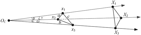
Figure 2.
Our problem.
In Figure 2, are computed by three 3D points and the camera position OC, not by camera intrinsic parameters (focal length, principal point) and image projections as in the traditional P3P problem as shown in Figure 1. Now our problem is summarized geometrically as follows—the image points are in the original image frame and let , , ; we assume , , and from triangles , , , we obtain the equations:
Now the task is to find a set of solutions for which is known to provide up to four possible solutions. This is similar to the P3P problem, but the variables and invariants of the equations have completely different meanings—a, b, c are the distances between every two image points, but they are the distances between every two 3D points in the P3P problem; is the distance between camera position OC and image point , but is the distance between the camera position OC and 3D point ; in addition, the way to obtain the values of is different, as described above.
In the following, our main work is to convert our problem to a P3P problem and obtain the values of intermediate variables which are then used for intrinsic and extrinsic parameter estimation and to lastly find the unique solution by image resolution. We provide our method of the problem as follows.
2.3.2. Proposed Method
In this section we convert our problem to a P3P problem as shown in Figure 3 and then obtain the values of intermediate variables by P3P solvers [13,16].
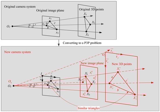
Figure 3.
Converting to a P3P problem.
From Figure 3, We systematically formulate this problem in the following basic procedures:
(1) This step involves the definition of three new 3D points and a new world frame from the original image points . is on the ray and , where d is pixel size. The new world frame is defined as , where
are parallel with the x-axis and y-axis of the original image frame, respectively. is on the ray and . Then, we can obtain the new 3D points in the new world frame:
(2) We make the original 3D points as the new image points . In addition, this step involves the definition of a new principal point and a new camera frame from the original 3D points . The new camera frame is defined as , where is the camera position OC and
Via the transformation matrix , the original 3D points in the original world frame SW can be transformed into using
Now we define a new camera system whose camera frame is and image plane S contains points . Then, the new principal point is the projection from the point to the plane S.
(3) The focal length of the new camera system can be given by .
(4) In a new camera system, the pixel size is 1 and the new image points can be obtained by
(5) Now we have obtained three new 2D-3D point correspondences and up to four possible solutions can be obtained by the existing P3P solvers. Via the solutions , points in new world frame can be transformed into using
Since the origin of the new camera frame is the camera position, the camera position in the new camera frame is . From the transformation between frame and , we obtain , and then the camera position of the new camera system in frame can be given by
Intrinsic parameter estimation. From the definition of the new world frame and the original image plane, we can obtain the relationship between the principal point, focal length of original camera system and camera position of the new camera system in frame as shown in Figure 4.
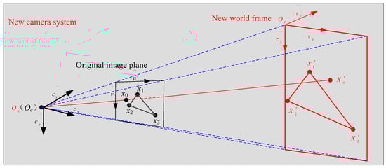
Figure 4.
New camera system.
In Figure 4, we assume is the projection from point to the plane S2 who contains points and as described above. is the intersection of the line and the original image plane. Because the plane S2 is parallel with the original image plane, is perpendicular to the original image plane. Point of the original camera system and point of the new camera system are the same point, therefore is perpendicular to the original image plane which means is the principal point and is the focal length of the original camera system. Now the principal point and focal length can be
Here, the values of the principal point and focal length are in pixel. However, there are up to four values of the principal point and focal length because of the four possible solutions of the P3P solvers.
(6) Determination of a unique solution. We assume the image resolution of the original camera system is which is known and then the ideal principal point can be given by
After giving the ideal principal point, the unique solution of principal point is obtained by
Note that has up to four points and the point closest to the ideal principal point is the unique principal point. When is the minimum, we let the unique solution be and focal length . Now the intrinsic parameter estimation is finished and finally the transformation between and is written as
(7) Extrinsic parameter estimation. From the definition of the original camera frame SC and the new world frame as shown in Figure 4, can be transformed into SC using
Here
In the following, we will focus on the transformation between SC and SW. Our method involves four frames , and the transformations between , , have been obtained, as shown in Figure 5.
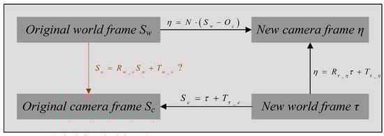
Figure 5.
Transformations of the four frames. The question mark there means the transformation between SC and SW is unknown and needs to be computed. This is different from the other transformations, which have been computed.
From these transformations, the original world frame SW can finally be transformed into the original camera frame SC using
Extrinsic parameter estimation is finally finished.
3. Experiments and Results
The method proposed in Section 2 will be thoroughly tested by synthetic data, and compared to Kneip’s [13] method and GP4Pf [21]. Kneip’s method returns up to four possible solutions and the disambiguation of the four possible solutions will be done using a fourth point.
Lastly, we test the proposed method with real images to verify the feasibility for intrinsic and extrinsic parameter estimation in practical application.
3.1. Synthetic Data
We synthesize a virtual perspective camera with zero-distortion, zero-skew and unit aspect ratio. The principal point lies at the image center. The image resolution is 1280 × 800 pixels and the focal length is 50 mm. The position of the camera is fixed at , and the orientation is kept at , which means the camera frame SC and world frame SW are parallel.
The synthetic data consist of three thousand 3D points that are randomly generated in the world frame. These points are randomly distributed in the box of [−20, 20] × [−2, 2] × [190, 210]. For each test, three synthetic 3D points are randomly selected from the synthetic data, and project them into image points using the virtual perspective camera. Now the synthetic data have three thousand 2D–3D point correspondences.
3.1.1. Numerical Stability
To analyse the numerical stability of our proposed method, we perform 50,000 trails. At each trail, we randomly select three 2D–3D point correspondences from synthetic data without any noise added to the 2D image points for our proposed method and Kneip’s method, and four 2D–3D point correspondences for GP4Pf. We measure the log10 value of the relative error between the ground truth and the estimated focal length by our proposed method and GP4Pf. The results are shown in Figure 6a. We measure the log10 value of the error in translation by our proposed method, Kneip’s method and GP4Pf, as shown in Figure 6b.
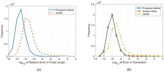
Figure 6.
(a) Relative error in focal length. (b) Error in translation.
From Figure 6a, the distribution of the log10 value of the relative error between the estimated focal length and the ground truth can be observed. We can see our proposed method is clearly superior in numerical stability over GP4Pf which is the state-of-the-art 4-point solution.
From Figure 6b, the distribution of log10 value of error in translation can be observed. We can see our proposed method is clearly superior in numerical stability over GP4Pf and compared to Kneip’s method, it behaves in a very similar way, but Kneip’s method has a multi-solution phenomenon that is up to four solutions and needs a fully calibrated camera.
3.1.2. Noise Sensitivity
In this Section, we add zero-mean Gaussian noise onto the image points. We vary the noise deviation level δ from 0 to 2 pixels. At each noise level, we run 50,000 independent trails and report the median focal length, translation, rotation, and reprojection error in Figure 7.
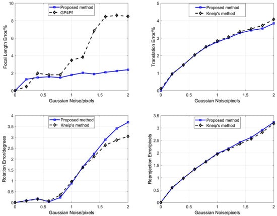
Figure 7.
Experiment results of noise sensitivity.
Based on Figure 7, in terms of the relative focal length error, our proposed method is better than GP4Pf. In terms of the relative translation and reprojection error, our proposed method and Kneip’s method have similar performance. In terms of the rotation error, our proposed method is slightly worse than Kneip’s method, but Kneip’s method has a multi-solution phenomenon that is up to four solutions and needs a fully calibrated camera.
3.1.3. Computational Time
In this section, we perform 50,000 independent trails to analyze the computational time of our proposed method, the GP4Pf and the Kneip’s method executed on a 3.3 GHz 4-core laptop. At each trail, we randomly select three 2D–3D point correspondences from synthetic data without any noise added to the 2D image points for our proposed method and Kneip’s method, and four 2D–3D point correspondences for the GP4Pf. We report the average computational time in milliseconds (ms) in Table 1.

Table 1.
Computational time.
From Table 1, we observe that our proposed method is faster than the GP4Pf and is slightly slower than Kneip’s method, but Kneip’s method has a multi-solution phenomenon that is up to four solutions and needs a fully calibrated camera.
3.2. Real Images
We have also tested our proposed method using real images captured by two cameras with 1280 × 800 resolution. These cameras are assumed to have zero-distortion, zero-skew and unit aspect ratio. We place some control points in these two camera fields of view as shown in Figure 8.
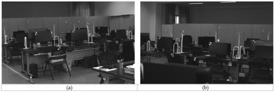
Figure 8.
(a) Left camera. (b) Right camera.
Because the ground truth of the intrinsic and extrinsic camera parameters in real scenarios is unknown, we cannot directly compare measuring precision of the intrinsic and extrinsic parameter estimation from real images. Therefore, we compare the precision of our proposed method, Kneip’s method and the GP4Pf indirectly—some control points are placed in the two camera fields of view, and the positions of these points and cameras are measured as the ground truth by a total station (NTS-330R, measuring precision is better than 0.5 cm). We use 3 or 4 control points for the intrinsic and extrinsic parameter estimation and the positions of the other points are measured by binocular vision. Then, the average error of relative position between the measured value and the ground truth is used to verify the accuracy of the intrinsic and extrinsic parameter estimation. The measuring result of relative position error is 0.43% with our proposed method, 0.47% with Kneip’s method and 1.37% with the GP4Pf. This shows our proposed method works well in real scenarios.
In addition, because the intrinsic and extrinsic parameter estimation only needs feature point extraction from real images, synthetic data and real images of simple scenes can be used to perform a thorough comparison with other PnP methods [13,21,23,25].
4. Discussion
The PnP problem originates from intrinsic and extrinsic parameter estimation and the PnP solvers are widely used in SLAM, computer vision and photogrammetry. In this paper, we propose a novel method for intrinsic and extrinsic parameter estimation. This method just needs three 3D points and the position of the camera, which is different from the existing PnP solvers. The differences and advantages of our proposed method are as follows.
4.1. Difference and Advantage
The P3P is the minimal subset of PnP and in some cases, it is difficult to acquire 3D points. This is the reason why we do our work with the P3P problem. However, P3P solvers needed a fully calibrated camera in previous studies, so we had the idea about extrinsic parameter estimation with an uncalibrated camera and three 3D points. From Figure 1, although , , cannot be computed with an uncalibrated camera in the original camera frame, they can be computed in the original world frame when the camera position is known. This finding let us convert our problem to the known P3P problem as shown in Figure 3. The thought is to build a new camera system whose camera frame is defined with the original world frame and the world frame is defined with the original camera frame. This is a P3P problem between the new camera frame and the new world frame. With the definition of a new camera system, three new 2D-3D point correspondences are obtained and then the extrinsic parameters of the new camera are obtained by the P3P solvers. There is an interesting point in this solution—the camera position in the new world frame contains the intrinsic parameter information of the original camera system, as shown in Figure 4. This is the key for intrinsic parameter estimation in our proposed method.
Additionally, the way to solve the multi-solution problem is different. The existing P3P solvers use a fourth point to disambiguate multi-solution phenomena, but our proposed method uses no extra point. The multi-solution phenomenon of P3P solvers in the new camera system leads to the multi-solution of the intrinsic parameter in the original camera system and hence we can obtain up to four principal points. This is because the image resolution is known and the ideal principal point can be obtained with Equation (14). The ideal principal point, not a fourth 3D point, can be used to disambiguate multi-solution phenomenon in our proposed method. In this paper, we assume the one closest to the ideal principal point is the unique principal point and this assumption yields good results with synthetic data and real images, as shown in Section 3.
In the new camera system, the new 2D image points are obtained from original 3D points which have the characteristics of high precision because they are measured by total station or other high precision measurement equipment. Therefore, the error of the new 2D point can be an order of magnitude lower than the error of the original 2D point and we think this may be a reason why our proposed method has improved numerical stability and lower noise sensitivity. Compared to the P3P method, only the establishment of the new frames and coordinate transformation are added in our proposed method, which can be made very fast, and this is the reason why our proposed method is just slightly slower than Kneip’s method. Our proposed method just uses three 3D points and this is a reason why it is faster than the GP4Pf that uses four 3D points.
In brief, we can see that the proposed method has the following advantages—(1) it just uses three 3D points and the camera position to estimate intrinsic and extrinsic parameters; (2) it has no multi-solution phenomenon; and (3) it has improved numerical stability and lower noise sensitivity.
4.2. Future Work
Our proposed method needs to know the camera position and uses the manual zoom lens in experiments, which means we cannot change the focal length constantly. Therefore, in the future, we will focus on real-time intrinsic and extrinsic parameter estimation for an auto-zoom camera. Additionally, our proposed method in Section 2 is suitable for a camera with fixed position. In the future, we will install a positioning device (e.g., RTK) on the camera and this means we can use a camera whose position is constantly changing. The work will expand the use range of our proposed method.
Another work that will be done in the future is to explain theoretically and experimentally why our proposed method has improved numerical stability and lower noise sensitivity.
5. Conclusions
We have proposed a novel method for intrinsic and extrinsic parameter estimation by solving a perspective-three-point problem with known camera position. By building a new camera system and converting our problem to the P3P problem, the unique solution can be obtained. Our proposed method just uses three 3D points, and has improved numerical stability and lower noise sensitivity. Experiment results show our proposed method works well in synthetic data and real scenarios. It is particularly suitable for estimating the focal length, principal point and pose of a zooming, uncalibrated camera with fixed position.
Author Contributions
Conceptualization, H.Y. and K.G.; methodology, K.G.; software, K.G. and J.G.; validation, H.Y. and K.G.; formal analysis, K.G. and J.G.; investigation, H.C.; resources, K.G.; data curation, J.G.; writing—original draft preparation, H.Y.; writing—review and editing, K.G.; visualization, J.G. and K.G.; supervision, H.Y.; project administration, H.C.; funding acquisition, H.Y. All authors have read and agreed to the published version of the manuscript.
Funding
This research received no external funding.
Institutional Review Board Statement
Not applicable.
Informed Consent Statement
Not applicable.
Data Availability Statement
The data presented in this study are available in the manuscript.
Conflicts of Interest
The authors declare no conflict of interest.
References
- Lu, X.X. A Review of Solutions for Perspective-n-Point Problem in Camera Pose Estimation. J. Phys. Conf. Ser. 2018, 1087, 052009. [Google Scholar] [CrossRef]
- Nakano, G. A versatile approach for solving PnP, PnPf, and PnPfr problems. In Proceedings of the European Conference on Computer Vision, Amsterdam, The Netherlands, 8–16 October 2016; pp. 338–352. [Google Scholar]
- Zhou, L.; Kaess, M. An efficient and accurate algorithm for the perspective-n-point problem. In Proceedings of the International Conference on Intelligent Robots and Systems, Macau, China, 3–8 November 2019; pp. 6245–6252. [Google Scholar]
- Zheng, Y.; Kuang, Y.; Sugimoto, S.; Astrom, K.; Okutomi, M. Revisiting the pnp problem: A fast, general and optimal solution. In Proceedings of the IEEE International Conference on Computer Vision, Sydney, Australia, 1–8 December 2013; pp. 2344–2351. [Google Scholar]
- Ferraz, L.; Binefa, X.; Moreno-Noguer, F. Very fast solution to the PnP problem with algebraic outlier rejection. In Proceedings of the IEEE Conference on Computer Vision and Pattern Recognition, Columbus, OH, USA, 23–28 June 2014; pp. 501–508. [Google Scholar]
- Lourakis, M.; Terzakis, G. A globally optimal method for the PnP problem with MRP rotation parameterization. In Proceedings of the International Conference on Pattern Recognition, Milan, Italy, 10–15 January 2021; pp. 3058–3063. [Google Scholar]
- Yu, Q.; Xu, G.; Zhang, L.; Shi, J. A consistently fast and accurate algorithm for estimating camera pose from point correspondences. Measurement 2021, 172, 108914. [Google Scholar] [CrossRef]
- Hartley, R.; Zisserman, A. Multiple View Geometry in Computer Vision, 2nd ed.; Cambridge University Press: Cambridge, UK, 2003. [Google Scholar]
- Wu, Y.; Tang, F.; Li, H. Image-based camera localization: An overview. Vis. Comput. Ind. Biomed. Art 2018, 1, 1–13. [Google Scholar] [CrossRef] [PubMed] [Green Version]
- Yuan, J.S.C. A general photogrammetric method for determining object position and orientation. IEEE Trans. Robot. Autom. 1989, 5, 129–142. [Google Scholar] [CrossRef]
- Wang, P.; Xu, G.; Wang, Z.; Cheng, Y. An efficient solution to the perspective-three-point pose problem. Comput. Vis. Image Underst. 2018, 166, 81–87. [Google Scholar] [CrossRef]
- Wolfe, W.; Mathis, D.; Sklair, C.; Magee, M. The perspective view of three points. IEEE Trans. Pattern Anal. Mach. Intell. 1991, 13, 66–73. [Google Scholar] [CrossRef]
- Kneip, L.; Scaramuzza, D.; Siegwart, R. A novel parametrization of the perspective-three-point problem for a direct computation of absolute camera position and orientation. In Proceedings of the IEEE Conference on Computer Vision and Pattern Recognition, Colorado Springs, CO, USA, 20–25 June 2011; pp. 2969–2976. [Google Scholar]
- Ke, T.; Roumeliotis, S.I. An efficient algebraic solution to the perspective-three-point problem. In Proceedings of the IEEE Conference on Computer Vision and Pattern Recognition, Honolulu, HI, USA, 21–26 July 2017; pp. 7225–7233. [Google Scholar]
- Masselli, A.; Zell, A. A new geometric approach for faster solving the perspective-three-point problem. In Proceedings of the International Conference on Pattern Recognition, Stockholm, Sweden, 24–28 August 2014; pp. 2119–2124. [Google Scholar]
- Gao, X.-S.; Hou, X.-R.; Tang, J.; Cheng, H.-F. Complete solution classification for the perspective-three-point problem. IEEE Trans. Pattern Anal. Mach. Intell. 2003, 25, 930–943. [Google Scholar]
- Grunert, J.A. Das pothenotische problem in erweiterter gestalt nebst über seine anwendungen in der geodäsie. Grunerts Archiv für Mathematik und Physik. 1841, Band 1, 238–248. [Google Scholar]
- Fischler, M.A.; Bolles, R.C. Random Sample Consensus: A Paradigm for Model Fitting with Applications to Image Analysis and Automated Cartography. Read. Comput. Vis. 1987, 24, 726–740. [Google Scholar]
- Camposeco, F.; Cohen, A.; Pollefeys, M.; Sattler, T. Hybrid camera pose estimation. In Proceedings of the IEEE Conference on Computer Vision and Pattern Recognition, Salt Lake City, UT, USA, 18–22 June 2018; pp. 136–144. [Google Scholar]
- Taketomi, T.; Okada, K.; Yamamoto, G.; Miyazaki, J.; Kato, H. Camera pose estimation under dynamic intrinsic parameter change for augmented reality. Comput. Graph. 2014, 44, 11–19. [Google Scholar] [CrossRef] [Green Version]
- Zheng, Y.; Sugimoto, S.; Sato, I.; Okutomi, M. A general and simple method for camera pose and focal length determination. In Proceedings of the IEEE Conference on Computer Vision and Pattern Recognition, Columbus, OH, USA, 23–28 June 2014; pp. 430–437. [Google Scholar]
- Wu, C. P3.5p: Pose estimation with unknown focal length. In Proceedings of the IEEE Conference on Computer Vision and Pattern Recognition, Boston, MA, USA, 7–12 June 2015; pp. 2440–2448. [Google Scholar]
- Bujnak, M.; Kukelova, Z.; Pajdla, T. A general solution to the P4P problem for camera with unknown focal length. In Proceedings of the IEEE Conference on Computer Vision and Pattern Recognition, Anchorage, AL, USA, 23–28 June 2008; pp. 1–8. [Google Scholar]
- Kanaeva, E.; Gurevich, L.; Vakhitov, A. Camera Pose and Focal Length Estimation Using Regularized Distance Constraints. In Proceedings of the British Machine Vision Conference, Swansea, UK, 7–10 September 2015; pp. 162.1–162.12. [Google Scholar]
- Triggs, B. Camera pose and calibration from 4 or 5 known 3d points. In Proceedings of the Seventh IEEE International Conference on Computer Vision, Corfu, Greece, 20–25 September 1999; Volume 1, pp. 278–284. [Google Scholar]
- Abidi, M.A.; Chandra, T. A new efficient and direct solution for pose estimation using quadrangular targets: Algorithm and evaluation. IEEE Trans. Pattern Anal. Mach. Intell. 1995, 17, 534–538. [Google Scholar] [CrossRef] [Green Version]
- Bujnak, M.; Kukelova, Z.; Pajdla, T. New efficient solution to the absolute pose problem for camera with unknown focal length and radial distortion. In Proceedings of the Asian Conference on Computer Vision, Queenstown, New Zealand, 8–12 November 2010; pp. 11–24. [Google Scholar]
- Josephson, K.; Byrod, M. Pose estimation with radial distortion and unknown focal length. In Proceedings of the IEEE Conference on Computer Vision and Pattern Recognition, Miami Beach, FL, USA, 20–25 June 2009; pp. 2419–2426. [Google Scholar]
- Guo, Y. A Novel Solution to the P4P Problem for an Uncalibrated Camera. J. Math. Imaging Vis. 2013, 45, 186–198. [Google Scholar] [CrossRef]
- Wu, Y.; Hu, Z. PnP Problem Revisited. J. Math. Imaging Vis. 2005, 24, 131–141. [Google Scholar] [CrossRef]
- Tsai, R. A versatile camera calibration technique for high-accuracy 3D machine vision metrology using off-the-shelf TV cameras and lenses. IEEE J. Robot. Autom. 1987, 3, 323–344. [Google Scholar] [CrossRef] [Green Version]
Publisher’s Note: MDPI stays neutral with regard to jurisdictional claims in published maps and institutional affiliations. |
© 2021 by the authors. Licensee MDPI, Basel, Switzerland. This article is an open access article distributed under the terms and conditions of the Creative Commons Attribution (CC BY) license (https://creativecommons.org/licenses/by/4.0/).